Determinants of Losses on Construction Loans: Bad Loans, Bad Banks, or Bad Markets?

WORKING PAPER SERIES

Determinants of Losses on Construction Loans:

Bad Loans, Bad Banks, or Bad Markets?

Emily Johnston Ross

Federal Deposit Insurance Corporation

Joseph B. Nichols

Board of Governors of the Federal Reserve System

Lynn Shibut

Federal Deposit Insurance Corporation

August 2021

FDIC CFR WP 2021-07

fdic.gov/cfr

The Center for Financial Research (CFR) Working Paper Series allows CFR staff and their coauthors to circulate

preliminary research findings to stimulate discussion and critical comment. Views and opinions expressed in CFR Working

Papers reflect those of the authors and do not necessarily reflect those of the FDIC or the United States. Comments and

suggestions are welcome and should be directed to the authors. References should cite this research as a “FDIC CFR

Working Paper” and should note that findings and conclusions in working papers may be preliminary and subject to

revision.

Determinants of Losses on Construction Loans:

Bad Loans, Bad Banks, or Bad Markets?

Emily Johnston Ross

Federal Deposit Insurance Corporation

Joseph B. Nichols

Board of Governors of the Federal Reserve System

Lynn Shibut

Federal Deposit Insurance Corporation

August 2021

Abstract

Construction loan portfolios have experienced notoriously high loss rates during economic

downturns and are a key factor in many bank failures. Yet there has been little research on what

drives losses on construction loans and how to mitigate those losses, due to a lack of data. Using

proprietary loan-level data from more than 15,000 defaulted construction loans at over 275 banks

that failed between 2008 and 2013, we explore the extent to which observed losses during a

severe downturn are driven by the characteristics of the loans, the originating banks, and the

local markets. We find close ties between loss rates and certain loan characteristics as well as

market conditions both at and after origination, while institution-level differences across banks

appear less important. We find that the risk of higher losses on construction loans is influenced

not only by the originating bank’s behavior but also by the behavior of other local lenders in the

market. This finding has important implications for how lenders and regulators manage risk

through the real estate cycle. We also find support for existing regulatory guidance regarding

higher capital requirements for construction loans, specifically for land and lot development

loans.

JEL Classification Codes: R31, R33, G21

Keywords: ADC, Construction Loan, LGD, CRE.

The views and opinions expressed in this paper reflect the views of the authors and not

necessarily those of the FDIC, the Board of Governors of the Federal Reserve System, or the

United States. The authors wish to thank Lily Freedman, A.J. Michelli, and Michael Pessin for

research assistance; Suzi Gardner, Derek Johnson, Michael McCann, and Ken Redline for expert

advice; and Domenic Barbato, Rosalind Bennett, Mike Brennan, Kayla Freeman, Lisa Garcia,

Peter Martino, Ajay Palvia, Smith Williams, and Mary Zaki for useful comments. All errors and

omissions are our own.

550 17

St NW, Washington, DC 20429, [email protected]

and C St NW, Washington, DC 20551, joseph.b.nichols@frb.gov

550 17

St NW, Washington, DC 20429, [email protected]

1. Introduction

The construction sector of the economy is inherently cyclical. Figure 1 presents residential and

nonresidential construction investment in the United States from 1960 to 2020 and reveals a

series of large swings for both types of collateral. The bust was especially strong in the Great

Recession, with a peak-to-trough decline of 79 percent for residential investment and 51 percent

for nonresidential and multifamily investment.

An important contributor to this high degree of

cyclicality in the construction sector is the stickiness of construction spending, caused by the

time required to plan, finance, and construct a project. Many commercial projects take three or

more years to complete, making it difficult to quickly adjust the level of investment in response

to demand shocks.

Figure 1: Level of Investment in Construction from 1960 to 2020

It is not surprising, then, that construction loans have often played a significant role in

weakening bank balance sheets and contributing to bank failures during periods of financial

distress.

Noncurrent loan rates for acquisition, development, and construction (ADC) loans at

U.S. banks were more than double the noncurrent rates of other types of mortgages during both

Residential investment peak is 2005Q4 and trough is 2009Q2, while for nonresidential investment the peak is

2008Q2 and the trough is 2011Q1.

For example, see Grenadier (1995) and Wheaton (2014).

We include in our analysis not only loans for the construction of the actual buildings but also loans to acquire the

land itself and loans to develop the lots before the actual building construction (i.e., putting in curbs and pipes, etc.)

For the remainder of the paper, construction loans refer to the subset of loans that finance the construction of the

actual buildings.

the Great Recession and the 1980 to 1994 banking crisis.

Researchers have also found that

banks with heavy exposures to ADC loans were more likely to fail during both crises.

broadly, periods of real estate speculation have frequently contributed to financial crises around

the world.

Thus bankers need to approach ADC loans with appropriate caution and expertise,

and banking regulators need to set policies and procedures that suitably address the risk.

Unfortunately, there is much less information in the literature about what triggers losses for ADC

loans than for retail loans, corporate loans, or mortgages on existing residential and commercial

properties. Other types of loans often use nonbank financing, such as public debt markets or

securitization, that provide publicly available loan performance data for empirical studies.

ADC loans instead have, until recently, been limited to bank financing. As a result, data

availability has severely restricted research on ADC loan performance. In fact, we are unaware

of any empirical research that focuses on loss given default (LGD) for ADC loans, despite its

critical importance to the losses of this high-risk asset class.

This paper fills this hole in the literature by using a unique and proprietary set of loan-level data.

The goal of this paper is to learn about the factors that drive distressed LGD for ADC loans and

to explore the implications for lenders and regulators. We decompose LGD on ADC loans into

components that can inform bankers, investors, and regulators about risk exposures in actionable

ways. We then group the explanatory variables into loan, bank, and market characteristics, and

we examine the sensitivity of LGD to each group. Losses due to poor underwriting or poor bank

management can be mitigated through changes in lending policies and supervisory oversight.

Other factors that are not under direct control of the lender, such as losses tied to changes in

market conditions post-origination, are best addressed by loss reserves or capital requirements.

We analyze LGD for a sample of more than 15,000 loans from over 275 failed banks that were

resolved by the FDIC from 2008 to 2013. Most of these loans were originated during the boom

period in the mid-2000s, defaulted during the Great Recession, and were worked out during and

after the Great Recession. We acknowledge that this sample is hardly random: clearly we are

oversampling bad loans at bad banks during a very bad time.

However, we feel that this is

Author calculations using Call Report data. From 2008 through 2013, the noncurrent rate for ADC loans peaked at

16.8 percent, single-family peaked at 8.1 percent, and the others (C&I, multifamily, and other CRE) peaked below 5

percent. From 1991 to 1994, ADC loans peaked at 14.1, and the next highest loan type (other CRE) peaked at 5.5

percent. Data are not available for most loan types before 1991.

See GAO (2013) and Friend, Glenos, and Nichols (2013) for analysis of the Great Recession. See Fenn and Cole

(2008) and Collier, Forbush, and Nuxoll (2003) for analysis of the 1980 to 1994 crisis.

Both Kindleberger (2000) and Reinhart and Rogoff (2011) cite speculation in various forms of construction and

real estate as an underlying cause for many historical financial crises.

See, for example, Altman, Resti, and Sironi (2004) and Downs and Xu (2015).

We perform a benchmarking exercise in Appendix B, comparing our data against losses on construction loans

from a separate and independent supervisory data collection for large banks. We find differences between the two

samples, but we also find credible explanations for these difference that relate to the composition of the sample

precisely the sample one would want to work with to explore the drivers of ADC loan risk. It is

losses on bad loans during bad times that account for the majority of ADC losses at banks and

are the most damaging to the banking industry. And it is the drivers of distressed LGDs that is

what is interesting, as aggregate losses on construction loans during benign periods have

historically been negligible.

One of our key findings is that banks exert no direct control over some factors that heavily

influence distressed LGD. More specifically, we find two factors related to local markets at the

time of default: the share of noncurrent ADC loans held by local lenders when the loan defaults,

and the change in the local ratio of ADC loans to total loans between origination and default.

Higher local noncurrent rates for ADC loans at the time of default are an indication of markets

that are experiencing distress. At the same time, an increase in local ADC lending between

origination and default shows the extent to which other lenders are leaning into the market. If a

local area has both strongly increasing ADC lending and relatively high local noncurrent rates at

the same time, the local market may be unstable or overheating. We would expect to observe

higher losses on loans defaulting in these markets. We believe that the sensitivity of losses for

ADC loans to changes in these local market factors post-origination provides a strong argument

supporting the use of higher capital requirements and lower loan-to-value (LTV) limits than for

less cyclically sensitive loans.

We document the importance of market conditions at loan origination as well. The bank’s

decisions regarding when and where to make ADC loans are not exogenous: they reflect a bank’s

ability to properly assess and manage risk based on information available when the lending

decision is made. We find that loans originated in markets with higher proportions of ADC loans

to total loans are associated with higher losses, and loans originated in markets with higher ADC

lending growth in the period leading up to origination also have higher losses. Local markets

with outsized ADC lending exposure and faster ADC loan growth at origination may contribute

to higher losses through multiple channels, such as less experienced lending officers and

builders, weaker loan covenants, and less focus on risk exposures. In highly competitive markets,

lenders are well aware that they can originate loans only if their loan terms and covenants are

competitive. They may pay insufficient attention to increases in the supply of homes and

buildings (including the extent of new inventory that will or may soon arrive), optimistic

construction budgets or real estate appraisals, or environmental or other construction risks. Given

the time delay required to complete construction and the inability to adjust investment quickly, a

risk of oversupply under such conditions may be heightened.

(such as size and geography) and variable definitions, increasing our confidence in the representativeness of the

FDIC loan data.

The noncurrent rate for ADC loans, as reported in the Call Report, soared from 0.8 percent as of year-end 2006 to

16.8 percent as of March 31, 2010. The peak rate for ADC loans was more than double the peak rate for other loan

types.

We find that loan characteristics also explain a large share of the variation in LGD. Loans for

projects earlier in the development cycle, specifically those to purchase land and develop lots,

had significantly higher losses than loans for the actual construction of either single-family or

commercial buildings (“vertical” construction). This supports tighter capital and LTV guidance

for these loans. We find that smaller loans in our sample also have higher loss rates. The location

of the project matters, with loans outside of the originating bank’s footprint or in a judicial

foreclosure state

having higher losses as well. We do not observe a significant difference in

LGD between single-family and commercial construction loans.

We examine several loan-level characteristics based on the observed performance of the

mortgages post-origination. This includes the timing of the default (specifically the age of the

loan at default) and whether the loan defaulted at the expected maturity of the loan (a “maturity

default”). We also include the share of the committed balance that has been drawn at the time of

default and whether the bank allowed the borrower to draw more than what was originally

committed (an “overage”). These loan-level variables at default reflect a combination of

borrower/builder performance and the monitoring function of the lender. From a collateral

perspective, these variables may reflect the extent of progress made in creating collateral value

through construction.

In contrast to market and loan characteristics, bank-level factors seem to explain much less of the

variation in LGD. These include broad measures that are readily comparable across banks, such

as asset size or portfolio growth, which may, for example, reflect institutional differences in

specialization or in how loans are originated or monitored. We find that larger banks tend to

suffer lower losses in default. We also observe that LGD is higher when the bank had high ADC

loan growth leading up to origination and when it spent a longer time in distress before failure.

But overall, the impact of bank-level characteristics on LGD appears much smaller than loan-

level or market-level characteristics.

Our results have important implications to both bankers and regulators. When the demand (or

speculative demand) for new homes and buildings triggers a sustained strong increase in ADC

lending, the conditions for overbuilding—followed by high ADC defaults and high LGD on

defaulted loans—strengthen. Banks would be well served by astute credit risk functions that are

well informed about the risks that ADC loans pose during periods of distress, and how those

risks are exacerbated when the local market experiences a sustained period of new construction

and high levels of competition. While good underwriting and loan monitoring processes within

the originating bank will mitigate losses during periods of distress, the actions of other local

lenders and builders may contribute to oversupply in the market. Bank examiners should look for

evidence that banks understand these risks, have the appropriate levels of loss reserves, actively

That is, a state where a court order is required for foreclosures.

monitor for potential overbuilding, and do—or stand ready to—pull back their lending or

promptly take other actions to reduce their exposures as risks increase.

The rest of the paper is organized as follows. Because lending related to construction has unique

traits that influence LGD, Section 2 provides institutional background information that informs

our analysis. Section 3 discusses the FDIC Loss Share Administration program and the data used

for our analysis. Section 4 lays out the methodology, Section 5 provides the results, and Section

6 discusses the implications of those results. Section 7 concludes.

2. Institutional Background

Several unique aspects of ADC loans set them apart from other mortgages. The most significant

difference from the perspective of modeling losses is that a large share of the collateral that

backs ADC loans is created during the loan term. There is no cash flow from rents available to

service the debt. There is no rental history upon which to base a valuation, merely a speculative

estimate of value based on market conditions as of the expected completion date. This is a

foundational difference that influences the loan origination and servicing processes, the loan

terms, and the lender’s risk exposure. Section 2.1 begins by explaining the processes involved in

originating and managing these loans and the loan terms. Section 2.2 discusses the lender’s risks

from ADC loans and how they relate to the nature of the collateral, the loan administration

processes, and the loan terms. In both sections, ADC loans are compared with other, more

familiar, types of real estate loans,

and relevant academic literature is discussed.

2.1 Loan Processes and Terms

This section begins with a discussion of the typical loan origination process and loan terms,

followed by sections on the collateral valuation at origination, the monitoring process, default,

and the loan workout process.

2.1.1 Loan Origination and Loan Terms

Investors frequently form a Limited Liability Corporation (LLC) for each specific project. The

LLC acts as the official borrower, who hires a builder to do the construction; sometimes the

builder is the investor. The investor normally purchases the property and places it in the LLC (if

any), designs the construction project, hires the builders, and completes the entitlement process

before origination.

The term to maturity for ADC loans is relatively short, and larger projects usually involve

multiple loans. For example, for a single-family housing development, the borrower might obtain

a land development loan to put in curbs, underground pipes, and electrical service and a separate

Specifically, to a typical first lien for a single-family home or commercial real estate loan (CRE) loan.

This section is based on anecdotal information from discussions with bankers, examiners, and other experts.

That is, the process of obtaining the zoning changes and other regulatory approvals that are required before

construction begins.

construction loan to build the houses. Even single construction loans are often structured in

tranches, with the next segment of the committed balance being issued to the borrower only if

certain thresholds are met. For larger office/retail complexes, there may be separate loans or loan

tranches for each phase of development. Many ADC loans include a “permanent” (that is, long-

term) financing phase once construction is complete and other thresholds are met.

A large

share of the profits come from fees at origination. The loan structures for other types of

mortgages are more permanent and less complex, with interest income comprising a larger share

of the lender’s profit.

ADC projects rarely produce income for the borrower until construction is complete and the

property is either leased to tenants or sold. Therefore, the loans are normally structured with an

interest reserve with no payments due directly from the borrower until maturity (or, in the case of

single-family developments, as homes are sold). With an interest reserve, the total amount of the

loan includes funds disbursed to the borrower and undisbursed funds that are used to cover

interest expenses during the loan term. This structure contrasts with other types of mortgages,

where regular payments are due throughout the loan term (and which serve as a key measure in

determining default).

The payment stream to the borrower also differs markedly from other mortgages. For single-

family residential (SFR) and commercial real estate (CRE) mortgages, the full loan amount is

normally disbursed at origination. For ADC loans, the loan documents set forth a pre-defined

schedule, where new disbursements are made as various phases of construction (or in some cases

sales or leases) are completed. The requirements for each tranche of the loan to be disbursed are

spelled out in the loan covenants. Disbursements are often relatively modest during the early part

of the loan term.

One other significant difference between ADC loans and other mortgages is the prevalence of

recourse. Lenders frequently require borrowers to provide personal guarantees to back ADC

loans. These guarantees, or recourse, provide some “skin-in-the-game” on the part of the

borrower, if the value of the raw land or partially built project that is pledged as collateral is not

sufficient. Recourse is less frequently used for other types of mortgages, where the equity share

of the existing property pledged as collateral provides the “skin-in-the-game.” Glancy, et al.

(2021) find that recourse in transitional loans (defined as construction and redevelopment loans)

is correlated with unobserved risks, as transitional loans with recourse have higher spreads at

origination and worse performance during the COVID pandemic, however they are looking at

the impact of recourse on default and not recovery rates.

For example, for a multifamily loan, a specified share of the apartments might have to be leased.

2.1.2 Valuation at Origination

Banks must decide whether to originate an ADC loan based on the potential value of the project,

which is by definition unobserved. Third-party certified appraisers are hired during the loan

approval process and must adhere to well-developed standards that govern estimation methods

and the products they produce.

Loan commitments often occur before the appraisal is

complete—and are often conditional on the appraised value—but loan originations always occur

after the appraisal. Appraisals for construction projects are by their nature more speculative than

for existing buildings, where historical rental cash flows are available.

Banks normally request both an “as is” appraised value and one or more “as will be” appraised

value(s). There are two standard “as will be” measures of value. The first, known as “as

stabilized” value, represents the value for the finished project when the appraiser assumes that

the property is already built and leases have stabilized or finished lots or homes have been sold

as of the appraisal date. The second, known as the bulk value, represents a value based on a

discounted cash flow approach when the appraiser develops assumptions about the time needed

for building, the time needed for lease stabilization or asset sale(s), the future value of the

finished project, and then discounted the estimated future value to the appraisal date. Finished

product values are invariably higher, and banks used them more often—and relied on them more

heavily—during boom periods. We expect that, especially when markets are shifting, the

appraisals are significantly less reliable for construction projects than for other real estate.

2.1.3 Loan Monitoring

The monitoring process for ADC loans is much more labor intensive than for other mortgages

and often requires detailed knowledge of construction, the local regulatory approval process, the

loan contract details, the local market, and the title insurance process. Over the term of the loan,

the lender monitors the progress of the construction, including items such as the receipt of

materials, payments to suppliers, progress on the building(s), and associated regulatory

approvals. Based on the status of the construction and the loan covenants, the lender determines

when draws can be made, the size of the allowed draws, whether and how the loan terms should

be adjusted (if construction problems arise or markets shift), and when payments are due.

Adjustments are commonplace as the construction progresses and may arise because of issues

such as changing prices for labor or materials, delays in receiving materials, subcontractor

availability, environmental problems, poor quality construction, or changes in local demand.

2.1.4 Loan Default

The timing of loan default falls into two categories: term defaults and maturity defaults. Maturity

defaults occur when the borrower is unable to sell the collateral at an adequate price, or, for

commercial properties, when the borrower cannot obtain sufficient permanent financing to pay

See Appraisal Standards Board (2017) for details.

off the ADC loan in full.

Because the borrower does not make regular payments, term

defaults

are almost always determined by the lender (or in some cases bank examiners); they

are frequently based on an evaluation of the local market conditions and anticipated demand, or

on the borrower being unable to meet performance covenants. This contrasts sharply with other

types of mortgages, where borrowers make regular payments and default is simply determined

by payment delinquency.

Because loan default involves judgment on the part of the bank, the

timing may be less consistent across banks for ADC loans.

2.1.5 Loan Workout

The workout process for ADC loans is more complex and the lender’s negotiating position is

weaker than in the other types of mortgages, for two reasons. First, the investor’s equity position

is more likely to be deeply negative, especially during a severe crisis.

Thus investors may be

unwilling or unable to bring additional capital to the project or monitor the building process.

Second, and more importantly, the builder has considerable scope to influence the outcome and

incentives that rarely align with those of the lender. The construction industry is highly cyclical,

and during distress periods builders are retrenching and desperate for cash to pay staff and fund

operations. With no new construction projects available, builders aggressively seek additional

draws from existing loans to survive. They rarely have any reason to cut back on existing

projects, regardless of whether demand exists for the finished project. All the loan participants

are well aware of the high cost of changing builders in the middle of a project and the significant

discount to market value for an incomplete building, and builders and investors can use that

knowledge at the lender’s expense during negotiations.

2.2 Risks

We now link some of the institutional aspects of ADC lending to specific risks that can help

drive losses. We divide these risks into four separate, but often interrelated, topics: construction

risks, the opacity of ADC loans, the option value of land, and sensitivity to real estate cycles.

Both construction risks and opacity contribute to the higher level of idiosyncratic risk of

construction loans, while the option value of land and the sensitivity to real estate cycles

contribute to the higher level of cyclical risks for ADC loans. We provide a summary of risks in

Appendix A.

In some cases, this takes the form of being unable to meet the lender’s requirements for a conversion to permanent

financing (that is a conversion to a CRE loan).

Term defaults occur before the maturity of the loan. We define maturity defaults as defaults that occur within 90

days of maturity or after maturity. All other defaults are term defaults.

In some cases, lenders may place CRE loans into nonaccrual status even when payments are current, because the

value of the collateral has dropped and the lender no longer expects full repayment of the loan at maturity. This is

common in the commercial mortgage-backed securities (CMBS) market, where the master servicer will transfer

such a loan to the special servicer to begin the loan workout process even if the loan is still current.

However, banks have some scope to restructure other types of troubled loans in ways that minimize reported

defaults, known as “evergreening.” This type of restructuring is less likely to occur for single-family mortgages

because most of them have standard terms.

In some cases, solvency may be uncertain or positive but the investor is illiquid.

2.2.1 Construction Risks

Cost overruns for construction projects are commonplace. Problems often begin with the budget

itself, which may suffer from optimism bias, inadequate feasibility analysis, omissions of

required items, or simplistic assumptions that do not adequately consider risks or entrepreneurial

profit. Other problems can include bad weather; delays in the availability of subcontractors, staff,

materials, or government inspectors; design changes and scope creep; cost increases for labor or

materials; unexpected underground conditions and other environmental problems; inexperienced

builders; or foul play and corruption.

The potential for these challenges to arise results in the

need for ongoing, and costly, monitoring of ADC loans by the lender.

2.2.2 Opacity

As discussed in Section 2.1, the lending function for ADC loans involves more complicated

terms and conditions than for other types of mortgages. The loan monitoring process is more

complex, and determining whether the loan is in default is more ambiguous. The loan workout

process is more likely to depend on stakeholders with incentives that differ markedly from the

lender. Loan guarantees are used more frequently, and the value of these guarantees are not

readily discernable. The appraisal process requires more estimation that introduces more

opportunities for error, and the construction process involves numerous potential pitfalls that are

not immediately obvious. Taken as a whole, these characteristics support a conclusion that ADC

loans are more opaque than other mortgage types. This opacity explains why there is no

standardized underwriting process and why banks usually retain ADC loans in their portfolios. It

also may magnify the scope for lender myopia or overconfidence.

2.2.3 Option Value of Land

A wide range of research exists on the option value of land, from Quigg (1993) to Munneke and

Womack (2020). The underlying theory is that all land, both developed and undeveloped, is

valued based on its highest and best use. Geltner et al. (2014) documented how the highest and

best use may change over time in response to changes in the local market and demand for space.

Property whose highest and best use was as a farm may instead now have a highest and best use

as single-family residences. Once the option value of developing the land (or redeveloping it to

change the property type) reaches a certain threshold, the project becomes viable and can acquire

investment and financing.

One aspect of the option value of land that is relevant to thinking about potential loss on

construction loans is the limited reversibility of investment. When the project starts, the highest

and best use might be single-family residential. However, once the project reaches completion,

the highest and best use may have shifted due to market developments and is now retail. The

See Ahiaga-Dagbui and Smith (2014) for additional discussion.

physical aspects of the project are difficult to reverse: for example, the street plan for a housing

development would not serve an office park.

But zoning restrictions can often be even more difficult to reverse. Before loan origination,

builders must obtain local approvals to construct the building(s) and, for single-family

developments, break the property into separate lots for future sale, which is often time-

consuming and politically challenging. This process can add substantial value to the project: on a

per-acre basis, the value of timberland or farmland is often a fraction of the value of the same

acreage (in the same condition and location) that has been approved for homes or a retail

shopping center. But it also represents a stickiness in terms of optimal land use. For example, if

agricultural land had been re-zoned as residential, it could be costly—or politically impossible—

to transition it to another higher best use. The option value of the land is “spent” once the project

has begun. A shift in demand during a project’s lifetime could lead to higher losses on the ADC

loan.

2.2.4 Sensitivity to Real Estate Cycles

LGD for ADC loans is far more sensitive to real estate price changes than other types of

mortgages, for several reasons. First, substantial time elapses between the date the lender

commits to the loan and completion of the construction. This lag is caused by the time to build,

which is often longer than the original estimate because of time lost to address supply problems

and subcontractor schedules, longer-than expected regulatory approvals (such as demolition,

environmental impact, various stages of construction, and sometimes zoning), and investor and

lender decisions associated with change requests, and lender inspections and approvals for

draws. Major market shifts can occur between the loan commitment date and the completion of

construction.

The potential for losses relating to the time delay between origination and

completion is compounded by two additional factors: (a) strong incentives for builders to

continue building during periods of distress regardless of the declining value of the finished

product, and (b) potential weaknesses in appraisals, such as reliance on “as stabilized”

valuations.

Second, most construction projects end with empty buildings, and the borrower’s ability to repay

the loan is generally contingent on finding buyers or tenants for the finished product.

Relocation costs, and the transaction costs for purchasing real estate, are substantial and may

hinder sales or leases. Relatively few ADC loans are backed by owner-occupied buildings or

projects with significant levels of pre-leasing or pre-sale contracts in place at the time of loan

commitment. During periods of serious distress, pre-leasing and pre-sale agreements can fall

See Grenadier (1995) and Wheaton (1999) for additional discussion. Both authors cite this time lapse as a

contributing factor to real estate cycles.

Or, for horizontal construction, approval of a new loan for the next phase of construction.

through. On the other hand, many commercial leases are long-term. These phenomena mitigate

losses for other types of residential and commercial mortgages but amplify the sensitivity to

business cycles for ADC loans.

Third, while all loan types are affected by heightened competition during boom periods, ADC

loans tend to be more strongly affected. ADC loan growth was much stronger than other loan

types during the boom before the Great Recession: from year-end 2003 to year-end 2007, ADC

loans held by banks increased 131 percent, but other types of mortgages held by banks increased

45 percent.

Lenders with a stronger appetite for growth—and thus a higher willingness to take

on risk—gravitated to ADC loans, most likely because it was easier for them to gain market

share.

For example, as of year-end 2007, the median ratio of ADC loans to total loans held by

de novo banks was 17 percent; the ratio was only 5 percent for banks that were ten years old or

older and had the strongest CAMELS composite rating.

During boom periods, lenders may feel

pressure to grow quickly, and the benefits of monitoring (including tight loan covenants)

diminish while the costs remain constant.

In addition, the average experience levels of lending

officers and builders declines. New builders are more likely to make mistakes, both in the cost

estimation process and the construction itself. New lending officers have less knowledge of and

skill in all aspects of the loan origination process, and they lack memories of the high costs

associated with real estate downturns. Lusht and Leidenberger (1979) found empirical evidence

that both builder and lending officer experience reduced the probability of default for

construction loans; there is good reason to expect the same for LGD.

3. Data

This section introduces the FDIC Loss Share Administration data that are the primary data used

in the paper. We then discuss the construction of our LGD measure, including a decomposition

of the loss into different components. The decomposition supports the comparison of our LGDs

with those from other sources that may contain different components. We then provide a range of

See Grenadier (1995) for additional discussion.

Percentages derived from bank Call Reports. See Rajan (1994) for additional discussion and evidence that

heightened competition results in looser bank lending policies (such as relaxed underwriting criteria and less

stringent monitoring).

According to bank Call Reports, as of year-end 2006 (at the height of the boom), de novo banks, banks with high

loan growth rates, and banks that relied heavily on brokered deposits all had higher concentrations of ADC loans

and higher ADC loan growth rates than other banks. Yom (2005) discusses the incentives for de novo banks to grow

quickly.

Data from bank Call Reports and examinations. De novo is defined as eight years old or younger. For the second

group, only banks with a CAMELS composite rating of 1 are included in the calculation. CAMELS ratings are

supervisory designations of bank condition and range from 1 (very strong) to 5 (very weak).

At least as long as the boom continues. See Rajan (1994) and Levitin and Wachter (2013) for evidence and

discussion on pressure for earnings and asset growth during boom times. See Ruckes (2004) for an analysis of the

net benefit of loan monitoring across the cycle.

There is substantial evidence of the same phenomenon for lending more generally. See, for example, Berger and

Udell (2003) and Rötheli (2012).

descriptive statistics about our loss data, both overall and across different regions and property

types.

We end with a brief discussion of potential concerns about our data.

3.1 FDIC Loss Share Administration Data

In this study, we use LGD data from banks that failed and were resolved by the FDIC in the

aftermath of the 2008 financial crisis. Loan portfolios held by failed banks oversample the upper

end of the credit loss distribution of ADC loans, and they should incur higher default rates than

portfolios at healthy banks. The nature of this sample selection works to our benefit. A signi-

ficant driver of losses to a bank will depend on the performance of the worst-performing loans in

their portfolio. A lending institution’s solvency is not dependent on the performance of the

median loan, but by the performance and losses in the upper tail of the credit loss distribution.

The FDIC has a loss share program to help dispose of assets from failed banks. From 2008

through 2013, the FDIC sold $39 billion in ADC loans from 289 failed banks to 144 bank

acquirers with loss share coverage. Most of the FDIC loss share agreements provided the

acquirers with 80 percent indemnification from credit losses for five years for assets covered

under the agreement (thus acquirers would absorb just 20 percent of the losses).

To manage its

risk exposure and support program administration, the FDIC collected information from the

failed banks as of the sale date (that is, the date the bank failed) and through detailed quarterly

reporting requirements from the acquiring banks after the sale date. Note that when we refer to

bank characteristics in this paper, we are referring to the characteristics of the failed bank that

originated the loan and not the acquiring bank that serviced the loan. The dataset contains data

from the inception of the program in 2008 through year-end 2015.

One of the unique aspects of the loss share program data is its detail on the components of the

losses. As we discuss further in Section 3.2, most existing LGD data in the literature do not have

this level of detail. Loss share LGD components include

• Charge-offs (net of recoveries);

• Loss on sale of asset (loan or other real estate owned (ORE));

• Expenses (legal fees, foreclosure expenses, appraisals, property maintenance costs, etc.)

paid to third parties related to the asset, except servicing fees; and

• Up to 90 days of accrued interest.

Given that the loan level data we use are by definition drawn from failed banks, Appendix B provides a

benchmarking exercise with a separate and independent set of data on defaulted construction loans from the Federal

Reserve’s FR Y-14Q Schedule H.2.

Compared with surviving banks, failed banks had higher ratios of ADC loan exposure to capital and higher loan

default rates during the Great Recession. This does not necessarily mean that they had higher LGDs. We tested

whether the individual bank’s loan default rate influenced LGD for our sample, and we found that the relationship

between LGD and the bank’s default rate was insignificant in most specifications.

For an additional three years, the acquirer was required to continue reporting all losses and recoveries, and to

continue to share recoveries (net of certain collection expenses) with the FDIC. However, most of the loss share

transactions were terminated shortly before or after the full indemnification period ended.

As of year-end 2015, either the loss share agreements had been terminated or the loss-sharing period had expired

for 243 of the 289 agreements. Only $860 million (2 percent) of the ADC loan portfolio was still active.

For loans foreclosed under the loss share program, the FDIC was entitled to share in any income

earned from the collateral. Losses from bulk loan sales were covered by the FDIC, but only if the

acquirer could demonstrate that a bulk loan sale was more cost-effective than loan-level (or

borrower-level) workout strategies. Therefore, bulk loan sales were rare.

The loans in our sample were originated by banks that failed. When the originating bank failed,

the loan underwent an ownership change during the loan term or workout period. This is not a

random sample of all defaulted ADC loans in the United States during the relevant time horizon.

To address concerns that our sample may not be representative of defaulted ADC loans at

privately held banks, we note that almost all of these loans were originated when the originating

banks were healthy and when there was substantial industry-wide growth in ADC loans. In

addition, Shibut and Singer (2015) compared LGD using similar data for commercial real estate

(CRE) loans backed by completed buildings from the FDIC’s loss share program to LGDs

reported in studies that relied on public sources (i.e., not failed banks). After presenting results

from multiple studies, they concluded that “the LGDs in this sample are generally consistent

with other studies that focus on periods of distress.”

We also compare our sample to a group of

distressed ADC loans at large banks and conclude that the FDIC data seem consistent with the

Y-14 data in several ways (see Appendix B).

We considered the possibility that the FDIC indemnification under the loss share program might

weaken the incentives of acquirers to work out assets effectively when compared with assets that

lack indemnification coverage. The FDIC took several actions to mitigate the potential effects.

First, it required that acquirers work out covered assets in the same way that they work out their

own assets. Second, it required regular standardized reporting, adequate workpapers, and

evidence that the loans were worked out effectively. Third, it reviewed loss claims and

performed on-site compliance reviews at least once a year. The FDIC had the right to demand

program improvements, reverse loss claims or, in the case of a serious contract breach, abrogate

the loss share coverage altogether.

These factors help mitigate any bias due to the incentive

created by the loss sharing agreement.

We drop loans from the sample for several reasons. Loans are dropped if the asset had not yet

been extinguished (that is, the asset is sold, paid off, or written off in full) when the loss share

Shibut and Singer (2015), p. 11, with additional discussion on p. 10. The authors note that close comparisons are

not available, but they include LGDs calculated from defaulted commercial mortgage-backed securities and CRE

loans held by life insurance companies.

These are just some of the FDIC’s options to manage its exposure. Acquirers have the right to contest any FDIC

action. For more details about the loss share program, see www.fdic.gov

. All agreements are posted in the failed

bank section. See also FDIC (2010) for details about the data collected from acquirers and FDIC Office of Inspector

General (2013) for additional discussion about the FDIC’s monitoring program and its effectiveness.

agreement was terminated or at the end of sample period (right-censoring),

or because of data

problems associated with loans that defaulted before the bank failed. Loans that defaulted well

before failure are omitted from the sample.

Loans are also dropped if they are from a U.S.

territory (primarily Puerto Rico) or a foreign country, if they had very small outstanding loan

balances at default ($100 or less), or because of other missing data.

3.2 Key Definitions

Our definition of LGD is based on a combination of the guidance on LGD for the Basel 2

Advanced Approach models and data availability. The definition is as follows:

 = ( −  + )/

EAD is the exposure at default, defined as the total drawn and undrawn balance committed on

the loan at the time of default; REC is the discounted net principal recovery on the loan; EXP are

the discounted expenses consisting of legal fees, foreclosure expenses, appraisal fees, property

preservation costs, property taxes, and so on, plus up to 90 days of accrued interest at the time of

default. Acquirers do not report all the cash inflows under the loss share program, but they report

principal losses and expenses. Therefore, we back out the discounted principal recovery REC as

the exposure at default EAD minus charge-offs CO (net of recoveries) and any loss on sale of the

asset LOSALE, all discounted as of the default date at the interest rate on the loan:  =

 −  − .

Like many studies, our definition excludes two items that are included

in the definition in the Basel 2 framework: servicing costs

and unpaid fee income. To guard

The notion of “resolution bias” suggests defaulted loans that are extinguished quickly tend to have lower losses,

so an exclusion of longer workouts outside our sample period would tend to bias LGD downward. However, failed

bank acquirers had strong incentives to complete the workout for defaulted loans before the loss share coverage

terminated, particularly for defaults with larger anticipated losses. We therefore do not believe that resolution bias is

likely to be an issue in our sample.

Some banks retain data on charge-offs in their loan servicing system for only a year after charge-offs are taken.

Thus, loans that defaulted more than a year before failure are omitted because we are uncertain that the historical

charge-off information is complete.

Specifically, observations were also dropped if (a) the asset type was uncertain, (b) there were math errors in the

acquirer’s loss submissions or the FDIC’s corrections of those submissions, (c) the ADC loan was combined with

other types of loans during the workout process, or; (d) data for explanatory variables (or data needed to calculate

explanatory variables, such as location of the collateral) were missing or incoherent. Also, note that some items were

estimated, notably the type of collateral and stage of development (which were estimated using heuristic methods

applied to relevant text data fields).

The Basel 2 framework requires discounting to the default date using a market rate. There is no strong consensus

on the appropriate interest rate, but the loan rate is frequently used. See Maclachlan (2004) for additional discussion

and a survey of discounting methods used in academic research on loan losses.

The Financial Crisis Inquiry Commission noted that a special servicer that handles problem loans “typically earns

a management fee of 25 to 50 basis points on the outstanding principal balance of a loan in default as well as 75

basis points to one percent of the new recovery of funds.” See Financial Crisis Inquiry Commission (2010), p 44.

The Commission

discussed servicing arrangements for loans that collateralize CMBSs. Servicing costs for

construction loans might be different.

against potential reporting errors, we winsorize observed LGD in our sample at the 99

percentile.

A key aspect of any LGD definition is how defaults are measured. In our study, we define

default as occurring the first time that we observe any of the following:

• The loan became 90 days or more delinquent,

• The loan was placed in non-accrual status,

• The loan was classified as being in foreclosure or bankruptcy, or

• A charge-off was taken on the loan, or any claim was made under the loss share program.

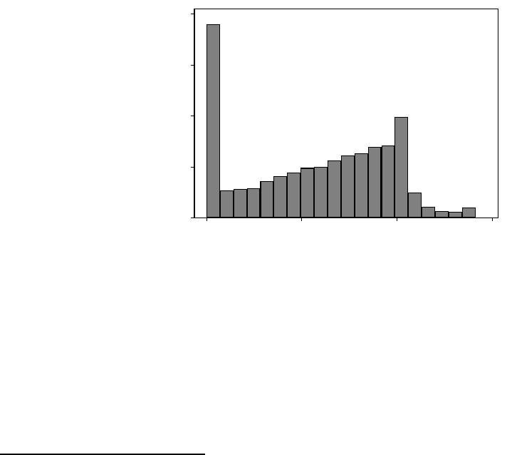
Figure 2 shows our sample distribution of LGD. Only 16 percent of the defaulted loans avoid

losses altogether, and 15 percent have losses of 100 percent or more. Had we constrained LGD to

be no higher than 100 percent, Figure 2 would look similar to the “U” shape seen in many

studies of realized losses.

We observe in our sample many loans with losses exceeding 100

percent. LDGs above 100 percent typically occur when expenses are significant and principal

recoveries are small. Such loans tend to be small (median EAD of $87,000, versus $260,000 for

the others), are more likely to be foreclosed (56 percent, versus 44 percent for the others), and

have longer workout periods (median of 11 quarters, versus 7 quarters for the others).

Figure 2: Sample Distribution of LGD

One contribution of our paper is that it uses a detailed measure of LGD that captures nearly the

full range of costs a lender would incur in resolving a defaulted ADC loan. Many studies of

losses on CRE mortgages are limited in their data on the composition of losses, and are limited to

comparing market price reactions to default announcements for CMBS securities or the

subsequent sales price of the property to loan exposure at default. We show in Figure 3 the

decomposition of LGD across different buckets of LGD losses. This breakdown shows how

expenses, the top (dark blue) segment in each column, account for a significant share of total

losses across the loss distribution. For loans with very small positive LGDs, expenses comprise

See Araten et al. (2004) and Asarnow and Edwards (1995) for examples of realized loss distributions.

1000

2000

3000 4000

Frequency

0 .5 1 1.5

LGD

more than 20 percent of losses. Charge-offs (COs) occasionally reflect the impact of successful

downstream recoveries. In some cases, they even offset some of the losses from expenses and

discounting, which is noticeable in the negative values for owned real estate charge-offs (ORE

COs) in the first three bars of Figure 3. For the segment with losses greater than 100 percent, the

share of expenses is approximately 17 percent of the total losses, highlighting the importance of

using loss measures that include expenses. The share of losses associated with charge-offs after

the bank has assumed ownership of the property—the ORE COs—increases as losses approach

and exceed 100 percent. ORE COs represents another 15 percent of the total losses for high LGD

loans in our sample, indicating that a significant portion of the total loss is being recognized later

in the workout process. LGD estimates that do not consider expenses related to assets in default,

or subsequent charge-offs for ORE assets, later in the workout are likely to underestimate the

extent of true losses incurred.

Figure 3: Decomposition of Net Losses by LGD Category

3.3 Descriptive Statistics

This section begins with basic descriptive statistics across the full sample. We then provide

additional detail on key variables and a breakdown of the sample based on geography and type of

collateral.

3.3.1 Full sample characteristics

As shown in Figure 4a, most of our loan originations occurred between 2005 and 2010, with 25

percent occurring in 2007 and 63 percent occurring between 2006 and 2008.

One interesting

aspect of the origination dates is that it includes a non-trivial share of construction loans

originated during the financial crisis, when overall construction lending dropped significantly.

Most defaults occurred between 2009 and 2011, with 33 percent in 2009, 29 percent in 2010, and

15 percent in 2011. This is clearly a sample of loans that defaulted during a period of severe

Observations where either the origination date or the default date are missing are excluded.

-20%

20%

40%

60%

80%

100%

20 30 40

50 60 70 80

90 100 130

LGD Category *

Expenses

Discounting

Loss on Sale

Net ORE COs

Net Loan COs

* 10 includes 1% < LGD =< 10%, 20 includes 10% < LGD =< 20%, etc. CO stands for charge-offs, net

of recoveries.

Source: FDIC

loss share and failed bank data.

distress, which is exactly when losses on construction loans are of greatest concern for lenders

and the broader economy.

Figure 4b shows the distribution of the term to maturity at origination. The mean term to

maturity is 4 years, and the mean age at default is 3.2 years.

In addition, 60 percent of the loans

are maturity defaults.

Assuming the project has progressed as expected, a default occurring at

maturity would suggest that a bank would have a complete or nearly complete project to seize as

collateral, instead of a partially complete project with greatly reduced value.

Figure 4a: Distribution of Origination and Default Date Figure 4b: Distribution of Term to Maturity

Figure 5 reports the distribution by asset size. The distribution is strongly skewed, with a large

number of smaller assets that relate to construction of individual single-family properties, and is

not dominated by large construction loans for single-family developments or large commercial

projects. This is due in part to the nature of the crisis itself, which was strongly associated with a

boom-bust cycle in single-family lending. It is also due in part to the nature of failed banks,

many of which were smaller institutions specializing in smaller single-family and commercial

construction projects rather than larger residential or commercial developments. It is possible, for

example, that the experience of builders or the structure of financing for those large-scale

projects could differ in certain ways from most of the defaulted loans in our sample. Our results

from this crisis should be interpreted with this in mind.

The average length of the loan is significantly longer than the time it takes to complete a single residential unit,

which is 7.8 months. The difference between the loan term and typical construction period reflects the additional

time built into the loan for preparation before vertical construction, the construction of multiple buildings financed

by the same loan, the construction of buildings with more than a single unit (where the average time to build is 17.4

months), and time required to sell the completed properties.

A maturity default is defined as a default that occurs within 90 days of the scheduled maturity or after maturity.

Figure 5: Sample Distribution of Asset Size

Table 1 reports descriptive statistics for the full sample. The first section of the table provides

data on the characteristics of the loans. The mean LGD is 56.7 percent, and the median is 62.4

percent. Defaulted loans with a positive loss for the lender make up 84.4 percent of the sample,

while 15.6 percent of the defaults resolve with no loss. As shown in Figure 5, the distribution of

the size of the loans is heavily skewed: although the mean exposure at default is $1.06 million,

the median is only $230,000. The median interest rate is 6 percent. And as mentioned previously,

the mean term to maturity at origination is four years, and the median is three years. The mean

age of the loan at default is about three years, and 60 percent are maturity defaults. About 37

percent of the sample was already in default when the originating bank failed, and 46 percent of

the loans were foreclosed during the workout period. The mean workout period is 25 months,

and it varies substantially across the sample. The legal process for foreclosure influences the

ability of lenders to seize assets and may be relevant to explain loan loss, so we look at whether

loans are in judicial foreclosure states (41 percent).

Construction lending is also an

informationally intensive business, where knowledge of local market conditions are important,

so we track whether loans are made outside of Core-Based Statistical Areas (CBSAs) in which

the originating bank has a branch presence (“out-of-territory”). About 25 percent of the loans

were made based on collateral located outside of the lender’s CBSA footprint; these are not

distributed evenly across regions or banks. For 9 percent of the loans, the outstanding loan

balance exceeded the initial loan amount at some point during the loss share period (thus

indicating that the acquiring bank authorized additional funds to minimize losses).

In judicial foreclosure states, foreclosure requires a court order.

Table 1: Descriptive Statistics for the Sample

The next section of the table looks at the characteristics of the banks in our sample. Growth in

the originating banks’ ADC portfolios was strong during the period leading up to origination: on

average, it was 36 percent in the previous year and 167 percent in the previous three years. The

mean CAMELS rating at origination is 2.49, and the median is 2. The mean size of the failed

banks at origination is $3.4 billion, and the median is somewhat less than $1 billion. We also

track the time the originating bank spends in distress (defined as having a CAMELS composite

rating of 4 or 5). If a bank is closed shortly after it begins to experience distress, then the loans

are more quickly transferred to a healthier institution, which may result in lower losses. In our

sample, the average time spent by the originating bank in distress is just over 1.5 years.

Variable

No. of

Obs

10th

Percentile

Median

90th

Percentile

Mean

Standard

Deviation

Basel LGD based on discounted loss share cash flows 19,427 0 0.624 1.015 0.567 0.383

1 if basel LGD has a nonzero loss 19,427 0 1 1 0.844 0.363

Loan Characteristics

Outstanding balance at default ($1,000) 19,427 31 230 2,658 1,056 2,598

Interest Rate 19,427 4.0 6.0 8.5 6.3 2.3

Term to maturity (years) 18,658 1.0 3.0 7.0 4.0 3.84

Age at default (years) 18,780 0.93 2.82 5.69 3.17 2.12

Maturity default* 18,661 0 1 1 0.60 0.49

In default when the bank failed 18,639 0 0 1 0.37 0.48

Foreclosed 19,427 0 0 1 0.46 0.50

Workout period (months) 19,427 3.5 23.5 50.4 25.3 17.9

Ratio of balance drawn to total exposure ** 19,427 1 1 1 0.95 0.14

Land development loan 9,286 0 1 1 0.89 0.32

Judicial foreclosure state 18,493 0 0 1 0.42 0.49

Out of territory loan (CBSA) 17,775 0 0 1 0.25 0.43

Overage (Asset bal > init exposure at any time) 19,427 0 0 0 0.09 0.29

Bank Characteristics

Bank 3-yr ADC loan growth rate at loan origination 19,427

1.25 4.00 1.67 1.42

CAMELS rating at origination 18,549 2 2 4 2.49 1.05

Asset size of failed bank at loan origination ($ millions) +

18,714 3,389 6,574

Failed bank time spent in distress (years) 19,427 0.45 1.18 2.10 1.27 0.66

Market Characteristics

Local ratio of ADC to total lending at origination 18,487 0.063 0.117 0.190 0.123 0.051

Local NC rate for ADC loans at origination 18,481 0.002 0.013 0.153 0.048 0.064

Local 3-yr change in ADC to total lending at origination 18,481 -0.026 0.025 0.075 0.024 0.042

Local 3-yr change in brokered to total deposits at orig 18,481 -0.020 0.022 0.058 0.020 0.041

One year pct point chg in SFR permits/total stock at orig 18,472 -0.004 -0.002 0.001 -0.002 0.002

Local average vacancy rate for CRE at orig 18,449 0.056 0.081 0.106 0.081 0.020

Local change in ADC to total lending (orig to def) 16,287 -0.090 -0.032 0.004 -0.037 0.038

Local NC rate for ADC loans at default 18,501 0.084 0.168 0.223 0.162 0.057

Change in local ratio of NC ADC to total loans 18,481 0.012 0.119 0.205 0.114 0.076

* Default was within 90 days of scheduled maturity or after maturity

** Capped at 100%

+ Percentile items omitted for privacy reasons

NC stands for noncurrent (including nonaccrual). SFR stands for single family residential.

A key focus of our paper is the degree to which local market characteristics can explain ADC

loan loss rates. The last section of Table 1 reports several market-level measures calculated from

the balance sheets of all banks with branches located in the CBSA where the loan’s collateral

resides. These measures are meant to reflect the general climate of ADC lending with respect to

other local lenders competing in that market space. Geographic allocations for loans from local

banks are based on CBSA-level branch shares as reported in the FDIC Summary of Deposits

(SOD).

Our sample is heavily weighted toward markets that experienced significant construction lending

growth. The average local ratio of ADC loans to total loans at origination is 12 percent, and the

average percentage point increase in this ratio over the three years before loan origination was 2

percent.

Interestingly, a significant share of the loans—22 percent— was originated when the

three-year change in the ratio of ADC loans to total loans was declining.

These loans also were

originated in areas where banks were aggressively seeking new sources of deposits, with the

ratio of brokered to total deposits increasing 2 percentage points, on average, during the three

years before loan origination. We interpret these local lending measures as a proxy for how

aggressive the competition may be from other local banks in the market and as a reflection of

local supply conditions.

We look at other measures of market conditions that relate new ADC lending to existing stock.

We use the one-year regional change in single-family permits to total stock at origination, which

averages -0.2 percent. A negative value is a forward-looking indication that growth in single-

family stock is slowing, while a positive value is a forward-looking indication that single-family

stock is increasing. A higher positive value at origination reflects markets in which the supply of

single-family housing is increasing more dramatically. The slower adjustment of construction

sector investment (arising from the time required to build) could exacerbate the mismatch

between demand and supply if demand decreases sharply post-origination, contributing to higher

losses in default. We also include the local vacancy rate by commercial property type at

origination, which averages 8.1 percent.

These rates show how much supply exists in the

market relative to demand for finished commercial properties when the loan is made. ADC loan

originations where vacancy rates are already high may be a sign of lenders originating into

markets with a lower capacity for future absorption when construction is complete, increasing

the losses in default should there be a negative shock to demand.

For context, contrast levels and changes of ADC lending for the Atlanta and Boston CBSAs during the period

leading up to the crisis. In Atlanta, the peak ratio of ADC loans to total loans was 19.3 percent; in Boston, it was 4.9

percent. In Atlanta, the average three-year percentage point increase in that ratio exceeded 3 percentage points from

March 2005 to September 2008, with a maximum of nine percentage points in March 2007; in Boston, it never

reached two percentage points.

About 40 percent of the loans were originated when the one-year percentage point change in ADC loans to total

loans was negative.

State-level data were used for loans outside a CBSA designation.

We also look at what happens in the local market between origination of the loan and default.

These variables relate to the risk ADC lenders face that local market conditions may change after

originating the loan and before construction is complete. The average change in the ratio of ADC

loans to total loans from origination to default is -3.7 percentage points. A decline in this ratio

indicates that lenders may be reducing exposures because they recognize markets are shifting

and they are adapting their lending volume to that risk. On the other hand, when this ratio is

increasing dramatically between the time of loan origination and default, there is a greater

chance that default is occurring in an overzealous or glutted market, and recoveries may suffer as

a result. Therefore, we expect higher losses in our sample if this measure is increasing between

origination and default. This variable differs from our inclusion of the local three-year change in

ADC lending to total lending in the lead up to origination in terms of when the information is

available to lenders. The three-year percentage point change in ADC lending before origination

could be considered part of the lender’s available information set when the loan is made.

However, the change in ADC lending between origination and default is a measure of the change

in ADC lending after loan origination, and would not be observable to lenders at origination.

While the former variable is tied to the extent to which lenders are managing their risk exposure

from excessive market growth, the latter highlights the risk faced by lenders in fast-growing

markets after origination, before the property may be completed and sold. We also look at the

ratio of noncurrent ADC loans to total loans at the time of default to get a sense of distress in the

local market. If a large share of local projects are in distress when the loan defaults, we expect

that the value of the collateral for a defaulted loan will be lower and the losses will be higher.

3.3.2 Segmented sample characteristics

We take a deeper dive into the data by looking at the sample segmented across different regions

and property types. Figure 6 provides a map of loan location counts by state, and Table 2

provides a breakdown of the sample by collateral type and location.

The sample is not highly

concentrated by bank. The largest bank (in terms of sample size) held 10.8 percent of the loans;

the top five held 24.7 percent.

We also report separately loans where, due to data quality issues, we could not identify the type of project.

Figure 6: Sample Location by State

Table 2: Sample Breakout by Collateral Location and Type

The sample is heavily concentrated both in the South and in loans collateralized by single-family

properties. Loans from the South comprise 61 percent of the sample, whereas those from the

Northeast comprise a mere 2 percent. At 28 percent of the sample, Georgia is the most heavily

represented, even though it accounted for only 3 percent of the U.S. population in 2007.

Several factors contribute to this feature of the sample. First, at the onset of the crisis, FDIC-

insured banks headquartered in the South were more heavily invested in ADC loans: as of year-

end 2007, institutions headquartered in the South held 40 percent of the total balance of ADC

FDIC loss share data and Census data.

Land/Dev Home Unknown

Multi-

family

Retail

Other/

Unknown

By State

Georgia 5,106 27.6% 1,704 463 1,263 67% 30 55 386 9% 1,205 24%

Florida 3,552 19.2% 1,911 54 529 70% 52 37 237 9% 732 21%

Illinois 1,490 8.1% 183 55 194 29% 353 31 276 44% 398 27%

California 1,226 6.6% 229 78 344 53% 140 45 84 22% 306 25%

Washington 986 5.3% 418 68 99 59% 63 33 51 15% 254 26%

All Other 6,140 33.2% 2,041 306 1,600 64% 137 180 473 13% 1,403 23%

By Region*

Northeast and Midwest 3,603 19.5% 691 155 722 44% 435 166 511 31% 923 26%

South 11,273 60.9% 4,568 611 2,585 69% 116 105 807 9% 2,481 22%

West 3,624

19.6%

1,227 258

722

61% 224

110

189 14% 894

25%

Total 18,500 100.0% 6,486 1,024 4,029 62% 775 381 1,507 14% 4,298 23%

Pct of Total 35% 6% 22% 4% 2% 8% 23%

No. of Obs

Pct of

Total for

Location

No. of

Obs

Pct of

Total for

Location

* The Northeast region is made up of Connecticut, Delaware, Massachusetts, Maine, New Hampshire, New Jersey, New York, Pennsylvania, Rhode Island, and

Vermont; the Midwest region is made up of Iowa, North Dakota, South Dakota, Illinois, Indiana, Michigan, Minnesota, Missouri, Nebraska, Ohio, Wisconsin, Kansas,

Oklahoma, and Texas; the South Region is made up of Alabama, Arkansas, Florida, Georgia, Kentucky, Louisiana, Maryland, Mississippi, North Carolina, South

Carolina, Tennessee, Virginia, District of Columbia, and West Virginia; the West region is made up of Arizona, California, Colorado, Idaho, Montana, New Mexico,

Nevada, Oregon, Utah, Washington, Wyoming, Alaska, and Hawaii. Northeast and Midwest regions are combined for privacy reasons.

Full Sample

Collateral Type

No. of

Obs

Pct of

Total

Sample

Single Family

Commercial

Unknown

No. of Obs

Pct of

Total for

Location

loans but only 28 percent of industry assets.

Second, institutions from the South and the West

failed and were resolved using the loss share program more often (South, 6.6 percent; West, 6.8

percent), whereas only 1.9 percent of banks in the Midwest and 0.9 percent of banks in the

Northeast failed and were placed into the loss share program.

In total, 47 percent of the banks

placed under the FDIC’s loss share program were headquartered in the South, 28 percent in the

Midwest, 22 percent in the West, and 3 percent in the Northeast. Moreover, the failed banks in

the Northeast had lower concentrations of ADC loans than those in other regions, and those in

the South had the highest concentrations.

Table 3 reports loan, bank, and market characteristics by region. Mean LGD is highest in the

South: 61 percent, versus 48 percent to 50 percent for the other regions. Loan sizes are much

smaller in the South, with a median value ($177,000) less than half that of loans in other regions

($326,000 to $500,000). The difference in loan size may reflect the higher share of loans in the

South that are collateralized by single-family properties. In most regions, maturity defaults

account for roughly 60 percent of all defaults, but in the Northeast they account for only 47

percent. However, the average draw rates suggest most of these projects drew almost all of their

committed balances even if they defaulted before maturity. Median interest rates on the loans are

slightly higher in the Midwest and West. Few states in the West are judicial foreclosure states,

while most states in the Northeast are. The share of loans where the asset balance at some point

exceeded the original committed balance is fairly consistent across regions, with a slightly higher

frequency observed in the South and the West.

There are strong regional patterns associated with out-of-territory lending by banks in our

sample. Loans collateralized by properties in the Midwest were the least likely to be out-of-

territory (13 percent), where there were a significant number of local bank failures but no boom

preceding the crisis. A strikingly large share of the loans in the Northeast were out-of-territory

(77 percent). There could be several reasons for this difference. First, there was no significant

real estate boom or bust there in the Northeast, and few local ADC lenders from that region

failed; thus, in our sample, lenders with loans in the Northeast tended to have higher shares of

out-of-territory loans than average. Second, construction may be more heavily constrained in the

Northeast because of zoning or less availability of suitable land for new development.

The originating failed banks in all four regions of our sample had high ADC loan growth at

origination, especially in the Northeast and West. When the sample loans were originated, the

Call Report data.

FDIC failure and Call Report data.

Failure rates are calculated as total failures placed under the loss share program

from 2008 through 2013 divided by total number of institutions as of year-end 2007. Puerto Rico banks had even

higher failure rates than what is reported for any of the regions reported here, but Puerto Rico is omitted because

loans from Puerto Rico are excluded from the sample.

Call Reports as of the quarter immediately before failure. The mean ADC concentrations were 13.2 percent for the

Northeast, 18.1 percent for the Midwest, 21.2 percent for the West, and 23.2 percent for the South.

Table 3: Sample Breakout by Region

lenders’ mean three-year ADC loan growth rate ranges from 146 percent in the South to 194

percent in the Northeast. All these rates exceed total industry growth: the industry’s peak three-

year growth rate for ADC loans during this period was 108 percent.

Banks that originated loans in the South were larger than in the other regions, with average assets

of $3.8 billion compared with $2.3 billion in the Northeast and $2.7 billion in the West and

Midwest. Banks that originated loans in the West spent the shortest average time in distress, just

over a year on average, while banks in the Midwest were in distress for 1.4 years on average.

The geographical pattern of loans in our sample reflects the conventional wisdom that

construction lending was the most aggressively competitive in the South and probably the least

competitive in the Northeast. This pattern can be seen in the greater increase in de novo lenders

in the South and the aggregate increase in concentration in construction loans in the South. The

estimated mean share of ADC to total loans at local competing banks at origination was 14

percent in the South, 10 percent in the West, 9 percent in the Midwest, and only 4 percent in the

Call Report data. The industry’s peak growth period ran from year-end 2003 to year-end 2006. The industry’s

quarterly growth rate peaked in June 2005 at 8.3 percent, started to decline in June 2006, and turned negative in June

2008.

Variable

Mean Median Std Mean Median Std Mean Median Std Mean Median Std

Basel LGD based on discounted loss share cash flows 0.61 0.69 0.38 0.48 0.48 0.40 0.48 0.51 0.36 0.50 0.53 0.41

1 if basel LGD has a nonzero loss 0.87 1 0.34 0.75 1 0.43 0.83 1 0.37 0.75 1 0.44

Loan Characteristics

Outstanding Balance at Default ($1,000) 757 177 1889 1155 326 2527 1897 500 3897 1678 345 3615

Interest Rate 6.18 6.00 2.17 6.40 6.50 2.14 6.82 6.50 2.65 6.63 6.25 2.05

Term to maturity (years) 3.53 2.96 3.04 5.94 3.85 6.04 3.76 3.02 2.93 4.68 3.47 3.44

Age at Default (years) 2.98 2.66 2.03 3.78 3.25 2.62 3.24 2.88 1.88 3.04 2.64 1.66

Maturity Default * 0.60 1 0.49 0.55 1 0.50 0.64 1 0.48 0.47 0 0.50

In default when the bank failed 0.37 0 0.48 0.33 0 0.47 0.42 0 0.49 0.48 0 0.50

Foreclosed 0.51 1 0.50 0.33 0 0.47 0.38 0 0.49 0.21 0 0.41

Workout period (months) 26.6 25.5 17.5 25.1 22.0 19.7 23.8 22.2 17.0 24.2 19.7 20.6

Ratio of balance drawn to total exposure ** 0.94 1 0.15 0.95 1 0.13 0.95 1 0.13 0.93 1 0.17

Land development loan 0.90 1 0.30 0.84 1 0.37 0.85 1 0.35 0.98 1 0.15

Judicial foreclosure state 0.44 0 0.50 0.65 1 0.48 0.07 0 0.25 0.85 1 0.35

Out of territory loan (CBSA) 0.25 0 0.43 0.13 0 0.33 0.28 0 0.45 0.77 1 0.42

Overage (Asset bal > init exposure at any time) 0.10 0 0.30 0.08 0 0.27 0.10 0 0.30 0.07 0 0.25

Bank Characteristics

Bank 3-yr ADC loan growth rate at loan origination 1.46 0.91 1.38 1.65 1.25 1.41 1.90 1.63 1.23 1.94 1.50 1.48

CAMELS rating at origination 2.65 2 1.12 2.30 2 1.01 2.18 2 0.74 2.32 2 0.72

Asset size of failed bank at loan orig ($ millions) + 3,855 7,435 2,727 5,188 2,775 4,825 2,332 4,814

Failed bank time spent in distress (years) 1.28 1.20 0.63 1.42 1.31 0.77 1.09 1.15 0.61 1.24 1.14 0.77

Market Characteristics

Local ratio of ADC to total lending at origination 0.143 0.140 0.046 0.090 0.087 0.030 0.099 0.086 0.050 0.037 0.030 0.020

Local NC rate for ADC loans at origination 0.057 0.017 0.069 0.039 0.013 0.054 0.029 0.009 0.049 0.022 0.016 0.025

Local 3-yr change in ADC to total lending at orig 0.025 0.034 0.048 0.017 0.019 0.025 0.028 0.024 0.033 0.013 0.012 0.011

Local 3-yr change in brokered to total deposits at orig 0.024 0.027 0.034 0.015 0.016 0.038 0.017 0.017 0.058 -0.022 -0.003 0.052

One year pct pt chg in SFR permits/total stock at orig -0.002 -0.003 0.002 -0.001 -0.001 0.001 -0.003 -0.004 0.003 -0.001 -0.001 0.001

Local average vacancy rate for CRE at orig 0.084 0.087 0.019 0.086 0.089 0.017 0.067 0.063 0.017 0.061 0.057 0.010

Local change in ADC to total lending (orig to def) -0.045 -0.041 0.041 -0.026 -0.024 0.027 -0.028 -0.024 0.032 -0.004 -0.001 0.014

Local ratio of NC ADC to total loans at default 0.165 0.173 0.051 0.152 0.153 0.061 0.168 0.170 0.066 0.111 0.113 0.046

Change in local ratio of NC ADC to total loans 0.107 0.112 0.074 0.113 0.119 0.078 0.139 0.149 0.079 0.090 0.090 0.046

* Default was within 90 days of scheduled maturity or after maturity

** Capped at 100%

+ Median omitted for privacy reasons

NC stands for noncurrent (including nonaccrual). SFR stands for single family residential.

South

Midwest

West

Northeast

Northeast. Banks in the South were also more aggressive in acquiring funds, with larger growth

in brokered deposits. The South exhibited a larger average decline in local ADC lending between

loan origination and default, suggesting a more dramatic correction in construction lending

supply during this period. The estimated increase in local ADC noncurrent rates was strong in all

regions, ranging from 9 percent in the Northeast to 14 percent in the West. However, the

noncurrent rates were lower at origination in the Northeast. At default, the estimated local

noncurrent rate for ADC loans exceeded 16 percent for the South and the West, 15 percent for

the Midwest, and 11 percent for the Northeast.

Table 4 repeats our analysis, breaking out the sample by project type instead of region. The

commercial ADC loans tend to be larger in size and with longer terms than single-family. They

also have a somewhat lower incidence of maturity defaults and out-of-territory originations. We

saw high growth in ADC loans at originating banks in the period leading up to loan origination

across all collateral types. For local ADC lending ratios, the average three-year change appears

somewhat higher in local areas for single-family collateral. In addition, brokered deposits grew

more in local areas in our sample where single-family loans were originated. Other measures of

local market conditions are largely consistent across collateral types.

Table 4: Sample Breakout by Project Type

Our sample is composed of loans originated (for the most part) during one real estate boom, and

defaulted and resolved during one period of distress. While similarities exist across real estate

and banking crises, certain characteristics are unique to each crisis. This period saw significant

Variable

Mean Median Std Mean Median Std Mean Median Std Mean Median Std Mean Median Std

Basel LGD based on discounted cash flows 0.58 0.66 0.39 0.51 0.48 0.35 0.56 0.59 0.37 0.52 0.55 0.38 0.59 0.67 0.38

1 if basel LGD has a nonzero loss 0.83 1.00 0.38 0.87 1.00 0.34 0.86 1.00 0.34 0.81 1.00 0.40 0.84 1.00 0.37

Loan Characteristics

Outstanding Balance at Default ($1,000) 857 175 2,264 848 248 1,817 677 193 1,701 1,795 499 3,673 1,355 315 2,960

Interest Rate 6.48 6.25 2.21 6.26 6.00 2.58 6.03 6.00 1.91 6.25 6.25 2.15 6.57 6.23 2.63

Term to Maturity (years) 4.26 3.56 3.17 2.80 2.45 2.33 3.15 2.75 2.76 5.65 3.50 5.93 3.74 2.92 3.89

Age at Default (years) 3.64 3.33 2.12 2.55 2.30 1.51 2.60 2.30 1.67 3.62 3.02 2.64 2.90 2.50 2.09

Maturity Default * 0.60 1 0.49 0.69 1 0.46 0.61 1 0.49 0.53 1 0.50 0.60 1 0.49

In default when the bank failed 0.29 0 0.46 0.50 1 0.50 0.43 0 0.50 0.36 0 0.48 0.42 0 0.49

Foreclosed 0.42 0 0.49 0.52 1 0.50 0.50 0 0.50 0.37 0 0.48 0.49 0 0.50

Workout period (months) 26.8 25.5 18.1 24.3 23.0 16.2 24.2 22.3 17.3 26.3 25.3 18.3 25.7 23.8 18.2

Ratio of balance drawn to total exposure ** 0.95 1 0.13 0.93 1 0.17 0.93 1 0.19 0.96 1 0.10 0.95 1 0.13

Judicial foreclosure state 0.47 0 0.50 0.19 0 0.39 0.35 0 0.48 0.48 0 0.50 0.41 0 0.49

Out of territory loan (CBSA) 0.26 0 0.44 0.23 0 0.42 0.24 0 0.43 0.21 0 0.41 0.25 0 0.43

Overage (Asset bal > init exposure at any time) 0.08 0 0.26 0.09 0 0.29 0.09 0 0.28 0.10 0 0.30 0.13 0 0.33

Bank Characteristics

Bank 3-yr ADC loan growth rate at loan orig 1.44 1.10 1.28 1.56 1.24 1.27 1.53 0.93 1.42 1.84 1.49 1.46 1.71 1.27 1.39

CAMELS rating at origination 2.48 2 1.04 2.54 2 1.08 2.59 2 1.11 2.39 2 1.02 2.48 2 1.03

Asset size of failed bank at loan orig ($ millions) + 3,285 6,400 1,296 921 4,531 7,822 1,920 3,857 3,998 7,451

Failed bank time spent in distress (years) 1.38 1.31 0.70 1.23 1.26 0.70 1.19 1.18 0.70 1.35 1.30 0.63 1.13 1.18 0.54

Market Characteristics

Local ratio of ADC to total lending at origination 0.128 0.122 0.049 0.131 0.133 0.049 0.124 0.123 0.052 0.104 0.092 0.047 0.123 0.116 0.053

Local NC rate for ADC loans at origination 0.046 0.010 0.064 0.056 0.021 0.063 0.053 0.016 0.068 0.048 0.014 0.064 0.044 0.014 0.058

Local 3-yr change in ADC to total lending at orig 0.025 0.029 0.043 0.029 0.035 0.043 0.021 0.024 0.046 0.019 0.020 0.036 0.027 0.025 0.036

Local 3-yr change in broker to tot deposits at orig 0.023 0.024 0.043 0.023 0.026 0.038 0.018 0.022 0.045 0.013 0.016 0.035 0.023 0.024 0.039

One yr pct pt chg in SFR permits/tot stock at orig -0.002 -0.002 0.002 -0.002 -0.003 0.002 -0.002 -0.003 0.002 -0.002 -0.002 0.002 -0.002 -0.003 0.002

Local average vacancy rate for CRE at orig 0.080 0.078 0.020 0.085 0.091 0.021 0.082 0.084 0.020 0.083 0.086 0.019 0.079 0.079 0.020

Local change in ADC to total lending (orig to def) -0.046 -0.041 0.040 -0.041 -0.037 0.037 -0.032 -0.026 0.036 -0.035 -0.031 0.034 -0.030 -0.025 0.036

Local ratio of NC ADC to total loans at default 0.163 0.169 0.057 0.171 0.184 0.052 0.154 0.160 0.057 0.171 0.180 0.053 0.160 0.166 0.058

Change in local ratio of NC ADC to total loans 0.117 0.126 0.080 0.115 0.121 0.076 0.101 0.104 0.072 0.123 0.134 0.076 0.116 0.115 0.073

* Default was within 90 days of scheduled maturity or after maturity

** Capped at 100%

+ Medians omitted for privacy reasons

NC stands for noncurrent (including nonaccrual). SFR stands for single family residential.

SFR land

SFR homes

SFR (stage unknown)

Commercial

Unknown

expansion in the supply of single-family housing before the crisis, but less of an expansion for

commercial properties. The next real estate crisis will probably play out differently.

4. Methodology

We implement a two-step estimation approach in our analysis to accommodate the bimodal

nature of the LGD data. As shown in Figure 2, the observed distribution is a mixture of discrete

and continuous outcomes, with a discrete spike at zero representing defaulted loans that

experience no loss and a continuous portion above zero representing the severity conditional

upon incurring a loss.

The two-step model distinguishes between discrete and continuous

portions of the LGD distribution, and it allows the underlying process to differ between them.

This helps disentangle the two channels of loss probability and loss severity in the different

modes of the LGD distribution. As observed in Schuermann (2004), “Defaults resulting in 100

percent recovery (0 percent LGD) are probably somewhat special and should be modeled

separately. Put differently, it is likely that there may be different factors driving this process, or

that the factors should be weighted differently,” (p. 270). Versions of the two-step approach have

been used elsewhere in the existing LGD literature; examples include Matuszyk (2010), Bellotti

and Crook (2012), Leow and Mues (2012), Loterman et al. (2012), Leow et al. (2014), Hwang et

al. (2016), Tanoue et al. (2017), Do et al. (2018), and Do et al. (2019).

In the first step of the model, we estimate the probability of falling into either mode of the LGD

distribution: Pr

(

 = 0



)

and Pr

(

 > 0



)

, where y represents observed values of LGD and x is

the vector of covariates. In the second step, we estimate the loss severity conditional upon falling

into the loss mode of the distribution, where we assume that  follows a log-normal distribution

for observations where  > 0. If we generalize Pr

(

 > 0



)

= () as the cumulative

distribution function (typically chosen from either a probit or logit distribution), and () as

the appropriate density for | > 0, then the log-likelihood contribution for observation  is

written as



[





(



)]

= 1

[





= 0

]



[

1 − ()

]

+ 1[



> 0][()()]

where  is the vector of covariates, and  and  are the estimated parameters of their respective

functions. The MLE of  for the binary loss outcome can be a probit or logit estimator. The MLE

of  for loss severity is the OLS estimator, which we specify as a regression of () on ,

conditional on  > 0. The two steps can be estimated separately since the parameters are

additively separable in the log-likelihood function; see Belotti et al. (2015).

While the spike at zero may resemble a censored distribution, these are actual observed zero losses conditional on

default rather than the product of a censoring constraint. As the entire distribution of LGD is observable, no

correction for selection bias is needed. See Leung and Yu (1996) and Belotti et al. (2015) for further detail on the

two-step approach; Wooldridge (2010) provides useful discussion as well; see Chapter 17, pp. 690-692.

The results from the two estimation steps may then be combined to attain the overall marginal

impact of the covariates on LGD. The expected value for LGD then is not a simple mean, but is

weighted by the probability of incurring loss

(|) = ( > 0|)(|,  > 0)

where ( > 0|) = (’)/

[

1 + 

(

’

)]

is from the first-step logit regression and

(|,  > 0) = (’ + 

/2) is from the second-step log-linear regression.

Coefficients are reported for the first-step logit and second-step linear regressions, as well as for

the combined marginal effects on LGD. For all regressions, standard errors are clustered at the

level of the originating bank. Because we expect that LGD will behave differently for loans

collateralized by single-family and commercial projects, we run separate sets of regressions for

each collateral type.

As detailed in Section 3.3, we observe variation in our sample at the level of the individual loans

in default, the failed banks originating the loans, and the local markets in which the loan

collateral is located. Loan-level characteristics include basic information on the individual loans

that may be known at origination (such as the amount of committed exposure and whether the

collateral is out-of-territory), but also certain later indications (like cost overruns) suggesting that

the construction process may have run into trouble. Characteristics of the failed bank (such as

growth rates at origination or time spent in distress before failure) could reflect shared qualities

on loans related to origination practices or management troubles at the originating institution.

Finally, conditions in the local markets—both at origination and at default—may inform about

factors like local loan supply or default trends that could affect the value of recoveries in default.

To highlight the relative importance of these categories, we estimate our regressions using the

following general format: LGD=f(Loan characteristics, Originating bank characteristics,

Market characteristics).

5. Results

We present the results from our analysis by discussing the impact of the loan characteristics in

Section 5.1, the bank characteristics in Section 5.2, and the market characteristics in Section 5.3.

Section 5.4 presents an analysis of counterfactuals to shed additional light on the core results,

and Section 5.5 discusses robustness testing.

Our primary results are shown in Table 5. Columns 1–3 provide single-family results and

columns 4–6 provide commercial collateral results. For each collateral type, the logit model is

shown first (columns 1 and 4), then the GLM results for assets with positive losses (columns 2

and 5), and then marginal effects that combine the logit and GLM results (columns 3 and 6).

Table 5: Primary Regression Results

Single- Family ADC Loans

Commercial ADC Loans

(1)

(2)

(3)

(4)

(5)

(6)

Logit

GLM

Margin

Logit

GLM

Margin

Loan level variables

Land development loan

-0.039

0.250***

0.137***

(-0.229)

(4.712)

(4.239)

Exposure at default (log)

0.183***

-0.070***

-0.026***

0.329***

-0.067***

-0.007

(4.841)

(-7.810)

(-4.143)

(5.576)

(-5.944)

(-0.903)

Judicial foreclosure state

0.307**

0.080**

0.067***

-0.041

0.148***

0.071***

(1.982)

(2.228)

(2.996)

(-0.228)

(4.707)

(3.337)

Out of territory loan (CBSA)

0.321**

0.031

0.041**

-0.034

-0.006

(2.078)

(1.146)

(2.142)

(-0.164)

(-0.169)

(-0.236)

Balance drawn / total exposure

-1.709

-1.136**

-0.760***

1.859

-3.239***

-1.483**

(-1.092)

(-2.401)

(-2.622)

(0.622)

(-3.035)

(-2.471)

Balance drawn / total exposure,

Squared

2.498**

0.792**

0.627***

0.284

2.136***

1.103***

(2.048)

(2.382)

(3.011)

(0.131)

(2.837)

(2.605)

Overage

0.553**

0.111***

0.103***

1.213***

0.090***

0.146***

(2.305)

(4.900)

(4.814)

(3.344)

(2.8138

(4.236)

Loan age at default (quarters)

-0.042***

-0.016***

-0.012***

-0.041***

-0.011***

-0.009***

(-3.302)

(-7.582)

(-8.052)

(-5.479)

(-5.180)

(-7.259)

Maturity default

-0.633***

-0.049***

-0.074***

-0.023

-0.006

-0.005

(-5.823)

(-3.225)

(-6.316)

(-0.131)

(-0.250)

(-0.263)

Bank level variables

3-year growth ADC to total

lending at origination

0.115*

0.026***

0.023***

0.184***

0.014

0.022***

(1.856)

(2.718)

(3.237)

(3.143)

(1.246)

(3.179)

Asset size (log)

-0.152***

-0.019**

-0.022***

-0.128*

-0.014

-0.018**

(-3.169)

(-2.033)

(-3.546)

(-1.752)

(-1.189)

(-2.144)

Time in distress (quarters)

-0.023

0.009**

0.003

-0.016

0.027***

0.013***

(-0.748)

(2.093)

(0.983)

(-0.376)

(4.510)

(2.691)

Market level variables

Local ADC to total loans at

Origination

5.595*

0.266

0.562*

14.774***

0.987**

1.725***

(1.906)

(0.597)

(1.692)

(4.332)

(2.030)

(4.665)

Local 3-yr growth ADC to total

loans at origination

9.504***

2.319***

1.998***

-0.417

2.349***

1.153***

(3.509)

(5.031)

(6.118)

(-0.155)

(4.339)

(3.249)

Local 3-yr change brokered to

total deposits at origination

0.841

0.585**

0.389

2.097

0.515

0.434*

(0.312)

(2.554)

(1.642)

(1.045)

(1.266)

(1.646)

1-yr change SFR permits to

total housing stock at orig

19.555

22.139***

13.804***

94.538**

10.625

13.220**

(0.549)

(4.308)

(3.497)

(2.125)

(1.198)

(2.292)

Local CRE vacancy rates by

property type at origination

7.512**

1.311**

1.288***

3.402

3.415***

2.009***

(2.251)

(2.003)

(2.879)

(0.735)

(4.419)

(3.720)

Change in local ADC to total

loans (origination to default)

8.595***

2.179***

1.852***

13.363***

3.774***

3.017***

(2.761)

(4.193)

(5.054)

(3.456)

(6.015)

(6.842)

Local noncurrent to total ADC

loans at default

1.220

0.670***

0.464**

-1.314

0.970***

0.381*

(0.674)

(2.602)

(2.356)

(-0.690)

(3.571)

(1.787)

Constant

0.494

0.777***

-3.580**

1.178***

(0.357)

(3.410)

(-2.474)

(2.774)

Observations

6,414

5,351

6,414

2,399

1,934

2,399

Pseudo R-square

0.138

0.360

0.216

0.143

0.365

0.214

T-statistics are shown in parentheses under the parameter estimates. Standard errors are clustered

at the level of the originating bank.

5.1 Loan Characteristics

For single-family collateral, we find that land and land/lot development loans have consistently

higher LGDs.

These loans experience a marginal increase of 13.7 percentage points for LGD

relative to loans backed by completed homes. The result is consistent with other authors’

findings that pricing is more volatile for projects in less complete stages; see Nichols, Oliner, and

Mulhall (2013), for example.

We find consistent evidence that loan size matters for both collateral types, with smaller loans

resulting in higher LGDs. Studies of LGD for CRE loans have found mixed evidence regarding

loan size;

however, most other studies examine loans much larger than those in our sample,

and thus may not be comparable in this respect. The median size of the loans in our sample is

small ($230,000), and as noted in Section 2.1, the loan administration processes for ADC loans is

more complicated than for other loan types. Therefore, fixed costs of the workout process

probably explain some of these differences. For both collateral types, smaller loans in default are

less likely to have positive losses, but the positive loss rates are higher when they occur. It may

be that a larger share of the small loans is owner-occupied. Borrowers that occupy the property

probably have information advantages over other borrowers, and they may be more highly

motivated to address problems effectively so that they can retain control of the property. Thus,

the weakened incentives associated with borrowers with negative equity positions may be less

important for owner-occupied projects. Another factor could be the prioritization for lenders

themselves, who may more intensely focus their recovery efforts and limited resources on larger

loans to minimize the total amount of losses in their portfolios.

Likewise, loans in judicial foreclosure states consistently have higher LGDs for both collateral

types. Judicial foreclosure laws require lenders to go through the courts to foreclose on a

property, adding both time and cost to the foreclosure process. In addition, borrowers may well

be able to leverage their knowledge of these additional costs when negotiating with lenders.

The majority of previous analyses on the impact of judicial foreclosure has been focused on how

We also estimated a Tobit specification of our model, with results that were consistent with the two-step

specification. We believe that the two-stage approach reported here provides a better way to parse the bimodal

variation in losses that we observe and also provides a better statistical fit of the data.

We are unable to test for the significance of land/lot development loans for the commercial sample because this

detail was not collected for commercial ADC loans in the Loss Share Administration data. We believe there are

likely to be fewer land/lot development loans in the commercial ADC loan sample than in the single-family sample.

We are told by industry experts that many of the commercial loans tended to be closer to the city center on

established rather than new lots.

Schuermann (2004) surveys the literature for CRE loans and concludes that asset size probably does not matter;

Pendergast and Jenkins (2003) and Asarnow and Edwards (1995) find lower LGDs for larger loans.

Shibut and Singer (2015) found that LGD, workout periods, and expenses were all higher for judicial foreclosure

states, regardless of whether the loan was foreclosed. See Table 5 in that paper.

they change the incentives for lenders and borrowers, resulting in lower loan originations in

Pence (2006) or more strategic defaults in Ghent and Kudlyak (2011). The impact of judicial

foreclosure laws on loans to homebuilders may differ from those on homeowners. An et al.

(2013) look at the impact of judicial foreclosure on CMBS loans. Kyle and Binder (2019), using

bank loan data, find little correlation between the use of recourse on CRE loans and the presence

of judicial foreclosure laws.

Single-family ADC loans made out-of-territory for the originating bank had higher losses.

However, we do not see a similarly significant effect for commercial ADC loans that were out-

of-territory. More than two-thirds of the out-of-territory single-family loans in our sample were

made in the South, compared with slightly more than half for commercial collateral. The South

experienced significantly higher proportions of ADC lending to total lending at origination,

higher growth in brokered deposits at origination, and a more dramatic pullback in lending

between origination and default, suggesting greater volatility in local markets. It is possible that

out-of-territory lenders would have had greater difficulty monitoring loan performance and

managing downside risks under those conditions.

While the preceding loan-level variables are set at the time of loan origination, the next several

variables in our model relate to the performance of the borrower/builder after origination, the

monitoring function of the lender, and the creation of collateral value for ADC loans over the

loan term. Our model includes the age of the loan at default (to identify loans that got into

trouble early on), the draw rate and squared draw rate at default (to measure progress via funds

disbursed relative to total amount committed), a maturity default indicator (for construction that

may be complete or near complete), and an overage indicator (for additional funding increasing

the lender’s exposure in an effort to minimize losses). These variables capture developments in

the construction process after the loan is originated, highlighting the critical nature of loan-level

risks for ADC loans after origination. In addition, these variables relate to risk with respect to

collateral creation over the life of the ADC loan, with the idea that projects defaulting sooner and

in a less complete state may tend to have lower collateral recovery values relative to completed

collateral.

Loans backed by single-family or commercial projects that do not default until a large share of

the balance is drawn—usually indicating most of the construction is complete—tend to have

lower LGDs. This can be seen by the negative coefficient on the ratio of balance drawn to total

exposure, or the draw rate. As builders are permitted successive draws on the loan, and as the

collateral construction progresses further, the collateral property itself may have greater recovery

potential for the lender. The positive coefficient on the squared term suggests that this effect is

strongest in the early stages of construction and diminishes as the draw rate increases. Loans

with overages tend to have higher losses, seen in the positive and significant coefficient on the

overage variable, but will also tend to have a higher balance drawn at default than other loans at

a similar stage of construction. Overages probably signal problems with either the initial estimate

of construction costs, the construction process, or both, which would partially counter the

observed negative effect on LGD for higher draws. In addition, there may be more noise in terms

of construction progress and costs incurred when observing later stages of construction with

higher draw rates on the loan. Hence, we see a nonlinear negative relationship between balance

drawn and LGD that diminishes for higher draws. Further, there is a difficult tradeoff in

uncertain outcomes for lenders, between the higher value of a project closer to completion and

higher losses on poorly managed projects that were not cut off when they should have been. The

ability of lenders to monitor projects effectively and make good decisions with respect to this

tradeoff appears to be an important consideration in managing losses on ADC portfolios.

The age of the loan, or the time between loan origination and default, also shows consistent

patterns across collateral types. Our results indicate that loans defaulting later in the life of the

loan tend to incur smaller losses. This is different from our inclusion of the draw rate, which is

meant to reflect the state of progress on the loan and the creation of collateral value. Rather, the

age of the loan is meant to capture loans that get into trouble quickly, reflecting severe problems

in the origination or construction processes that become evident fairly soon after origination.

We considered defining this variable as a ratio of the age of the loan at default to the term of the

loan, due to relative differences in term lengths across loans. However, our intent here was not so

much to reflect relative progress on the loan, particularly since we already include the draw rate

at default, which we believe better captures the progression on the loan. Rather, we expect that

early defaults would generally be weaker projects, and hence incur greater losses.

We find that maturity defaults tend to have lower LGDs for single-family projects, with a

marginal decrease of 7.4 percentage points; the relationship is insignificant for commercial

projects. Maturity defaults are somewhat more common for single-family (61 percent, versus 54

percent for commercial). However, the term defaults appear to perform more poorly for single-

family than for commercial collateral, both in the incidence of non-zero losses (88 percent versus

79 percent) and the severity of non-zero losses (73 percent versus 67 percent). It could be that

banks use simpler measures to determine default for single-family projects (which tend to be

smaller), and thus only the worst single-family loans become term defaults. Commercial projects

are larger and thus could merit more substantial monitoring, resulting in defaults being identified

more promptly when minor problems arise. In addition, the construction process for single-

The age of the loan at default and the draw rate are not highly correlated; in fact, the correlation within our sample

is slightly negative (ρ=-0.09). Loans with shorter terms by nature would not reach the higher age at default that

longer-term loans might sometimes attain; they might also tend to be further along in a relative sense in their rate of

draws within the shorter window of term. Even defining the age at default as a ratio relative to the term of the loan,

age is not highly correlated with the draw (ρ=-0.03). For example, in the event of a construction delay, the age of the

loan would still advance, while the draw rate would not. In addition, cost overruns and overages may be reflected in

the draw but not necessarily the age at default relative to loan term. This is consistent with our interpretation of

different information reflected in the draw and the age variables for the regressions.

family projects may be simpler, so it may be less likely that covenant violations trigger default

before maturity for single-family loans.

In summary, a strong relationship exists between loan characteristics and LGD. ADC loans are

not monolithic: bank choices about the types of ADC loans that they originate and their

monitoring practices have a big effect on distressed LGD. Further, the variables in our model

concerning post-origination performance highlight the risk in ADC lending throughout the life of

the loan and with respect to collateral value creation over the loan term. They also point to the

importance of bank monitoring efforts, given the inherent construction and collateral risks

involved for individual ADC loans.

We were unable to test certain loan attributes because of a lack of data. These attributes include

the experience of the lending officer and the builder, which Lusht and Leidenberger (1979) find

to be important for default, and details on the origination process, such as the type of capital

contribution (cash or real estate) and the type of appraisal used for valuation.

In addition, we

lack direct measures of the quality of loan monitoring, which may matter for LGD as well.

5.2 Originating Bank Measures

We find that three items related to the lender at origination inform LGD. First, we find that the

lender’s three-year growth rate for ADC loans to total loans during the period leading up to

origination is positive and statistically significant. Lenders who have rapidly expanded in ADC

lending—and thus have high growth rates—may have less experience managing the unique risks

associated with ADC lending that a bank who has a more mature ADC lending operation. We

control for the local three-year growth rate for ADC loans to total loans to ensure that we are

capturing differences in bank behavior and not merely differences in local lending conditions.

We find that the size of the lender at origination matters, but the relationship is relatively modest.

At the mean, an increase in bank size by 50 percent at origination is associated with a 1.1

percentage point decrease in LGD for single-family collateral and a 0.09 percentage point

decrease for commercial collateral. Small banks are more likely to experience positive losses,

and they tend to experience a higher loss severity for loans funding single-family development.

This result may relate to the bank’s resources and capacity to manage a troubled loan portfolio.

We examine whether the effect could be driven by the de novo banks in our sample, which are

significantly smaller (averaging just over $200 million in assets, compared to over $3 billion for

other banks). However, we find that including a control for de novo banks does not change the

significance of bank size for LGD. We also find that performing separate regressions for de novo

Some loan characteristics are important to LGD for other loan types but are not very relevant for ADC loans. This

includes the seniority of the debt level (almost all ADC loans are first liens) and, for commercial and CRE loans,

industry type and the financial condition of the borrower’s industry. Almost all of these loans have the same industry

type (construction), and many of the commercial properties are either multifamily (thus have no industry) or could

meet the needs of tenants from multiple industries.

banks and non de novo banks reveals a bank size effect for both populations. It is possible that

small banks, regardless of age, may feel pressure to grow in certain markets when competition is

high. This may affect the lending decisions, the resources available to monitor and work out a

distressed loan portfolio, and the losses incurred when markets turn.

In addition, the time that the lender spent in distress before its failure also has a modest effect.

For loans secured by single-family collateral, time in distress is associated with loss severity only

for loans with positive losses. For loans secured by commercial collateral, the overall marginal

effect is positive and strongly significant. This measure probably relates to the bank’s ability to

service loans effectively, especially the larger, more complex loans used to finance commercial

projects. Many troubled banks may face staffing disruptions and constraints that prevent them

from effectively managing their loan portfolios.

We test measures of bank health at origination and found them to be insignificant. Although all

of these banks failed, they were generally healthy at origination. The median equity ratio of these

banks at origination was 8.5 percent, the median composite CAMELS rating was 2, and the

median percentage of ADC loans that were noncurrent was 1.6 percent.

5.3 Local Market Measures

We find compelling evidence that local markets—both at origination and default—play an

important role in LGD. We discuss measures as of the time of origination and then measures

related to default.

5.3.1 Factors at Origination

For both collateral types, we find relationships between LGD and the local ratio of ADC loans to

total loans at origination, as well as the local three-year change in ADC loans to total loans at

origination. For loans secured by single-family collateral, the local share of ADC loans to total

loans is associated with only the probability of positive losses and is significant only at the 10

percent level. For commercial collateral, the relationship is much stronger, both in the size of the

effect and the statistical significance.

The local three-year change in the ratio of ADC loans to

total loans has very strong marginal effects: a one standard deviation increase in the ratio is

associated with an 8.4 percentage point increase in LGD for loans backed by single-family

collateral and a 4.8 percentage point increase for loans backed by commercial collateral. Both of

these factors relate to the strength of local market competition when the loan is originated, which

can increase risk exposure through multiple channels, including weaker loan underwriting, less

experienced lending staff, and higher potential for overbuilding.

As another measure of the state of local markets at origination, we include the three-year change

in the ratio of brokered deposits to total deposits in the originating bank’s local footprint. Our

A one percentage point increase in the ratio results in a 1.9 percentage point increase in LGD.

regressions provide some evidence that the local share of brokered deposits can be associated

with higher losses. We interpret a large inflow of brokered deposits into local banks as an

indication of demand for ADC loans outpacing local core deposit availability, and where markets

may be more likely to show signs of overheating. We also test brokered deposit ratios and

growth rates at the originating bank to see if these measures point to riskier behaviors and higher

losses, but we did not find significant results. Thus, it does not appear that banks with a higher

level of brokered deposits necessarily had worse LGD outcomes, but rather loans that were made

in areas with more brokered deposits rushing in had worse LGD outcomes.

The change in single-family permits to total housing stock focuses on expected increases in new

buildings compared to the existing housing stock, a forward-looking measure of new

construction that will be coming onto the market. We find a significant and positive association

with LGD. ADC projects that are originated when this measure is increasing strongly may be

coming online at completion in markets that are much more saturated than when the loans were

originated. The risk of oversupply in these markets may be greater, with higher losses on loans in

default.

We also include CBSA-level vacancy rates by commercial property type at origination.

This

measure reflects the condition of the local CRE market at origination and how well the existing

supply may be accommodating the demand for real estate. We anticipate that a higher vacancy

rate at origination may indicate supply outpacing demand, and for higher losses to occur in

default. Like the single-family permits, its marginal effect is large and strongly significant in

both collateral types for loss severity. A one percentage point increase in the vacancy rate at

origination is associated with a 1.3 percentage point increase in LGD for single-family collateral

and a two percentage point increase for commercial collateral. Substituting commercial vacancy

rates at default instead of at origination also matters for LGD, but we found a stronger

association with LGD for vacancy rates at origination; a high correlation between the two

precludes us from including both in the regression specification. Our interpretation would differ

somewhat between them; we interpret the vacancy rate at origination as reflecting the

information set for banks when the lending decision is made, and may inform forward-looking

expectations of where the market for new completions may be headed. The vacancy rate at

default, on the other hand, reflects the state of the market when the loan defaults, with

implications for collateral valuation when the recovery efforts are beginning.

Looking across local market measures at origination, we find multiple factors related to the local

environment at origination that are strongly related to LGD—losses that are realized later. No

single item encompasses all aspects of the local market at origination, but the overall strength of

these measures confirm that local market conditions at origination matter a great deal for LGD.

CoStar. For loans in our sample where the property type was unknown, we used an average of the local CBSA-

level vacancy rates for retail, office, and multifamily.

5.3.2 Factors at Default

Our model includes two items related to local market conditions associated with default: the

change in the share of ADC loans to total loans for local banks between origination and default,

and the noncurrent rate for local banks at default. The change in the local share of ADC loans to

total loans is very strong for both collateral types. For loans backed by single-family projects, a

one percentage point increase in the ratio is associated with a 1.9 percentage point increase in

LGD; for commercial collateral, three percentage points. As discussed previously, there are

multiple channels through which oversupply issues might increase LGD. Glutted markets are

likely to trigger fire sales or lengthy and expensive delays in the sale as lenders wait for markets

to recover. The oversupply is likely to exacerbate the divergence of incentives between the bank,

the builder, and the investor, resulting in increased losses for the bank. Potential tenants may

prefer not to move into new buildings because they can negotiate lower rates from existing

landlords and avoid the cost of moving, or they may only be coaxed into moving with highly

advantageous rents that reduce the value of the collateral.

Our second measure, the estimated local ADC noncurrent rate at default, is also significant for

LGD, but to a lesser degree and with less statistical significance than the change in local ADC

lending between origination and default (95 percent for loans backed by single-family projects;

90 percent for commercial). A one percentage point increase in the local noncurrent rate is

associated with a 46 basis point increase in LGD (single-family) and a 38 basis point increase

(commercial). Note that the local ADC noncurrent rate at default varies considerably across the

sample: the standard deviation is 5.7 percentage points, so a one standard deviation change is

associated with a LGD change of 2.7 for single-family collateral and 2.2 percentage points for

commercial collateral.

We consider but reject items measured as of the end of the workout period

or over time periods

that end when the loan cures or the asset is extinguished. We believe that the length of the

workout period is endogenous for the model, so its use would bias our results.

5.4 Counterfactual Analysis

In this section, we use two methods to study the sensitivity of LGD to loan-level, bank-level, and

local market-level variables. In the first analysis, we determine whether high or low values of

each regressor tend to reduce LGD (designated as “good”) or increase LGD (“bad”). To

determine the effects of the loan variables, we apply the marginal effects at the “good” and “bad”

percentiles (25

and 75

as appropriate) for only the loan-level variables; we assume the median

value for the remaining variables. We follow the same procedure for the bank-level and market-

level variables. We also break down the market variables into those at origination and after

The same basic idea also applies to potential buyers.

The workout period is defined as the period between default and the cure date or the date the asset is extinguished.

origination, because the implications differ for these subgroups. We do this separately for single-

family and commercial ADC loans, and we compare the relative dispersions in estimated LGD.

Table 6 provides results.

Table 6: LGD Effects by Collateral Type

The difference in expected LGD between loans with “good” and “bad” loan-level characteristics

is large: 33.5 percentage points for single-family collateral and 19.4 percentage points for

commercial collateral. Likewise, the effects of markets are very strong, with swings of 32.2

percent for SFR and 37.3 percent for commercial. The effects for individual bank-level

characteristics are smaller (respectively 8.4 percent and 13.5 percent). We also find that the

effects of markets, both at and after origination, contribute significantly to LGD.

The originating banks themselves exert indirect control over the loan characteristics to some

extent. Some loan characteristics, such as those tied to the location of loan, are static and known

at origination. They cannot be changed by the bank but can enter into the bank’s decision to

originate the loan in the first place. Other loan characteristics can change over the life of the loan

and are at least partly dependent on the ability of the bank’s monitoring function to flag potential

issues. Given the importance of the monitoring function in construction lending, we break the

loan characteristics into those that are static and known at origination, and those that may be

influenced in part by the loan monitoring function. Static loan characteristics in our model that

are known at origination include the size of the loan, location in a judicial foreclosure state, out-

of-territory status, and whether it is a land/lot development loan. Characteristics that are partly

influenced by the monitoring function include the age of the loan at default, the ratio of the

amount drawn to amount committed, term versus maturity default status, and whether an overage

was granted to the borrower.

Good

Bad

Difference

Single Family

Loan Characteristics

43.6%

77.1%

33.5%

Bank Characteristics

51.8%

60.2%

8.4%

Market Characteristics

at Origination

48.0%

67.0%

19.0%

after Origination

49.9% 62.7%

12.8%

Total

42.4%

74.6% 32.2%

Commercial

Loan Characteristics

43.2%

62.6%

19.4%

Bank Characteristics

44.3%

57.8%

13.5%

Market Characteristics

at Origination

40.8%

61.2% 20.4%

after Origination

43.9% 60.3%

16.4%

Total

34.4%

71.7%

37.3%

To explore the extent to which these non-static loan variables may be picking up on bank-level

policies and behaviors, we repeat the above analysis using bank-level fixed effects instead of

bank characteristic variables. Bank fixed effects will not inform us about specific relationships

between bank characteristics and loan losses, but the intent here is to absorb as much of the

bank-level explanatory power as possible via these fixed effects. This gives us a closer

approximation for how much these non-static covariates on the loan should be interpreted as

individual borrower/builder-driven versus bank-driven.

Since banks may target ADC lending

of a particular type (i.e., single-family or commercial), we again examine the subgroups

separately by collateral type in Table 7. Market-level variables are included in these

specifications, as in the prior analysis, but are not reported the Table in order to focus more

concisely on loan characteristics.

Table 7: LGD Effects by Collateral Type, with Bank Fixed Effects

Table 7 shows that bank-level fixed effects only slightly decrease the sensitivity of LGD to loan

characteristics. We estimate a difference of 31.8 percentage points in LGD between “good” and

“bad” loan-level specifications for single-family collateral, relative to 33.5 percentage points

incorporating bank variables but not bank fixed effects in Table 6. We therefore interpret the

variation in loan-level characteristics for single-family collateral as largely reflecting individual

borrower/builder performance rather than bank monitoring practice. For the commercial sample,

we find that bank-level fixed effects decrease the sensitivity of LGD to loan-level characteristics

somewhat. We estimate a difference of 10.8 percentage points between “good” and “bad”

specifications relative to 19.4 percentage points without bank fixed effects in Table 6. Much of

the decline from bank-level fixed effects can be attributed to their absorbing the loan-level

impact of judicial foreclosure location on LGD, which is highly correlated with the location of

the bank itself. We therefore interpret the non-static loan level variables as largely reflecting

It is also possible that some degree of variation is being driven within the bank by differences in monitoring skill

and expertise across lending officers. We expect that the bank-level fixed effects would only cover the extent to

which management policies and practices lead to a shared uniformity in the loan monitoring function at the bank.

Good Bad Difference

Single Family with Bank FE

Loan Characteristics

Fixed at Origination 52.0% 64.4% 12.4%

Bank Monitoring Influence 47.3% 65.8% 18.5%

Total 44.2% 76.0% 31.8%

Commercial with Bank FE

Loan Characteristics

Fixed at Origination 48.1% 48.5% 0.4%

Bank Monitoring Influence 43.9% 54.5% 10.7%

Total 44.3% 55.1% 10.8%

individual loan performance rather than bank-level monitoring practices for commercial ADC

loans as well.

Our prior analysis examines the sensitivity of LGD to “good” and “bad” scenarios for the various

explanatory covariate categories. To further confirm our results regarding the relative importance

of loan, originating bank, and local market characteristics, we next examine them from a

perspective of explanatory power for observed LGD. We run a series of regressions with

different sets of explanatory variables and fixed effects. Instead of explanatory variables related

to the bank characteristics, we use bank fixed effects. Instead of explanatory variables related to

the local market, we cross CBSA and default year-quarter fixed effects. We first run the full

model and then successively exclude either the loan variables, the bank fixed effects, or the local

market fixed effects on the same sample of loans. We next measure the difference in the pseudo

R-square compared to the full model, reflecting the relative explanatory power of the category

left out. Results are shown in Table 8.

Table 8: Fixed Effects Analysis

Description of Regression

Pseudo R-

square

Difference from Full

Reg Pseudo R-square

Full regression with loan variables and bank and

market fixed effects

.3828

Regression with no loan explanatory variables

.3219

.0610

Regression with no bank fixed effects

.2778

.1050

Regression with no market fixed effects

.2282

.1546

These results indicate that market effects explain more of the variation in LGD than bank effects

in our downturn sample of construction loan defaults. The comparison of the relative explanatory

power from the bank and market fixed effects to the loan explanatory variables is less clear. As

mentioned before, we lack certain measures of underwriting that would be useful in explaining

loan level variation in LGD. It is actually impressive that the loan-level variables explain more

than half of the total variation picked up with bank fixed effects.

The analysis for commercial ADC loans does not capture differences between land/lot development loans versus

loans for later stages of development. The loss share data collected by the FDIC lacks an indicator for construction

stage on commercial ADC loans. As discussed previously, other authors have found prices for land and early stage

construction real estate to be more volatile than completed projects.

5.5 Robustness Testing

In this section, we discuss results using our full sample and testing of alternatives for explanatory

variables.

Although we believe that separate regressions by collateral type is optimal, many factors are

included in both sets of equations and influence LGD in similar ways for both collateral types.

Our sample includes a large number of loans that are omitted from the primary regressions

because we are unable to determine the underlying type of collateral. Thus a regression that

includes both collateral types provides us the chance to see if our findings hold when using a

larger sample size. Table 9 presents results for the full sample. We find that the results are

generally consistent with the baseline regressions.

We test several other variables that are excluded from the results shown here.

We tested

additional market characteristic variables, including the de novo bank share of local markets, the

share of local markets held by high-growth banks, and various combinations of risk indicators,

both for the local market and the originating bank. Many of the risk factors are highly correlated:

for example, de novo banks are more likely to have high ADC loan growth rates and large

amounts of brokered deposits. The regressions that are shown seem to best capture the dynamics

at play. We also tried crossing some of the measures, but these were usually insignificant.

Likewise, we tried some measures associated with the failed bank acquirer but they were

insignificant. We also tried alternative forms of many of the explanatory variables and found

similar results.

We test traditional measures of local economic activity, such as the unemployment rate and personal income

growth, but the results are weaker than those for the indicators in our primary regression.

Table 9: Regression Results for the Full Sample

The results are consistent with the primary regression results broken out by collateral type,

providing a valuable robustness test to our findings.

(1) (2)

(3)

VARIABLES

logit glm

marginal

effects

Land development loan

0.124 0.101*** 0.065***

(1.080)

(3.279)

(3.438)

Exposure at default (log) 0.171*** -0.068***

-0.024***

(5.966) (-8.901) (-4.822)

Judicial foreclosure state 0.069 0.098***

0.058***

(0.478) (3.353)

(3.053)

Out of territory loan (CBSA) 0.273**

0.023

0.033*

(2.415)

(0.734) (1.708)

Loan age at default (in quarters) -0.043*** -0.009***

-0.008***

(-6.081) (-5.307) (-7.887)

Ratio of balance drawn to total exposure -2.109 -1.443*** -0.946***

(-1.585)

(-4.244)

(-4.503)

(Ratio of balance drawn to total exposure)^2 2.670*** 1.022***

0.758***

(2.702) (3.515) (4.358)

Overage 0.784*** 0.098*** 0.112***

(3.792) (5.855) (6.402)

Maturity default -0.425*** -0.060*** -0.065***

(-3.968) (-4.116) (-5.760)

Asset size of failed bank (log)

-0.141*** -0.011 -0.017***

(-3.419) (-1.227) (-2.882)

Bank 3-yr C&D loan growth rate

0.123** 0.019* 0.020***

(2.463) (1.828) (2.844)

Failed bank time spent in distress (in quarters) -0.016 0.015***

0.007*

(-0.530) (2.961) (1.956)

Local ratio of C&D to total lending at origination 9.590*** 0.571 1.031***

(3.999) (1.394) (3.584)

Local 3-yr change in C&D to total lending at origination 4.417** 1.288*** 1.034***

(2.067) (2.987) (3.637)

Local 3-yr change in brokered to total deposits at orig 1.581 0.345** 0.307**

(1.047)

(1.970) (2.083)

Change in C&D to total lending (orig to def) 10.767*** 2.835*** 2.355***

(4.603) (5.593) (7.172)

Local ratio of NC C&D to total loans at default -0.161 0.858*** 0.456***

(-0.101) (3.867) (2.669)

Constant 0.959

0.801***

(1.039) (4.629)

Observations 12,296

10,295 12,296

*** p<0.01, ** p<0.05, * p<0.1

6 Implications for Banks and Regulators

6.1 Discussion of Findings

Not surprisingly, bad loans, bad banks, and bad markets all influence distressed LGD for ADC

loans. We find interesting variation in our analysis that has implications for banks and regulators.

Loan and market characteristics appear to matter more than bank characteristics. Loans that back

construction in earlier stages of development are riskier, as are loans that experience construction

problems and those in judicial foreclosure states. This finding serves as a reminder to lenders

(and examiners) to be mindful of the inherent risk associated with the types of ADC loans they

originate. Banks with high ADC loan growth and weak servicing capacity are likely to have

LGDs that are significantly higher than other banks that lend in the same markets. But our results

indicate that good loan underwriting and servicing can only go so far in protecting lenders from

major declines in local market conditions.

There is ample evidence that real estate cycles are commonplace, and that the downside of those

cycles can result in elevated credit risk for bank ADC loan portfolios. While the inherently

speculative nature of ADC loans makes it challenging to predict future performance, this study

indicates two factors related to market forces that have microprudential implications. First, we

show that information on local market conditions available to banks and regulators may provide

useful signals of potentially elevated risk in local markets. Second, we elaborate on previous

studies

that document the high cost to banks when that risk is realized and a substantial

downturn occurs. Our findings about the strong relationship between market forces and LGD,

coupled with existing evidence on real estate cycles and construction lending, generally confirm

several current regulatory approaches and may point to potential areas of improvement.

For banks, our results support a risk mitigation approach that includes the avoidance of excessive

ADC loan exposures, a vigilant focus on local market dynamics that point to an increased risk of

overbuilding or an impending market downturn, and a prompt reduction in ADC loan

originations and tightening of underwriting criteria as the market risk increases beyond

acceptable levels.

On a related note, our results confirm the importance of the CRE lending

guidance related to ADC loan exposures published in 2006 and higher capital standards for

This point was also made by the FDIC Office of the Inspector General (OIG) in its study of banks with high ADC

loan concentrations that did not become problem banks during the Great Recession. Consistent traits of those banks

included conservative lending practices and portfolios located in areas that had less severe real estate downturns. See

FDIC OIG (2012).

See, for example, Friend, Glenos and Nichols (2013) and GAO (2013).

This is not a new observation. Bonaccorsi di Patti and Kashyap (2017) study differences between banks that do

and do not survive large adverse shocks, and conclude that “recovering banks are tougher in extending credit to

riskier borrowers than banks that do not recover” (p. 3).

certain high volatility commercial real estate (HVCRE) loans.

Our results also indicate that

early stage construction loans are more likely to have high LGDs, which in turn support lower

LTV limits for land and land/lot development loans in the Interagency Guidelines for Real Estate

Lending Policies.

Our results do not provide evidence supporting differences in LTV limits

between ADC loans collateralized by vertical construction for single-family and commercial

projects.

However, every real estate downturn is different, so this relationship may not be

consistent across time.

Examiners may benefit from readily available reports that focus on the risks associated with

ADC loans, and especially on local real estate market conditions. Our analysis draws from

multiple data sources, relies on multiple threads of research, and uses relatively complex

calculations. When examiners consider ADC risk exposure at a bank exam, they may be

reviewing individual loan files or risk management reports that provide incomplete or dated

information, and they probably will not have enough time to assemble a full, up-to-date picture

of local market conditions, especially for out-of-territory loans.

From a macroprudential standpoint, these results suggest potential benefits to the introduction of

countercyclical capital buffers associated with ADC lending for large banks subject to Basel III

capital requirements. They show the importance of forward-looking supervisory tools, such as

stress testing and other ongoing monitoring, that consider the impact of various future

developments (both in demand and supply) in local markets on loan performance. They do not,

however, point toward a simple and readily available formula—or even a good summary of

relevant local indicators—to support the monitoring function. Moreover, many of our indicators

are reported quarterly, whereas more timely indicators would better serve a monitoring function,

especially indicators of markets that are overheated or beginning to decline. Both lenders and

bank supervisors would benefit from the exploration, development, and timely publication of

such measures.

See Federal Register (2006) for the notice on guidance related to CRE lending. The HVCRE requirements were

introduced as part of a broader set of capital guidance for large banks and have changed over time. See Federal

on HVCRE). As of year-end 2020, 39 percent of FDIC-insured banks with assets below $10 billion had opted into

the Community Bank Leverage Ratio (CBLR) framework for capital requirements. These banks are not subject to

risk-based capital requirements because they have accepted high leverage ratio requirements. According to Call

Report data, as of year-end 2020 banks opting into the CBLR framework held 24 percent of ADC loans held by

banks with assets up to $10 billion and 9 percent of ADC loans held by FDIC-insured banks..

See Appendix A to Subpart A of part 365 (Interagency Guidance for Real Estate Lending Policies),

https://www.fdic.gov/regulations/laws/rules/2000-8700.html#fdic2000appendixatosubparta365

. The guidance treats

loans collateralized by single-family and commercial collateral differently.

Ibid. The current LTV limits are 65 percent for land, 75 percent for land development, 80 percent for commercial,

and 85 percent for single-family and improved properties. Our results are hindered by data limits: for most of our

sample, we cannot reliably separate ADC loans backed by commercial loans into vertical and horizontal projects.

In addition to data on certain loan characteristics, a few items that were unavailable but that would have been

useful include information about local commercial building permits, the total number of housing units at a local or

Another area that merits additional study is the role of, and difficulties associated with,

appraisals for ADC loans. Certified appraisers adhere to well-developed standards that govern

estimation methods and the valuations that they produce,

and banks depend heavily on their

expertise. However, it may be difficult for appraisers to collect and assimilate all of the relevant

data for valuation (especially information on nearby planned building projects that may

undermine asset values). In addition, behavioral economists have documented a “conservative

bias,” where investors are slow to change their viewpoints in light of new evidence,

and

researchers have found evidence that is consistent with similar behavior in appraisals.

The

speculative nature of appraisals for unbuilt structures may make appraisals that back ADC loans

especially vulnerable to this phenomenon. The time lapse between appraisal and completion,

coupled with the volatility of land prices and the incentives of borrowers and builders, may result

in less accurate appraisals than those for existing properties.

The strong effects of loan characteristics on LGD highlight the benefits of a thoughtful and well-

informed approach to the origination and monitoring of ADC loans. Lenders and regulators have

long recognized that construction loans are more difficult to effectively manage than other real

estate loans.

Our study confirms that not all ADC loans pose the same level of risk. Banks

should take this into account when choosing ADC loans to originate. Our results also support the

view that a strong loan monitoring function is extremely valuable to ADC lenders.

Finally, we find that common measures of loan losses may significantly understate the full cost

of default. For loans in our sample with positive losses, the median share of loan charge-offs to

total losses is only 66.5 percent. The rest of the losses come from asset sales, principal losses

after foreclosure, losses associated with delays in receiving principal recoveries (that is,

discounting), and expenses. The median share of expenses to total losses is 8.4 percent.

Moreover, our analysis understates total expenses (and total losses) because it excludes servicing

costs, which are inevitably higher for problem loans than for performing loans.

Under

Generally Accepted Accounting Principles (GAAP), loss reserve calculations exclude expenses

and, for the most part, principal losses on foreclosed real estate. But our analysis indicates that

state level, and better information on zoning restrictions. Construction employment is a strong indicator that is

reported monthly.

See Appraisal Standards Board (2017) for details.

See, for example, Barbaris, Shleifer, and Vishney (1998).

See Hendershott and Kane (1995), Olasov and Conway (2012), and Cannon and Cole (2012). A backward-looking

bias would influence valuations differently across the business cycle. Valuations would be too low during boom

times and too high during periods of distress.

See, for example, Tockarshewsky (1979).

The relative importance of various loss components for portfolio losses as a whole are not the same as they are for

the median loan. As shown in Figure 3, loan charge-offs comprise a very small share of losses for loans with a low

LGD. They comprise a relatively small share of losses for loans with a high LGD, but loans with high LGD tend to

be small. When we aggregate loan losses across the entire portfolio, we find that loan charge-offs comprise 71.3

percent of total losses, and expenses comprise 7.3 percent.

these costs are significant and should factor into risk mitigation decisions by bank risk managers

and regulators.

6.2 Caveats

We explicitly acknowledge certain limits of our analysis as they relate to the implications for

supervision. The differences between the relative LGD of commercial and SFR ADC loans may

reflect the nature of the relative markets from which the sample was drawn, which included

significant overbuilding of single-family properties but less of an increase in supply of multi-

family and commercial properties. An analysis of LGD after a cycle with more overbuilding of

commercial properties than single-family properties, such as the office market after the 2001

recession, is likely to have results that differ from ours. This highlights one of our main points:

the importance of balance between supply and demand in the local market, in both originating

and regulating construction loans. But it is also a reminder of the dangers of setting supervisory

guidance based on “the last war.”

We also acknowledge the very real concern that tighter supervision for construction loans may

result in increased growth in lending from nonbanks. Basset and Marsh (2017) found that the

2006 CRE concentration guidance slowed both CRE and commercial and industrial loan growth

while encouraging more household loan growth at banks with concentrations in excess of the

thresholds. Kim, Plosser, and Santos (2018) found that the interagency guidance of leveraged

loans triggered a migration of leveraged lending to nonbanks. They also highlighted that this

may not have reduced the banking system’s risk exposure, as many of these nonbanks making

leveraged loans were in turn dependent on bank borrowing themselves. However, these potential

concerns should not discourage regulators from setting reasonable capital levels and expectations

for appropriate risk management for regulated institutions.

Finally, our analysis provides no information about the contributions of loan, bank, or market

characteristics to the default rate for ADC loans. In addition, our information about loan

characteristics is limited, and our study examines losses from only one crisis period. There are

still many gaps in our knowledge of ADC loan losses for future research to address.

7 Conclusions

This paper provides the first detailed, empirically based exploration of losses on ADC loans—an

asset class that has and no doubt will continue to play an important part in financial crises and

individual bank failures. Our key research question is, what explains the variation in losses on

ADC loans: bad loans, bad banks, or bad markets? The answer is important for prioritizing loss

mitigation strategies within banks and the allocation of limited supervisory resources for

monitoring banks. We find that the primary sources of variation in LGD for ADC loans are loan

and market characteristics, with bank-level characteristics playing a less significant role.

Local market effects—both conditions at loan origination, and changes in conditions during the

life of the loan—significantly influence ADC LGDs. In particular, we find that measures of

supply, such as recent growth in construction lending in a local market, and demand, such as

CRE vacancy rates, at loan origination significantly affect losses. ADC loans that default in

markets where banks have been leaning into ADC lending relative to total loan growth, or with

high levels of noncurrent ADC loans, also have significantly higher losses.

The effects of local market conditions suggest two key implications. First, the impact of factors

such as local market demand that are not directly under a bank’s control provides support for

higher capital requirements for ADC loans. The cyclical nature of these markets also calls for

forward-looking capital requirements, such as countercyclical buffers or stress testing. The

second implication is that both banks and supervisors should invest in tools to monitor local

measures of supply and demand, both to avoid originating loans in markets starting to overheat

and to know when to pull back from markets that are showing signs of oversupply.

We also document in this paper the impact of specific loan characteristics on ADC losses. Loans

for projects earlier in the development cycle, specifically those to purchase land and develop lots,

had significantly higher losses than loans for the actual construction of either single-family or

commercial buildings. This supports guidance recommending lower leverage for land and lot

development loans.

We do not find evidence of significant differences in losses between ADC

loans for commercial projects and those for single-family residential projects in this crisis.

See Appendix A to Subpart A of part 365 (Interagency Guidance for Real Estate Lending Policies),

https://www.fdic.gov/regulations/laws/rules/2000-8700.html#fdic2000appendixatosubparta365

References

Ahiaga-Dagbui, Dominic D., and Simon D. Smith. 2014. “Dealing with Construction Cost

Overruns Using Data Mining,” Construction Management and Economics 32: 7–8, pp.

682–694.

Altman, Edward, Andrea Resti, and Andrea Sironi. 2004. "Default Recovery Rates in Credit

Risk Modelling: A Review of the Literature and Empirical Evidence,” Economic

Notes 33:2, pp. 183–208.

An, Xudong, Yongheng Deng, Joseph B. Nichols, and Anthony B. Sanders. 2013. “Local Traits

and Securitized Commercial Mortgage Default,” Journal of Real Estate Finance and

Economics, 47(9), pp. 787–813.

Appraisal Standards Board. 2017. 2018–2019 Uniform Standards of Professional Appraisal

Practice (USPAP). See

https://www.appraisalfoundation.org/imis/TAF/Standards/Appraisal_Standards/Uniform_

Standards_of_Professional_Appraisal_Practice/TAF/USPAP.aspx for the most recent

version.

Araten, Michel, Michael Jacobs Jr., and Peeyush Varshney. 2004. “Measuring LGD on

Commercial Loans: An 18-Year Internal Study,” The RMA Journal, May 2004, pp. 28–

35.

Asarnow, Elliot, and David Edwards. 1995. “Measuring Loss on Defaulted Loans: A 24-Year

Study,” Journal of Commercial Lending 77:7, pp. 11–23.

Barbaris, Nicholas, Andrei Shleifer, and Robert Vishny. 1998. “A Model of Investor Sentiment,”

Journal of Financial Economics 49, pp. 307–343.

Basset, William, and W. Blake Marsh. 2017. “Assessing Targeted Macroprudential Financial

Regulation: The Case of the 2006 Commercial Real Estate Guidance for Banks,” Journal

of Financial Stability 30, pp. 209–229.

Bellotti, Tony, and Jonathan Crook. 2012. “Loss Given Default Models Incorporating

Macroeconomic Variables for Credit Cards,” International Journal of Forecasting 28:1,

pp.171–182.

Belotti, Federico, Partha Deb, Willard G. Manning, and Edward C. Norton. 2015. “Twopm:

Two-Part Models,” The Stata Journal 15:1, pp. 3–20.

Berger, Allen N., and Gregory F. Udell. 2003. “The Institutional Memory Hypothesis and the

Procyclicality of Bank Lending Behavior,” Bank for International Settlements Working

Paper No. 125.

Binder, Kyle, and Jung-Eun Kim. 2019. “Recourse and Default in Bank Portfolio CRE

Lending,” Working Paper.

Black, Lamont K., John R. Krainer, and Joseph B. Nichols. 2020. “Safe Collateral, Arm’s-

Length Credit: Evidence from the Commercial Real Estate Market,” The Review of

Financial Studies 33:11, pp. 5173–5211.

Bonaccorsi di Patti, Emilia, and Anil Kashyap. 2017. “Which Banks Recover from Large

Adverse Shocks?” National Bureau of Economic Research Working Paper 23654,

https://www.nber.org/papers/w23654.

Cannon, Susan, and Rebel Cole. 2011. “How Accurate Are Commercial-Real-Estate Appraisals?

Evidence from 25 Years of NCREIF Sales Data,” Working Paper.

Collier, Charles, Sean Forbush, and Daniel A. Nuxoll. 2003. “Evaluating the Vulnerability of

Banks and Thrifts to a Real Estate Crisis,” FDIC Banking Review 15:4, pp. 19–36.

Do, Hung Xuan, Daniel Rosch, and Harald Scheule. 2018. “Predicting Loss Severities for

Residential Mortgage Loans: A Three-Step Selection Approach,” European Journal of

Operational Research 270:1, pp. 246–59.

_________. 2019. “Liquidity Constraints, Home Equity and Residential Mortgage Losses,”

Journal of Real Estate Finance and Economics 61:2, pp. 246–59.

Downs, David H. and Pisun (Tracy) Xu. 2015. “Commercial Real Estate, Distress and Financial

Resolution: Portfolio Lending versus Securitization,” Journal of Real Estate Finance and

Economics, 51:2, pp. 254–87.

FDIC. 2010. “Quarterly Data and Reporting Requirements for Loss Share Transactions Loans

and Repossessed Assets in the Commercial and Other Pool.”

FDIC Office of Inspector General. 2012. “Acquisition, Development and Construction Loan

Concentration Study,” Report No. EVAL-13-001,

https://www.fdicoig.gov/publications/acquisition-development-and-construction-loan-

concentration-study.

_________. 2013. “Evaluation of the FDIC’s Monitoring of Shared-Loss Agreements,” Report

No. EVAL-17-001, https://www.fdicoig.gov/sites/default/files/publications/12-

002EV.pdf.

Federal Register. 2006. “Concentrations in Commercial Real Estate Lending, Sound Risk

Management Practices,” Vol 71, No. 238, pp. 74580–74588, December 12, 2006,

https://www.govinfo.gov/content/pkg/FR-2006-12-12/pdf/06-9630.pdf.

________. 2012. “Regulatory Capital Rules: Regulatory Capital, Implementation of Basel III,

Minimum Regulatory Capital Ratios, Capital Adequacy, Transition Provisions, and

Prompt Corrective Action,” Vol 77, No. 169, pp. 52792–52886, August 30, 2012,

https://www.govinfo.gov/content/pkg/FR-2012-08-30/pdf/2012-16757.pdf.

________. 2019. “Regulatory Capital Treatment for High Volatility Commercial Real Estate

(HVCRE) Exposures,” Vol. 84, No. 240, pp. 68019–68034, December 13, 2019,

https://www.govinfo.gov/content/pkg/FR-2019-12-13/pdf/2019-26544.pdf.

Fenn, George W., and Rebel A. Cole. 2008. “The Role of Commercial Real Estate Investments

in the Banking Crisis of 1985-92,” SSRN, https://dx.doi.org/10.2139/ssrn.1293473.

Financial Crisis Inquiry Commission. 2010. The Financial Crisis Inquiry Report: Final Report of

the National Commission on the Causes of the Financial and Economic Crisis in the

United States. Washington, DC, http://purl.fdlp.gov/GPO/gpo50165.

Friend, Keith, Harry Glenos, and Joseph B. Nichols. 2013. “An Analysis of the Impact of the

Commercial Real Estate Concentration Guidance,” Federal Reserve Board and Office of

the Comptroller of the Currency, Washington DC,

https://www.federalreserve.gov/bankinforeg/cre-20130403a.pdf.

Geltner, D.N., J. Clayton Miller, P.M.A. Epichholtz. 2014. Commercial Real Estate Analysis and

Investments. 3rd ed. Mason, OH: OnCourse Lending.

Ghent, Andra C., and Marianna Kudlyak. 2011. “Recourse and Residential Mortgage Default:

Evidence from U.S. States.” The Review of Financial Studies, 24:9, pp. 3139–

3186.

Glancy, David, and Robert J. Kurtzman. 2018. “How Do Capital Requirements Affect Loan

Rates? Evidence from High Volatility Commercial Real Estate,” Federal Reserve Board,

http://dx.doi.org/10.2139/ssrn.3202509.

Glancy, David, Robert Kurtzman, Lara Loewenstein, and Joseph Nichols. 2021. “Recourse and

Cross-Collateralization as Shadow Equity,” Working Paper.

Government Accountability Office. 2013. “Financial Institutions: Causes and Consequences of

Recent Bank Failures.” (GAO Publication No. 13-71). Washington, DC: U.S.

Government Printing Office, https://www.gao.gov/products/GAO-13-71.

Grenadier, Steven R. 1995. “The Persistence of Real Estate Cycles,” Journal of Real Estate

Finance and Economics 10, pp. 95–119.

Hendershott, Patric H., and Edward J. Kane. 1995. “U.S. Office Market Values During the Past

Decade: How Distorted Have Appraisals Been?” Real Estate Economics 23:2, pp. 101–

116.

Hwang, R., Chung, H., and C.K. Chu. 2016. “A Two-Stage Probit Model for Predicting

Recovery Rates,” Journal of Financial Services Research 50:3, pp. 311–339.

Kim, Sooji, Matthew Plosser, and João Santos. 2018. “Macroprudential Policy and the

Revolving Door of Risk: Lessons from Leveraged Lending Guidance,” Journal of

Financial Intermediation 34, pp. 17–31.

Kindleberger, Charles P., 2000. Manias, Panics, and Crashes: A History of Financial Crises.4

ed., New York City, New York: John Wiley and Sons.

Leow, Mindy, and Christophe Mues. 2012. “Predicting Loss Given Default (LGD) for

Residential Mortgage Loans: A Two-Stage Model and Empirical Evidence for UK Bank

Data,” International Journal of Forecasting 28:1, pp. 183–195.

Leow, Mindy, Christophe Mues, and Lyn Thomas. 2014. “The Economy and Loss Given

Default: Evidence from Two UK Retail Lending Data Sets,” Journal of the Operational

Research Society 65:3, pp. 363–375.

Leung, Siu Fai, and Shihti Yu. 1996. “On the Choice Between Sample Selection and Two-Part

Models,” Journal of Econometrics 72, pp. 197–229.

Levitin, Adam J., and Susan M. Wachter. 2013. “The Commercial Real Estate Bubble,” Harvard

Business Law Review 3, pp. 83–118.

Loterman, Gert, Iain Brown, David Martens, Christophe Mues, and Bart Baesens. 2012.

“Benchmarking Regression Algorithms for Loss Given Default Modeling,” International

Journal of Forecasting 28:1, pp. 161–170.

Lusht, Kenneth M., and Bruce E. Leidenberger. 1979. “A Research Note on Factors Associated

with Troubled Residential Construction Loans,” AREUEA Journal 7, pp. 243–252.

Maclachlan, Iain. 2004. “Choosing the Discount Factor for Estimating Economic LGD,”

Working Paper.

Matuszyk, Anna, Christophe Mues, and L.C. Thomas. 2010. “Modelling LGD for Unsecured

Personal Loans: Decision Tree Approach,” Journal of the Operational Research

Society 61:3, pp. 393–398.

Munneke, Henry J., and Kiplan S. Womack. 2020. “Valuing the Redevelopment Option

Component of Urban Land Values,” Real Estate Economics 48:1, pp. 294–338.

Nichols, Joseph B., Stephen D. Oliner, and Michael R. Mulhall. 2013. “Swings in Commercial

and Residential Land Prices in the United States,” Journal of Urban Economics 73:1, pp.

57–76.

Olasov, Brian, and K. C. Conway. 2012. “Valuing Appraisals: Evidence from the CMBS

Industry,” CRE Finance World (Winter), pp. 35–40.

Quigg, Laura. 1993. “Empirical Testing of Real Option-Pricing Models,” Journal of Finance

48:2, pp. 621–40.

Pence, Karen M. 2006. “Foreclosing on Opportunity: State Laws and Mortgage Credit,” The

Review of Economics and Statistics 88:1, pp. 177–182.

Pendergast, Lisa, and Eric Jenkins. 2003. “CMBS Loss Severity Study: Portfolio Theory Aside,

Size Matters,” CMBS World (Spring 2003), pp. 30–33, 55–59.

Rajan, Raghuram G. 1994. “Why Bank Credit Policies Fluctuate: A Theory and Some

Evidence,” Quarterly Journal of Economics (May 1994), pp. 399–441.

Reinhart, Carmen M., and Kenneth S. Rogoff. 2011. This Time is Different: Eight Centuries of

Financial Folly. Princeton, NJ: Princeton University Press.

Rötheli, Tobias F. 2012. “Boundedly Rational Banks’ Contribution to the Credit Cycle,” Journal

of Socio-Economics 41:5, pp. 730–737.

Ruckes, Martin. 2004. “Bank Competition and Credit Standards,” The Review of Financial

Studies 17:4, pp. 1073–1102.

Schuermann, Til. 2004. “What Do We Know About Loss Given Default?” in Credit Risk Models

and Management. Edited by David Shimko. London, UK: Risk Books, pp. 249–274.

Shibut, Lynn, and Ryan Singer. 2015. “Loss Given Default for Commercial Loans at Failed

Banks,” FDIC Center for Financial Research Working Paper 2015-06,

https://www.fdic.gov/bank/analytical/cfr/2015/wp2015/2015-06.pdf

Tanoue, Yuta, Akihiro Kawada, and Satoshi Yamashita. 2017. “Forecasting Loss Given Default

of Bank Loans with Multi-Stage Model,” International Journal of Forecasting 33:2, pp.

513–22.

Tockarshewsky, Joseph B. 1979. “Why Construction Lending Requires More Know-How than

Real Estate Lending,” The Appraisal Journal January 1979, pp. 28–34.

Wheaton, William C. 1999. “Real Estate ‘Cycles’: Some Fundamentals,” Real Estate

Economics 27:2, pp. 209–30.

_______. 2014. “The Volatility of Real Estate Markets: A Decomposition,” Journal of Portfolio

Management, Special Real Estate Issue 14:5, pp. 140–150.

Wooldridge, Jeffrey M. 2010. Econometric Analysis of Cross Section and Panel Data.

Cambridge, MA: MIT Press.

Yom, Chiwon. 2005. “Recently Chartered Banks’ Vulnerability to Real Estate Crisis,” FDIC

Banking Review 17:2, pp. 1–15.

Appendix A: ADC Loan Risk Summary Table

Risk

Summary

Construction

• Optimistic or poorly constructed cost estimates

• Bad weather, environmental problems

• Price changes for materials or labor

•

Problems with suppliers and subcontractors, inspectors, etc.

Opacity

• Difficulties in measuring construction quality, progress

• Difficulties in gauging value of final project and loan guarantees

• Lender myopia or overconfidence

Option value of land

Construction projects cannot readily adjust to shifts in “highest and

best use” of land due to zoning and contract issues

Real estate cycle

sensitivity

Time to build

• Market shifts after origination

• Builder incentive to build regardless of market shifts

• High cost to change builders or building plans

• Appraisal weaknesses

Originations during boom periods

• Pressure to grow, increase earnings, reduced value of monitoring

• ADC loan growth varies more across real estate cycles

• Do novo banks gravitate to ADC lending

• High growth results in, on average, less experienced builders,

lenders

• Credit availability contributes to collateral value (“feedback

effect”)

•

Empty buildings require filling

Appendix B: Benchmarking to Defaulted Construction Loans at Large Banks

A potential downside of our sample dataset is whether analysis based on this sample is relevant

for the broader range of construction loans. These are construction loans originated by banks that

failed under loss share. We discussed earlier how we think the fact that this database

oversamples distressed construction loans actually makes it ideal to study the drivers of

construction loan losses, since losses at the lower tail of the loan quality distribution drive

portfolio losses. We also documented how FDIC contract terms, policies, and procedures

mitigated incentive concerns introduced by the loss sharing agreement.

In this appendix, we further address the concerns about the representativeness of our sample by

benchmarking it to a sample of defaulted construction loans from a group of the largest bank-

holding companies that did not fail and whose loans were not in our sample. The comparison

time period is roughly similar.

We use construction loans reported in Schedule H.2 of the FR Y-14Q, which has also been used

in a few recent papers.

These data are collected by the Federal Reserve as part of the

Comprehensive Capital Analysis and Review (CCAR) for banks with more than $50 billion in

assets.

The data include rich information on loans, including the interest rate, committed

exposure, outstanding balance, dates of origination and maturity, purpose (e.g., for construction

versus refinance), interest rate type (e.g., fixed versus floating), and characteristics of the

property securing the loan (e.g., zip code, property type, and appraised value). Banks report this

microdata for all credit facilities with a committed exposure above $1 million.

The collection

officially began in 2012, but the database contains loans provided to the Federal Reserve and

OCC starting in 2010 as the collection was being designed. We limit our sample to loans that

defaulted over the collection period, resulting in just over 9,000 loans. We exclude loans that

defaulted but are not yet resolved as of the latest collection period, second quarter 2020. The Y-

14 data are one of the only available sets of loan-level construction data that can be used to

benchmark the FDIC Loss Share data. In many ways, the Y-14 data overlap nicely with the

FDIC data. Figure B1 shows the distribution of origination and start dates in the Y-14 data.

See

https://www.federalreserve.gov/apps/reportforms/reportdetail.aspx?sOoYJ+5BzDZGWnsSjRJKDwRxOb5Kb1hL

for more information about these data. Example research using the data include Black et al. (2020) and Glancy and

Kurtzman (2018).

This cutoff was raised to $100 billion by the Economic Growth, Regulatory Relief, and Consumer Protection Act

(S.2115) in 2018.

Most credit facilities contain only a single loan, so we refer to the Y-14 data as loan level for the rest of the paper.

Figure B1: Distribution of Origination and Default Date for Y-14

Due to the cut-off in 2010, we naturally do not observe any defaults before that year; in contrast,

40 percent of the loss share sample is composed of loans that defaulted before 2010. As we saw

in the FDIC data, we observe a non-trivial number of construction loans originated during the

financial crisis. We also observe the rapid decline in loan defaults once the crisis has passed,

with almost no construction loan defaults past 2014, the last period available in the FDIC dataset.

The number of defaulted loans after this period, during a time of economic expansion, is

miniscule. This highlights the cyclical nature of construction loan risk and why the concentration

in the FDIC sample over the financial crisis period makes it optimal to study construction loan

risk.

Figure B2

One aspect of the Y-14 data that has less of an overlap with the FDIC data is loan size. We

documented above that the FDIC loan data include many loans under $1 million in committed

balance; in fact, only 23 percent of the sample had total loan exposures over $1 million at default

In the Y-14 data, $1 million is the minimum cut-off, as shown in Figure B2. The nature of the

banks in the sample also no doubt contributes to the differences in the loan size distribution. The

Y-14 collection is limited to the largest bank holding companies. These banks are more likely to

provide financing for larger construction loans to home developers or for large commercial

projects, and may be less likely to fund many of the stand-alone single-family residential projects

in the FDIC data.

Another significant difference between the two datasets is the definition of loss given default.

We use from the Y-14 data the cumulative net charge-off on the loan until it leaves the loan

portfolio. If the loan is sold, we do not observe what happens as the loss mitigation continues. If

the loan drops below the $1 million threshold, we no longer track it. If the loan is transferred to

the ORE portfolio, we observe the losses only up until the transfer. To allow a more consistent

comparison of LGD for our sample and the Y-14 data, Figure B3 provides LGD (defined as loan

charge-offs) for the Y-14 data, and Figure B4 provides a distribution of loan charge-offs divided

by EAD from the loss share data.

Figure B3

Figure B4: Loss Share Sample Distribution of Loan Charge-offs to EAD

For both samples, there is a heavy concentration of loans with zero LTV, although they comprise

a smaller share of the full sample for the loss share data (36 percent did not have positive net

loan charge-offs, versus 48 percent for the Y-14).

The subset of Y-14 banks that are subject to the Basel Advanced Approaches supervisory regime

are also required to provide loss estimates under the Basel 2 framework for each loan. Figure B5

compares the distribution of these bank-provided estimates of the LGD under the Basel

framework, which includes many of the components not captured using the realized LGDs

calculated with just the net charge-offs. Only a few loans have zero Basel LGDs, but even fewer

loans have Basel LGDs above 50 percent. This reflects the inclusion of the other components of

LGD that we capture in the FDIC data, but it also may reflect a regulatory incentive for banks

not to write down a 100 percent Basel LGD for a loan still in their portfolio.

Figure B5

Table B1 provides some descriptive statistics available in the Y-14 data. As we have already

seen, the average LGDs in the Y-14 data, both based on cumulative charge-offs and the reported

Basel LGDs, are much lower than the FDIC data, at 28 and 30 percent, respectively. In our loss

share sample, the mean ratio of loan charge-offs to EAD is 37 percent, which is much closer to

the Y-14 sample. The Basel probability of default (PD) estimate provided by the advanced

approaches banks at the time of loan default is 72 percent on average. The size of these loans is

much higher than what we see in the FDIC data, but the interest rates on these loans and the

share that are maturity defaults are very similar to the FDIC data. The average share of the total

committed balance that was drawn at default was 70 percent.

Table B1: Descriptive Statistics for Y-14 Defaulted Construction Loans

Table B2 presents the distribution of the Y-14 sample by collateral location and type. The Y-14

defaulted construction loans are much less concentrated in the top five states than in the FDIC

collection. In the Y-14 data, these states account for only 30 percent of the total sample

compared with 70 percent in the FDIC data. This is not unexpected, as the Y-14 data include

large national banks with more geographically diverse portfolios, whereas our sample comes

from banks that are mostly located in areas of the country that had a stronger real estate boom or

bust (or both) than other locations. The Y-14 sample is also much less concentrated in single-

family projects, and among single-family projects are less concentrated in land loans. This may

reflect a combination of the geographic differences and the $1 million cut-off in the Y-14

collection.

Label No. of Obs Mean Median

Standard

Deviation

LGD based on Cummulative Charge Off 9,004 27.6% 0.0% 41.9%

PD, Advanced Approaches 3,403 72.0% 100.0% 40.0%

LGD, Advanced Approaches 4,553 29.9% 30.0% 18.4%

Share with no loss 9,221 51.8% 100.0% 50.0%

Outstanding Balance at Default ($1,000) 9,221 4,914 2,242 10,021

Remaining Term at Default (years) 9,221 0.9 0.0 1.9

Age at Default (years) 9,221 2.3 2.0 2.4

Maturity Default* 9,221 61.1% 100.0% 48.8%

Interest Rate 8,543 6.6% 4.5% 37.2%

Share Drawn at Default 9,221 70.2% 80.3% 30.8%

* Default was within 90 days of scheduled maturity.

Table B2: Y-14 Sample Breakout by Collateral Location and Type

Our primary takeaway from this benchmarking analysis is that the FDIC data seem consistent

with the Y-14 data. There are definitely differences in the data due to the nature of the banks in

each sample and differences in the variable definitions and time horizons for data collection.

Analysis of the FDIC data is far more relevant in exploring loss drivers for SFR land loans but

might not be the best source to explain risks associated with large commercial projects. Given

that banks that are most vulnerable to construction loan concentrations are smaller banks, these

institutions will have loan portfolios more similar to those we observe in the FDIC data.

Unkown

Land/Dev Home Unknown Multi-family Retail

Other/

Unknown

By State

Georgia 428 4.6% 15 60 39 26.6% 21 31 260 72.9% 2 0.5%

Florida 1,259 13.7% 64 156 76 23.5% 30 86 840 75.9% 7 0.6%

Illinois 280 3.0% 11 34 12 20.4% 15 31 177 79.6% 0 0.0%

California 657 7.1% 11 107 22 21.3% 36 69 408 78.1% 4 0.6%

Washington 117 1.3% 14 11 7 27.4% 9 11 65 72.6% 0 0.0%

All Other 6,480 70.3% 299 898 287 22.9% 245 437 3,912 70.9% 402 6.2%

By Region*

Northeast 583 6.3% 28 89 26 24.5% 36 31 365 74.1% 8 1.4%

Midwest 1,145 12.4% 60 125 46 20.2% 71 130 713 79.8% 0 0.0%

South 4,278 46.4% 205 551 244 23.4% 125 275 2,852 76.0% 20 0.5%

West 1,479 16.0% 36 206 57 20.2% 90 156 927 79.3% 7 0.5%

Other 1,736 18.8% 85 295 70 25.9% 34 73 799 52.2% 380 21.9%

Total 9,221 100.0% 414 1,266 443 23.0% 356 665 5,656 72.4% 415 4.5%

Pct of Total 4.5% 13.7% 4.8% 3.9% 7.2% 61.3% 4.5%

Pct of

Total for

Location

No. of Obs

Commecial

No. of

Obs

Pct of

Total

Sample

Full Sample

No. of

Obs

Pct of

Total

Sample

No. of Obs

Single Family

Pct of Total

for Location

Collateral Type