
DIGITAL SIGNAL PROCESSING
Page 1
DIGITAL SIGNAL PROCESSIN
UNIT
TOPIC
NO.OF
CLASSES
UNIT I
INTRODUCTION
Introduction to DSP
Discrete Time Signals & Sequences
2
Linear Shift invariant Systems
2
Stability & Causality
1
Linear Constant Coefficient Difference Equations
2
Frequency Domain Representation of Discrete Time Signals & Systems
2
Realization Of Digital Filters
Applications of Z-Transforms
1
Solution of Difference Equations of Digital Filters
2
System Function & Stability Criterion
2
Frequency Response of Stable Systems
1
Realization of Digital Filters-Direct,Canonic,Cascade and Parallel Forms
4
19
UNIT II
Discrete Fourier Series
DFS Representation of Periodic Sequences, Properties of DFS
3
Discrete Fourier Transform: Properties of DFT
2
Linear Convolution of Sequences using DFT
1
Computation of DFT :Over-lap Add ,Over-lap Save Method
2
Relation between DTFT ,DFS,DFT,Z-Transform
1
Fast Fourier Transforms
FFT-Radix-2 Decimation-in-Time
4
FFT-Radix-2 Decimation-in-Frequency
4
Inverse FFT and FFT with general Radix-N
2
19
UNIT III
IIR DIGITAL
FILTERS
Analog filter approximations-Butterworth and Chebyshev
2
Design of IIR Digital Filters from Analog Filters
2
Step and Impulse Invariant Techniques
2
Bilinear Transformation Method, Spectral Transformations
2
8
UNIT IV
FIR DIGITAL
FILTERS
Characteristics of FIR Digital Filters, Frequency Response
3
Design of FIR filters-Fourier Method
1
Digital filters using Window Techniques
2
Frequency sampling Technique
1
Comparison of FIR and IIR filters
1
8
UNIT V
MULTIRATE
Introduction Down sampling, Decimation
2
Up sampling, Interpolation, Sampling rate Conversion
2
Finite Word Length Effects: Limit Cycles, Overflow Oscillations
2
Round Off Noise in IIR Digital Filters
1
Computational Output Round Off Noise
1
Methods to prevent Overflow
1

DIGITAL SIGNAL PROCESSING
Page 2
DSP
Tradeoff between Round Off & Overflow Noise
1
Dead Band Effects
1
11
TOTAL NO.OF EXPECTED CLASSES
65
UNIT 1
INTRODUCTION
1.1INTRODUCTION TO DIGITAL SIGNAL PROCESSING:
SIGNAL: A signal is defined as any physical quantity that varies with time, space or another
independent variable.
SYSTEM: A system is defined as a physical device that performs an operation on a signal.
SIGNAL PROCESSING: System is characterized by the type of operation that performs on
the signal. Such operations are referred to as signal processing. This type of processing by
Digital systems is called DIGITAL SIGNAL PROCESSING.
Fig: Block Diagram of DSP
Advantages of DSP
1. A digital programmable system allows flexibility in reconfiguring the digital signal
processing operations by changing the program. In analog redesign of hardware is required.
2. In digital accuracy depends on word length, floating Vs fixed point arithmetic etc. In
analog depends on components.
3. Can be stored on disk.
4. It is very difficult to perform precise mathematical operations on signals in analog form
but these operations can be routinely implemented on a digital computer using software.

DIGITAL SIGNAL PROCESSING
Page 3
5. Cheaper to implement.
6. Small size.
7. Several filters need several boards in analog, whereas in digital same DSP processor is
used for many filters.
Disadvantages of DSP
1. When analog signal is changing very fast, it is difficult to convert digital form
(beyond 100KHz range)
2. w=1/2 Sampling rate.
3. Finite word length problems.
4. When the signal is weak, within a few tenths of mill volts, we cannot amplify the signal
after it is digitized.
5. DSP hardware is more expensive than general purpose microprocessors & micro
controllers.
6. Dedicated DSP can do better than general purpose DSP.
Applications of DSP
1. Filtering.
2. Speech synthesis in which white noise (all frequency components present to the same
level) is filtered on a selective frequency basis in order to get an audio signal.
3. Speech compression and expansion for use in radio voice communication.
4. Speech recognition.
5. Signal analysis.
6. Image processing: filtering, edge effects, enhancement.
7. PCM used in telephone communication.
8. High speed MODEM data communication using pulse modulation systems such as FSK,
QAM etc. MODEM transmits high speed (1200-19200 bits per second) over a band
limited (3-4 KHz) analog telephone wire line.
1.2 DISCRETE TIME SIGNALS AND SEQUENCES:

DIGITAL SIGNAL PROCESSING
Page 4
DISCRETE TIME SIGNAL: A signal that has values at discrete instants of time which is
obtained by sampling a continuous time signal.
Representation of discrete time signals:
There are 4 types:
1. Graphical representation
2. Functional representation
3. Tabular representation
4. Sequence representation
Graphical representation
Consider a discrete time signal x(n) with values x(-1)=1,x(0)=2,x(1)=3,x(2)=4…………..,this
can be represented as shown in fig.
Functional representation: the signal is represented as
X(n)=
Tabular representation: The signal is represented as

DIGITAL SIGNAL PROCESSING
Page 5
Sequence representation: The signal is represented as sequence with time origin indicated by
symbol ↑.
Discrete Time signals and sequences:
1.2.1 Discrete Time sequences
Unit step sequence:
It is defined as
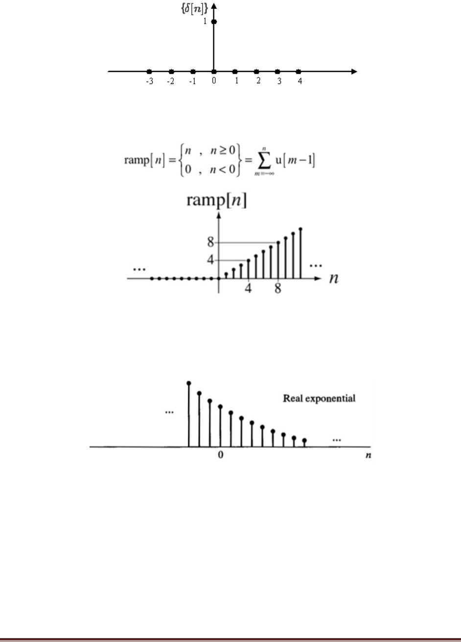
Unit impulse sequence :
δ(n)=1 n=0
0 n≠0
DIGITAL SIGNAL PROCESSING
Page 6
Unit Ramp sequence: It is defined as
Exponential sequence: it is a sequence of the form
x(n)=a
n
Sinusoidal signal:
It is represented as x(n)=Acos(w
o
n+Φ)

DIGITAL SIGNAL PROCESSING
Page 7
Complex exponential signal: It is represented as x(n)= a
n
e
j(won+Φ)
i.e x(n)= a
n
cos(w
o
n+Φ) +ja
n
sin(w
o
n+Φ)
1.2.2 Classification of Discrete time signals:
1. Energy and power signals.
2. Periodic and aperiodic signals.
3. Symmetric and asymmetric signals.
4. Causal and non causal signals.
5. Energy and power signals.
Energy and power signal: For a discrete time signal x(n) the energy E is given by
The average power of a Discrete time signal x(n) is

DIGITAL SIGNAL PROCESSING
Page 8
A signal is energy signal iff the total energy is finite.
Periodic and aperiodic signal:
A discrete time signal x(n) is said to be periodic with period N iff
x(N+n)= x(n) for all n
the smallest value of n for which the signal is periodic is called fundamental period.
If the above condition is valid then the signal is a periodic.
Fig: Periodic sequence fig: aperiodic sequence
Example: Show that the exponential sequence x(n)=e
jw0n
is periodic if w
0
/2π is rational
number.
Symmetric (even) and asymmetric (odd) signals:
A discrete time signal x(n) is said to be even it satisfies the condition
x(-n)=x(n) for all n

DIGITAL SIGNAL PROCESSING
Page 9
A discrete time signal x(n) is said to be odd it satisfies the condition
x(-n)=-x(n) for all n
this signals are represented as shown in fig.
Fig a.even signal b.odd signal
Causal and non causal signals: A signal x(n) is said to be causal if its value is zero for n<0,
otherwise the signal is non causal. A signal that is zero for all n 0 is called anti causal signal.
1.3 Linear Shift Invariant Systems:
A system is said to be linear shift(time) invariant if the characteristics of the
system does not change with time. In other words if the input sequence is shifted by k samples,
the generated output sequence is the original sequence shifted by k samples.

DIGITAL SIGNAL PROCESSING
Page 10
To test if any given system is time invariant first apply a sequence x(n) and find y(n). Now delay
the input sequence by k samples and find the output sequence.
Note: A linear time invariant system satisfies both linearity and time invariance property.
If the input to the system is unit impulse i.e x(n)=δ(n) then the output of the system is called
impulse response denoted by h(n).
h(n)=T[δ(n)]
for an LTI system if the input and impulse response are known then output y(n) is given by
y(n)=
the above equation represents output is the convolution sum of input sequence x(n) and impulse
response h(n) represented as
y(n)=x(n)*h(n)
1.4 STABILITY AND CAUSALITY
1.4.1 Stable and unstable systems
An LTI system is said to be stable if it produces bounded output sequence for every
bounded input sequence. If the input is bounded and output is unbounded then it is unstable
system. The necessary and sufficient condition for stability is

DIGITAL SIGNAL PROCESSING
Page 11
i.e., impulse response is stable if the impulse response is summable.
1.4.2 Causal System
Generally a causal system is a system whose output depends on only past and present
values of input. The output of an LTI system is given by
y(n)=
= y(n)=
+ y(n)=
=…………….h(-2)x(n+2)+h(-1)x(n+1)+h(0)x(n)+h(1)x(n-1)+…………..
As the causal system output does not depends on future inputs so neglect the terms then y(n)
reduces to
y(n)= h(0)x(n)+h(1)x(n-1)+…………..
=
i.e. h(k)=0 for k<0.
Therefore an LTI system is causal if and only if its impulse response is zero for negative values
of n.
1.5 LINEAR CONSTANT COEFFICIENT DIFFERENCE EQUATION.
There are different methods of analyzing the behavior or response of LTI system.
1. Direct solution of difference equation.
2. Discrete convolution.
3. Z transform
Direct Solution Of Difference Equation: the input and output relation of LTI system is
governed by constant coefficient difference equation of form
y(n)=
+
Mathematically the direct solution of above equation can be obtained to determine the response
of the system.
Discrete convolution: The output is convolution of input and impulse response.
y(n)=x(n)*h(n)

DIGITAL SIGNAL PROCESSING
Page 12
Z transform: The convolution property of z transform of the convolution of input and impulse
response is equa to the product of their individual z transforms.
i.e. Z[(n)*h(n)]=X(Z)H(Z)
but y(n)=x(n)*h(n)
so Z[y(n)]= X(Z)H(Z)
therefore y(n)=Z
-1
(X(Z)H(Z))
i.e the response y(n) of an LTI system is obtained by taking inverse Z transform of X(Z) and
H(Z). Conversely if the transfer function of the system is known then we can determine the
impulse response of system by taking inverse Z transform of transfer function.
i.e. h(n)=Z
-1
[H(Z)]=Z
-1
{Y(Z)/X(Z)}
1.6 FREQUENCY DOMAIN REPRESENTATION OF DISCRETE TIME SIGNALS and
SEQUENCES.
Fourier transform gives an effective representation of signals and systems in frequency domain.
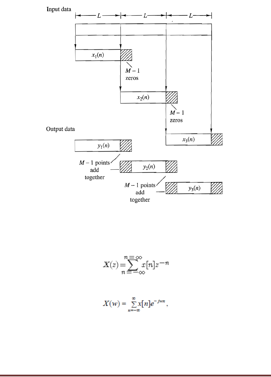
The Fourier transform of discrete time signal is given as
X(ω)=
e
-jwn
w is the frequency and it varies continuously from o to 2π. The magnitude of X(w) gives
frequency spectrum of x(n).
Y(w)=X(w)H(w)
H(w)= Y(w) / X(w)
H(w) is system function and h(n)=IFT[H(w)]
Discrete Time Fourier series:
Consider a periodic sequence x(n) with period N and this is expressed in discrete fourier series as
x(n)=
e
j2πnk/N
the values of C
k
k=0,1,2,3…………….N-1 are called discrete spectra of x(n). Each C
k
appears at
frequency w
k
=2πk/N.
Discrete Time Fourier Transform:
DFT is given by X (e
jw
) =
e
-jwn

DIGITAL SIGNAL PROCESSING
Page 13
Where X (e
jw
) is called DTFT of x(n)
x(n) is called IDTFT of X (e
jw
)
a sufficient condition for the existence of DTFT for a periodic sequence x(n) is
i.e sequence is absolutely summable.
1.7 Properties of DTFT
1.8 APPLICATIONS OF Z-TRANSFORMS:
The z-transform is a powerful mathematical tool used for the analysis of linear-time-
invariant discrete systems in frequency domain.
The z-transform has imaginary and real parts like fourier tansform .A plot of imaginary
part Vs real part is called Z-plane .This is also called complex Z-plane.
The poles and zeros of discrete LTI systems are plotted in the complex Z-plane. The
stability of LTI systems can also be determined from pole-zero plot.
DEFINATION OF Z-TRANSFORM AND REGION OF CONVERGENCE:
The Z-transform of a discrete time signal x(n) is denoted by X(Z)
Z-transform:

DIGITAL SIGNAL PROCESSING
Page 14
‘Z’ is the complex variable
X(Z) = Z[x(n)]
x(n) Z X(Z)
This Z-transform is also called as bilateral or two sided Z-transform
1.9 REGION OF CONVERGENCE:
Region of Convergence is the range of complex variable Z in the Z-plane. The Z-transformation
of the signal is finite or convergent. So, ROC represents those set of values of Z, for which X(Z)
has a finite value.
Z-transform is an “infinite series” (infinite power series) is not convergent for all values of Z
always.
PROPERTIES OF ROC
1.ROC does not include any pole.
2.For right-sided signal,ROC will be outside the circle in Z-plane.
3.For left sided signal,ROC will be inside the circle in Z-plane.
4.For stability,ROC includes unit circle in Z-plane.
5.For Both sided signal,ROC is a ring in Z-plane.
6.For finite-duration signal,ROC is entire Z-plane.
The Z-transform is uniquely characterized by:
1.Expression of X(Z)
2.ROC of X(Z)

DIGITAL SIGNAL PROCESSING
Page 15
Example: Determine Z-transform and ROC of the signal x(n)=a
n
u(n)+b
n
(-n-1)
Solution:
Given x(n)=a
n
u(n)+b
n
(-n-1)
X(Z ) =
z
-n
+
z
-n
=
+
z)
n
=
+
z)
n -
1]
=
+
=
+
-1
=
<1 +
<1
a
b

DIGITAL SIGNAL PROCESSING
Page 16
ROC
:
>
&
>
>
X(Z)
+
- 1
=
+
Example: Determine Z-transform of the signal
1.10 SOLUTION OF DIFFERENCE EQUATIONS OF DIGITAL FILTERS
The N
th
order system or digital filters are described by a general form of linear constant
coefficient difference equation as
y(n-k) =
x(n-k)
Where y(n) is output ,x(n) is input and
,
are linear constant coefficients
Taking
= 1, y(n) = -
y(n-k) +
x(n-k)
RESPONSE OF SYSTEM WITH ZERO INITIAL CONDITIONS:
System function H(Z) of system ,represent H(Z) as a ratio of two polynomials B(Z)/A(Z),
Where B(Z) is the numerator that contains zeros of H(Z) and
A(Z) is the denominator polynomial that determines poles of H(Z) input signal x(n) has a
rational z-transform X(Z).

DIGITAL SIGNAL PROCESSING
Page 17
ie,. X(Z) =
Z-transform of the output of system has the form
Y(Z)= H(Z) X(Z) =
Suppose that system contains simple poles P
1
, P
2
, P
3,…
P
N
and Z-transform of the input signal
contains poles q
1
, q
2
, q
3,…
q
L
, where P
k
≠ qm for all k = 1,2,…N and m=1,2,…L.
The partial fraction expansions of Y(Z) yields as,
Y(Z) =
+
Inverse transform as y(n) =
)
n
u(n) +
(
)
n
u(n)
P
k
:
Function of poles (P
k
) of system is called natural response.
q
k
: of the input signal is called forced response of the system.
At initial conditions are zero the response y(n) is called zero state response
yzs (n) = y
n
(n) + y
f
(n)

DIGITAL SIGNAL PROCESSING
Page 18
Example: Solve the following difference equation using Z-transform method
1.11 STABILITY CRITERION:
A necessary and sufficient condition for linear time invariant system to be BIBO
stable is
˂ ∞
In turn, this condition implies that H(Z) most contain the unit circle within its ROC
Since H(Z) =
Take modulus on both sides
≤
When its evaluated on the unit circle
= 1

DIGITAL SIGNAL PROCESSING
Page 19
≤
Hence if the system is BIBO stable, the unit circle is constrained in the ROC of H(Z).
This can also be stated like “A linear time-invariant system is BIBO stable if and only if the
ROC of the system function includes the unit circle.
=
, k=1,2,…M
Unit sample response h(n) =
(n)
Where
(n) =
(
)
n
u(n)
For the system to be stable,
Each component of the sequence
(n) must satisfy the condition
˂ ∞
=
∞
n
|
=
∞
n
|
For the above system to be finite ,the magnitude of each term must be less than unity , ie,.. each
|
| ˂ 1, where
is a pole ie,.. |Z| <1.So , all poles of the system must lie inside the unit circle,
for the system to be stable.
1.12 SCHUR-COHN STABILITY TEST:
When the denominator polynomial of a transfer function of the system is large and which
cannot be factorized, it is not possible to find the poles of the system .Consequently we cannot
decide whether the system is stable or not. In such cases stability can be decided by using Schur-
Cohn Stability Test.
Let us consider transfer function of a system ,whose stability to be decided ,
H(Z) =
consider only the denominator polynomial, here order of the
denominator polynomial is 2 .So denote the polynomial as D
2
(Z) =
.
Let k
2
= -
and k
2
=
,If k
2
is greater than or equal to 1,system is unstable .
If k
2
is less than 1,then find k
1
by forming reverse polynomial R
2
(Z) from which D
1
(Z) .
Can be found by using D
1
(Z) = D
2
(Z)- k
2
R
2
(Z)
1- k
2
2

DIGITAL SIGNAL PROCESSING
Page 20
Here | k
2
| < 1 So form the reverse polynomial R
2
(Z) =
Therefore, D
1
(Z) = D
2
(Z)- k
2
R
2
(Z)
1- k
2
2
On applying in the above formulae D
1
(Z) = 1-
; k
1= -
; |k
1
|
Here |k
1
| ˃ 1 ,so the system is unstable. If D
N
(Z) is given from R
N
(Z) use recursive equation
D
N-1
(Z) = D
N
(Z)- k
N
R
N
(Z) , to get k
N-1…,….
k
1
1- k
N
2
If anyone of k
N-1,…….
k
1
is greater than 1,stop calculating remaining K values and decide system as
unstable.
Example: Find the stability of the following transfer function H(Z) =
Solution: given H(Z) =
=
Since k
4
= 6 ; greater than 1 ; System unstable.
1.13FREQUENCY RESPONSE OF STABLE SYSTEM:
Discrete time Fourier transform and Z-transform s are used to obtain frequency response
of discrete time systems. If we set z = e
jωt
ie,.. evaluate z-transform around unit circle ,we get
the Fourier transform of the system with sampling time period,T.
H(e
jωt
) =H(ω) =
H(ω) is the frequency response of the system ,Its modulus gives the magnitude response and its
phase is the phase response
Magnitude/Phase Transfer Function using Fourier Transform:

DIGITAL SIGNAL PROCESSING
Page 21
Example: Calculate the frequency response for the LTI system representation
y(n) +
y(n-1)=x(n)-x(n-1)

DIGITAL SIGNAL PROCESSING
Page 22
Solution: Given y(n) +
y(n-1)=x(n)-x(n-1)
Taking Fourier transform on both sides
Y(e
jω
) +
e-
jω
Y(e
jω
) =X(e
jω
) - e-
jω
X(e
jω
)
Y(e
jω
) [1+
e-
jω
] = X(e
jω
) (1- e-
jω
)
H(e
jω
) =
=
|H
| =
=
1/2
Phase Response :
=
-
Ω
0
|H
|
0
0.4
0.6
0.8
0.5ᴨ
0.49ᴨ
0.42ᴨ
0.3ᴨ
|H
|
1.14 REALIZATION OF DIGITAL FILTERS :
A digital filter transfer function can be realized in a variety of ways .There are two types 0f
realization 1. Recursive 2. Non Recursive
For recursive realization the current output y(n) is a function of past outputs ,past and
present inputs. This form corresponds to an Infinite Impulse Response (IIR) digital filter. For a

DIGITAL SIGNAL PROCESSING
Page 23
Non recursive realization current output sample y(n) is a function of only past and present inputs.
This form corresponds to a Finite Impulse Response (FIR) digital filter.
IIR filter can be realized in many forms. They are :
1. Direct Form-I realization
2. Direct Form-II (Canonic) realization
3. Cascade Form
4. Parallel Form.
1.Direct Form-I realization :

DIGITAL SIGNAL PROCESSING
Page 24
1.14.1DIRECT FORM –II REALIZATION:

DIGITAL SIGNAL PROCESSING
Page 25
1.14.2 CASCADE FORM REALIZATION:
1.14.3 PARALLEL FORM REALIZATION:

DIGITAL SIGNAL PROCESSING
Page 26
Example:
Example: Obtain direct form I for the system described

DIGITAL SIGNAL PROCESSING
Page 27
EXAMPLE:

DIGITAL SIGNAL PROCESSING
Page 28

DIGITAL SIGNAL PROCESSING
Page 29
EXAMPLE:

DIGITAL SIGNAL PROCESSING
Page 30

DIGITAL SIGNAL PROCESSING
Page 31

DIGITAL SIGNAL PROCESSING
Page 32
UNIT 2
DISCRETE FOURIER SERIES
2.1 DFS REPRESENTATION OF PERIODIC SEQUENCE:
Consider a sequence x
p
(n) with a period of N samples so that x
p
(n)=x
p
(n+lN).since x
p
(n) is a
periodic ,it can be represented as a weighted sum of complex exponentials whose frequencies are
integer multiples of fundamental frequency.
These periodic complex exponentials are of the form
Any periodic sequence x(n) can be written as
2.2 PROPERTIES OF DISCRETE FOURIER SERIES:
1.LINEARITY OF DFS:
2. SHIFT OF A SEQUENCE:

DIGITAL SIGNAL PROCESSING
Page 33
3.COMPLEX CONJUGATION OF A PERIODIC SEQUENCE:
4.TIME REVERSAL:

DIGITAL SIGNAL PROCESSING
Page 34
5.TIME SCALING:
6.DIFFERENCE:
7.ACCUMULATION:

DIGITAL SIGNAL PROCESSING
Page 35
Example: Determine the spectra of the signals
2.3 DISCRETE FOURIER TRANSFORM:
The DFT of a finite duration sequence x(n) is obtained by sampling the fourier transform
X(e
jw
) at N equally spaced points over the interval 0≤w≤2π with a spacing of 2π/N.The DFT is
denoted by X(K),and is given by
For convenience
With this notation DFT analysis and synthesis equation is given by

DIGITAL SIGNAL PROCESSING
Page 36
2.4 SAMPLING OF THE FOURIER TRANSFORM:
The DFT values X(K) can be considered as samples of X(e
jw
).
2.5 PROPERTIES OF DFT:
1.LINEARITY:
2.CIRCULAR SHIFT OF A SEQUENCE:

DIGITAL SIGNAL PROCESSING
Page 37
3.SHIFT PROPERTY OF A DFT:
4.DUALITY:
5.SYMMETRY PROPERTIES:
6.CIRCULAR CONVOLUTION:

DIGITAL SIGNAL PROCESSING
Page 38
2.6 LINEAR CONVOLUTION USING DFT:
If we have sequence x(n) of length L and a sequence y(n) of length M, the sequence z(n)
obtained by linear convolution has length (L+M-1).This can be seen from the definition

DIGITAL SIGNAL PROCESSING
Page 39
Example : Find the DFT of given sequence

DIGITAL SIGNAL PROCESSING
Page 40
Example :

DIGITAL SIGNAL PROCESSING
Page 41

DIGITAL SIGNAL PROCESSING
Page 42
DIGITAL SIGNAL PROCESSING
Page 43
2.7 RELATION BETWEEN Z-TRANSFORM AND DTFT:
The Z-transform of a signal x(n) is given by
The DTFT of a signal x(n) is given by
Relation is given by
Z=e
jw

DIGITAL SIGNAL PROCESSING
Page 44
2.8 RELATION BETWEEN DTFT AND DFT:
The DTFT of a signal x(n) is given by
The DFT of a signal x(n) is given by
2.9 FAST FOURIER TRANSFORM
COMPUTATIONAL COMPLEXITY OF DFT AND FFT:
DFT:
No.of complex multiplications=N
2
No.of complex additions=N(N-1)
FFT:
No.of complex multiplications=Nlog
2
N
No.of complex additions=N/2log
2
N
INTRODUCTION:
In this section we present several methods for computing the DFT efficiently. In view of the
importance of the DFT in various digital signal processing applications, such as linear filtering,
correlation analysis, and spectrum analysis, its efficient computation is a topic that has received
considerable attention by many mathematicians, engineers, and applied scientists.
From this point, we change the notation that X(k), instead of y(k) in previous sections,
represents the Fourier coefficients of x(n).

DIGITAL SIGNAL PROCESSING
Page 45
Basically, the computational problem for the DFT is to compute the sequence {X(k)}
of N complex-valued numbers given another sequence of data {x(n)} of length N, according to
the formula
In general, the data sequence x(n) is also assumed to be complex valued. Similarly, The IDFT
becomes
Since DFT and IDFT involve basically the same type of computations, our discussion of
efficient computational algorithms for the DFT applies as well to the efficient computation of the
IDFT.
We observe that for each value of k, direct computation of X(k) involves N complex
multiplications (4N real multiplications) and N-1 complex additions (4N-2 real additions).
Consequently, to compute all N values of the DFT requires N
2
complex multiplications and N
2
-
N complex additions.
Direct computation of the DFT is basically inefficient primarily because it does not exploit the
symmetry and periodicity properties of the phase factor W
N
. In particular, these two properties
are :
The computationally efficient algorithms described in this sectio, known collectively as fast
Fourier transform (FFT) algorithms, exploit these two basic properties of the phase factor.
2.10 RADIX-2 DIT-FFT ALGORITHM:
Let us consider the computation of the N = 2
v
point DFT by the divide-and conquer approach.
We split the N-point data sequence into two N/2-point data sequences f
1
(n) and f
2
(n),
corresponding to the even-numbered and odd-numbered samples of x(n), respectively, that is,

DIGITAL SIGNAL PROCESSING
Page 46
Thus f
1
(n) and f
2
(n) are obtained by decimating x(n) by a factor of 2, and hence the resulting
FFT algorithm is called a decimation-in-time algorithm.
Now the N-point DFT can be expressed in terms of the DFT's of the decimated sequences as
follows:
But W
N
2
= W
N/2
. With this substitution, the equation can be expressed as
where F
1
(k) and F
2
(k) are the N/2-point DFTs of the sequences f
1
(m) and f
2
(m), respectively.
Since F
1
(k) and F
2
(k) are periodic, with period N/2, we have F
1
(k+N/2) = F
1
(k) and F
2
(k+N/2)
= F
2
(k). In addition, the factor W
N
k+N/2
= -W
N
k
. Hence the equation may be expressed as
We observe that the direct computation of F
1
(k) requires (N/2)
2
complex multiplications. The
same applies to the computation of F
2
(k). Furthermore, there are N/2 additional complex
multiplications required to compute W
N
k
F
2
(k). Hence the computation of X(k) requires
2(N/2)
2
+ N/2 = N
2
/2 + N/2 complex multiplications. This first step results in a reduction of the
number of multiplications from N
2
to N
2
/2 + N/2, which is about a factor of 2 for N large.

DIGITAL SIGNAL PROCESSING
Page 47
By computing N/4-point DFTs, we would obtain the N/2-point DFTs F
1
(k) and F
2
(k) from the
relations
The decimation of the data sequence can be repeated again and again until the resulting
sequences are reduced to one-point sequences. For N = 2
v
, this decimation can be performed v =
log
2
N times. Thus the total number of complex multiplications is reduced to (N/2)log
2
N. The
number of complex additions is Nlog
2
N.

DIGITAL SIGNAL PROCESSING
Page 48
FIG.8-point fft using four 2-point Dfts

DIGITAL SIGNAL PROCESSING
Page 49
Fig.Butterfly diagram for DIT-FFT Algorithm
An important observation is concerned with the order of the input data sequence after it is
decimated (v-1) times. For example, if we consider the case where N = 8, we know that the first
decimation yeilds the sequence x(0), x(2), x(4), x(6), x(1), x(3), x(5), x(7), and the second
decimation results in the sequence x(0), x(4), x(2), x(6), x(1), x(5), x(3), x(7). This shuffling of the
input data sequence has a well-defined order as can be ascertained from observing Figure
TC.3.5, which illustrates the decimation of the eight-point sequence.

DIGITAL SIGNAL PROCESSING
Page 50
Example :Find the FFT of a given sequence x(n)={1,2,3,4}by using DIT-FFT Algorithm?
Example : Find the IFFT of a given sequence x(k)={10,-2+2j,-2,-2-2j}by using DIT-IFFT
Algorithm?

DIGITAL SIGNAL PROCESSING
Page 51
2.11 RADIX-2 DIF-FFT ALGORITHM:
Another important radix-2 FFT algorithm, called the decimation-in-frequency algorithm, is
obtained by using the divide-and-conquer approach. To derive the algorithm, we begin by
splitting the DFT formula into two summations, one of which involves the sum over the first N/2
data points and the second sum involves the last N/2 data points. Thus we obtain
Now, let us split (decimate) X(k) into the even- and odd-numbered samples. Thus we obtain
where we have used the fact that W
N
2
= W
N/2
The computational procedure above can be repeated through decimation of the N/2-point
DFTs X(2k) and X(2k+1). The entire process involves v = log
2
N stages of decimation, where
each stage involves N/2 butterflies of the type shown in Figure TC.3.7. Consequently, the
computation of the N-point DFT via the decimation-in-frequency FFT requires (N/2)log
2
N
complex multiplications and Nlog
2
N complex additions, just as in the decimation-in-time
algorithm. For illustrative purposes, the eight-point decimation-in-frequency algorithm is given
in Figure.

DIGITAL SIGNAL PROCESSING
Page 52
FIG.8-point FFT using two 4-point DFT
Fig. Butterfly diagram for DIF-FFT Algorithm

DIGITAL SIGNAL PROCESSING
Page 53
Example :Find the FFT of a given sequence x(n)={1,2,3,4}by using DIF-FFT Algorithm?
Example :Find the IFFT of a given sequence x(k)={10,-2+2j,-2,-2-2j}by using DIF-IFFT
Algorithm?

DIGITAL SIGNAL PROCESSING
Page 54
Unit 3
IIR FILTERS
ANALOG FILTER APPROXIMATIONS:
Basically a digital filter is a linear time invariant discrete time system. The terms infinite
impulse response (IIR) and finite impulse response (FIR) are used to distinguish filter types. The
FIR filters are of non-recursive type, where the present output sample depends on present and
previous input samples. IIR are of non-recursive type where the present output depends on
previous and past input samples and output samples.
FREQUENCY SELECTIVE FILTERS:
A filter is one which rejects unwanted frequencies from the input and allows the desired
frequencies to obtain the required shape of output signal. The range of frequencies that are
passed through the filter is called pass band and those frequencies that are blocked are called stop
band. The filters are of different types :
1.Low Pass Filter 2.High Pass Filter 3.Band Pass Filter 4.Band Reject Filter
DESIGN OF DIGITAL FILTERS FROM ANALOG FILTERS:
For the given specifications of a digital filter the derivation of digital filter transfer
function requires three steps:
1. Map the desired digital filter specifications into equivalent analog filter.
2. Obtain the analog transfer function.
3. Transfer the analog transfer function to equivalent digital filter transfer function.
Fig (a): Magnitude response of analog LPF Fig (b): Magnitude response of digital LPF

DIGITAL SIGNAL PROCESSING
Page 55
Where,
= Pass band frequency in radians
= Stop band frequency in radians
= 3dB cutoff frequency in radians
ε = Parameter specifying allowable Pass band
λ = Parameter specifying allowable Stop band
Fig : Alternate specification of magnitude response of LPF
= Pass band error tolerance
= Stop band error tolerance
The relation between parameters are
ε = 2
and λ =
ANALOG LOW PASS FILTER DESIGN:
The general form of analog filter transfer function is
H(s) =
=
Where H(s) is the Laplace Transform of impulse response of h(t) and N≥M must be satisfied.
For a stable analog filter the poles of H(s) lies in the left half of the s-plane.
The two types of analog filters we design are: 1.Butterworth Filter 2.Chebyshev Filter.

DIGITAL SIGNAL PROCESSING
Page 56
ANALOG LOW PASS BUTTERWORTH FILTER:
The squared magnitude response of butterworth low pass filter is given by
Where, N= Order of the filter
Ωc = Cutoff frequency
The magnitude response decrease monotonically as shown in figure and the maximum response
is unity at Ω=0 ie,.. as the N increases the response approaches ideal low pass characteristics.
Fig: Low Pass butterworth magnitude response.
We can get magnitude square function of normalized butterworth filter(1 rad/sec cut off
frequency) as
|H(jΩ)|
2
=
N=1,2,3…
For transfer function of stable filter substitute Ω=s/j in above eqn.
|H(jΩ)|
2
=|H(Ω)|
2
=H(-s
2
)=H(jΩ)H(-jΩ)=
H(s)H(-s)=
=
Equating denominator to zero, poles are obtained
i.e
=0
for N odd, the above equation reduces to s
2N
= 1=e
j2πk

DIGITAL SIGNAL PROCESSING
Page 57
now the roots can be found as s
k
= e
jπk/N
k=1,2,3,………2N
for N even, the above equation reduces to s
2N
= -1=e
j(2k-1)π
which gives s
k
= e
j(2k-1)π/2N
k=1,2,3….
Note: The poles which lie in the left half of the s plane, the same can be found using the formula
s
k
=e
jφ
k
where
φ
k
=
+
k=1,2,3………..N
LIST OF BUTTERWORTH POLYNOMIALS:
The unnormalised poles are given by s
k
’=Ω
c
s
k
.
The transfer function of butterworth filter can be obtained by substituting s s/Ω
c
ORDER OF FILTER
The magnitude function is given as
|H(jΩ)|
2
=
Taking log on both sides
20 log |H(jΩ)|=10log1-10log[
at pass band frequency the attenuation is equal to α
p

DIGITAL SIGNAL PROCESSING
Page 58
20 log |H(jΩp)|= - α
p
= -10log[
α
p
=10log[
0.1 α
p
=log[
By taking antilog on both sides
ε=(10
0.1
α
p
-1)
1/2
at stop band frequency the minimum attenuation is equal to α
s
20 log |H(jΩ)|=10log1-10log[
20 log |H(jΩp)|= - α
s
= -10log[
0.1α
s
=log[
=
Taking log on both sides
N =
Round off N to next higher integer.
N ≥
N ≥
where λ
2
=
ε
2
=
]
For simplicity A=
and k=
Ω
Ω
the transition ratio
Therefore, the order of the low pass butterworth analog filter N=

DIGITAL SIGNAL PROCESSING
Page 59
ANALOG LOW PASS CHEBYSHEV FILTER
The magnitude squared response of the analog lowpassType I Chebyshevfilter of Nth order is
given by:
|H(W)|2= 1/[1 + e2TN2(W/Wp)].
where TN(W) is the Chebyshev polynomial of order N:
TN(W) = cos(Ncos-1W),|W| ≤1,
= cosh(Ncosh-1W),|W| > 1.
The polynomial can be derived via a recurrence relation given by
Tr(W) = 2WTr-1(W) –Tr-2(W),r ≥2, with T0(W) = 1 and T1(W) = W.
The magnitude squared response of the analog lowpassType II or inverse Chebyshevfilter of Nth
order is given by:
|H(W)|2= 1/[1 + e2{TN(Ws/Wp)/ TN(Ws/W)}2].
Equiripple in the passband and monotonic in the stopband.
Or equiripple in the stopband and monotonic in the passband.

DIGITAL SIGNAL PROCESSING
Page 60

DIGITAL SIGNAL PROCESSING
Page 61
DESIGN OF IIR FILTER FROM ANALOG FILTERS
1. IMPULSE INVARIANCE
2. STEP INVARIANT
3. BILINEAR TRANSFORMATION
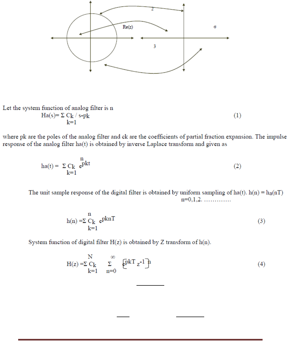
Impulse Invariance Method is simplest method used for designing IIR Filters. Important
Features of this Method are
1. In impulse variance method, Analog filters are converted into digital filter just by replacing
unit sample response of the digital filter by the sampled version of impulse response of analog
filter. Sampled signal is obtained by putting t=nT hence h(n) = ha(nT) n=0,1,2. ………….
where h(n) is the unit sample response of digital filter and T is sampling interval.
2. But the main disadvantage of this method is that it does not correspond to simple algebraic
mapping of S plane to the Z plane. Thus the mapping from analog frequency to digital frequency

DIGITAL SIGNAL PROCESSING
Page 62
is many to one. The segments (2k-1)Π/T ≤ Ω ≤ (2k+1) Π/T of jΩ axis are all mapped on the unit
circle Π≤ω≤Π. This takes place because of sampling.
3. Frequency aliasing is second disadvantage in this method. Because of frequency aliasing, the
frequency response of the resulting digital filter will not be identical to the original analog
frequency response.
4. Because of these factors, its application is limited to design low frequency filters like LPF or
a limited class of band pass filters.
RELATIONSHIP BETWEEN Z PLANE AND S PLANE
In impulse invariant method the IIR filter is designed such that unit impulse response h(n)
of digital filter is the sampled version of the impulse response of analog filter.
The Z transform of IIR is given by
H(Z)=
H(Z)/z=e
sT
=
Z is represented as re
jω
in polar form and relationship between Z plane and S plane is given as
Z=e
ST
where s= σ + j Ω.
Z= e
ST
(Relationship Between Z plane and S plane)
Z= e
(σ + j Ω) T
= e
σ T
. e
j Ω T
Comparing Z value with the polar form we have.
r= e
σ T
and ω = Ω T
Here we have three condition
1) If σ = 0 then r=1
2) If σ < 0 then 0 < r < 1
3) If σ > 0 then r> 1
Thus
1) Left side of s-plane is mapped inside the unit circle.
2) Right side of s-plane is mapped outside the unit circle.
3) jΩ axis is in s-plane is mapped on the unit circle.
Im(z)
)
DIGITAL SIGNAL PROCESSING
Page 63
Fig: Impulse invariant pole mapping
=
Using the standard relation and comparing equ 1 and 4
If H
a
(s)=
then H(z)=
S plane

DIGITAL SIGNAL PROCESSING
Page 64
Steps to design Digital IIR Filter using impulse invariant technique:
1. For the given specifications, find Ha(s), transfer function of an analog filter.
2. Select the sampling rate of the digital filter .
3. Express the analog filter transfer function as the sum of single pole filters.
Ha(s)=
4. Compute the z transform of the digital filter by using the formula.
H(z)=
Example:
STEP INVARIANT METHOD:
The step response y(t) is defined as the output of a LTI system due to a unit step input
signal x(t)=u(t).Then
X(s)=
and Y(s)= X(s)H(s)=
H(s).
We know that a digital filter is equivalent to an analog filter in the sense of time domain
invariance, if equivalent input yield equivalent outputs.
Therefore the sampled input to digital filter is x(nT)=x(n)=u(n)Then
X(z)=
and y(n)=y(nT).
The transfer function of the digital filter is given by
H(z)= Y(z)/X(z)=(1-z
-1
)Y(z).

DIGITAL SIGNAL PROCESSING
Page 65
BILINEAR TRANSFORMATION METHOD:

DIGITAL SIGNAL PROCESSING
Page 66
Ω=
Up on simplification, we get
WARPING EFFECT
Let Ω and ω represents the frequency variables in the analog filter and the derived digital
filter resp.
Ω=
tan
For small value of ω
Ω=
=
ω=ΩT
For low frequencies the relation between ω and Ω are linear, as a result the digital filter have the
same amplitude response as analog filter. For high frequencies however the relation between
ω and Ω becomes nonlinear and distortion is introduced in the frequency scale of digital filter to
that of analog filter. This is known as warping effect.
Fig: Relationship between ω and Ω

DIGITAL SIGNAL PROCESSING
Page 67
The influence of the warping effect on amplitude response is shown in figure below. The analog
filter with a number of pass bands centered at regular intervals. The derived digital filter will
have same number of pass bands. But the centre frequencies and bandwidth of higher frequency
pass band will tend to reduce disproportionately.
Fig : Effect on magnitude response due to warping effect
The influence of warping effect on the phase response is as shown below ,Considering an analog
filter with linear phase response, the phase response of derived digital filter will be non linear.
ω
ΩT
Ω
∟H(jΩ)
∟H(e
jω
)

DIGITAL SIGNAL PROCESSING
Page 68
Prewarping
The prewarping effect can be eliminated by prewarping the analog filter. This can be done
by finding prewarping analog frequencies using the formula
Ω=
tan
Therefore we have Ωp=
tan
And Ωs=
tan
STEPS TO DESIGN DIGITAL FILTER USING BILINEAR TRANSFORM
TECHNIQUE:
1. From the given specifications, find prewarping analog frequencies using formula
Ω=
tan
.
2. Using the analog frequencies find H(s) of the analog filter.
3. Select the sampling rate of the digital filter, call it T sec/sample.
4. Substitute z =
into the transfer function.
SPECTRAL TRANSFORMATIONS:
IN ANALOG DOMAIN : A analog low pass filter can be converted into a analog High Pass,
Band Stop, Band Pass or another Low Pass digital filter as given below
Low Pass to Low Pass:
s
Low Pass to High Pass:
s
Low Pass to Band Pass:
s
Low Pass to Band Stop:
s

DIGITAL SIGNAL PROCESSING
Page 69
IN DIGITAL DOMAIN:
A digital low pass filter can be converted into a digital High Pass, Band Stop, Band Pass
or another Low Pass digital filter as given below
Low Pass to Low Pass:
Z
-1
Where α =
ω
p
=
Pass band frequency of low pass
filter
ω
p
’ = Pass band frequency of new
filter
Low Pass to High Pass:
Z
-1 ---
Where α =
ω
p
=
Pass band frequency of low pass
filter
ω
p
’ = Pass band frequency of high pass
filter
Low Pass to Band Pass:
Z
-1 ---
Where α=
and k=
[tan
/2)]
= Upper cutoff frequency
= Lower cutoff frequency
Low Pass to Band Stop:
Z
-1 ---
Where α=
and k=
[tan
/2)]
= Upper cutoff frequency
= Lower cutoff frequency

DIGITAL SIGNAL PROCESSING
Page 70
PROBLEMS
1.

DIGITAL SIGNAL PROCESSING
Page 71

DIGITAL SIGNAL PROCESSING
Page 72
2.
Solution:

DIGITAL SIGNAL PROCESSING
Page 73
UNIT 4
FIR FILTERS
4.1 INTRODUCTION
The FIR Filters can be easily designed to have perfectly linear Phase. These filters can be
realized recursively and Non-recursively. There is greater flexibility to control the Shape of their
Magnitude response. Errors due to round off noise are less severe in FIR Filters, mainly because
Feedback is not used.
4.2 FEATURES OF FIR FILTER:
1. FIR filter always provides linear phase response. This specifies that the signals in the pass
band will suffer no dispersion Hence when the user wants no phase distortion, then FIR
filters are preferable over IIR. Phase distortion always degrades the system performance. In
various applications like speech processing, data transmission over long distance FIR filters
are more preferable due to this characteristic.
2. FIR filters are most stable as compared with IIR filters due to its non feedback nature.
3. Quantization Noise can be made negligible in FIR filters. Due to this sharp cutoff
FIR filters can be easily designed.
4. Disadvantage of FIR filters is that they need higher ordered for similar magnitude response of
IIR filters.
4.3 FIR SYSTEM ARE ALWAYS STABLE. Why?
Proof: Difference equation of FIR filter of length M is given as
M-1
y(n)=Σ bk x(n–k)
k=0
And the coefficient bk are related to unit sample response as
H(n) = bn for 0 ≤ n ≤ M-1
= 0 otherwise.
We can expand this equation as
Y(n)= b0 x(n) + b1 x(n-1) + …….. + bM-1 x(n-M+1)
System is stable only if system produces bounded output for every bounded input. This is
stability definition for any system.
Here h(n)={b0, b1, b2, } of the FIR filter are stable. Thus y(n) is bounded if input x(n) is

DIGITAL SIGNAL PROCESSING
Page 74
bounded. This means FIR system produces bounded output for every bounded
input. Hence FIR systems are always stable.
4.4 SYMMETRIC AND ANTI-SYMMETRIC FIR FILTERS:
1. Unit sample response of FIR filters is symmetric if it satisfies following condition.
h(n)= h(M-1-n) n=0,1,2…………….M-1
2. Unit sample response of FIR filters is Anti-symmetric if it satisfies following condition
h(n)= -h(M-1-n) n=0,1,2…………….M-1
4.5 FIR FILTER DESIGN METHODS:
The various method used for FIR Filer design are as follows
1. Fourier Series method
2. Windowing Method
3. DFT method
4. Frequency sampling Method. (IFT Method)
GIBBS PHENOMENON:
Consider the ideal LPF frequency response as shown in Fig 1 with a
normalizing angular cut off frequency Ωc.
Impulse response of an ideal LPF is as shown in Fig 2.
1. In Fourier series method, limits of summation index is -∞ to ∞. But filter must have finite
terms.Hence limit of summation index change to -Q to Q where Q is some finite integer. But this
type of truncation may result in poor convergence of the series. Abrupt truncation of infinite

DIGITAL SIGNAL PROCESSING
Page 75
series is equivalent to multiplying infinite series with rectangular sequence. i.e at the point of
discontinuity some oscillation may be observed in resultant series.
2. Consider the example of LPF having desired frequency response Hd (ω) as shown in figure.
The oscillations or ringing takes place near band-edge of the filter.
3. This oscillation or ringing is generated because of side lobes in the frequency response
W(ω) of the window function. This oscillatory behavior is called "Gibbs Phenomenon”.
Truncated response and ringing effect is as shown in fig 3.
4.6 WINDOWING TECHNIQUE:
Windowing is the quickest method for designing an FIR filter. A windowing function simply
truncates the ideal impulse response to obtain a causal FIR approximation that is non causal and
infinitely long. Smoother window functions provide higher out-of band rejection in the filter
response.
However this smoothness comes at the cost of wider stopband transitions.Various windowing
method attempts to minimize the width of the main lobe (peak) of the frequency response. In
addition, it attempts to minimize the side lobes (ripple) of the frequency response.
Rectangular Window: Rectangular This is the most basic of windowing methods. It does not
require any operations because its values are either 1 or 0. It creates an abrupt discontinuity that
results in sharp roll-offs but large ripples.

DIGITAL SIGNAL PROCESSING
Page 76
Rectangular window is defined by the following equation.
Triangular Window: The computational simplicity of this window, a simple convolution of two
rectangle windows, and the lower sidelobes make it a viable alternative to the rectangular
window.
Kaiser Window: This windowing method is designed to generate a sharp central peak. It has
reduced side lobes and transition band is also narrow. Thus commonly used in FIR filter design.

DIGITAL SIGNAL PROCESSING
Page 77
Hamming Window: This windowing method generates a moderately sharp central peak. Its
ability to generate a maximally flat response makes it convenient for speech processing filtering.
Hanning Window: This windowing method generates a maximum flat filter design.

DIGITAL SIGNAL PROCESSING
Page 78
WINDOWING FUNCTIONS FOR
RECTANGULAR,HANNING,HAMMING,BLACKMAN WINDOWS
4.7 DESIGNING FILTER FROM POLE ZERO PLACEMENT:
Filters can be designed from its pole zero plot. Following two constraints should be
imposed while designing the filters.
1. All poles should be placed inside the unit circle on order for the filter to be stable. However
zeros can be placed anywhere in the z plane. FIR filters are all zero filters hence they are always
stable. IIR filters are stable only when all poles of the filter are inside unit circle.
2. All complex poles and zeros occur in complex conjugate pairs in order for the filter
coefficients to be real.

DIGITAL SIGNAL PROCESSING
Page 79
In the design of low pass filters, the poles should be placed near the unit circle at points
corresponding to low frequencies ( near ω=0)and zeros should be placed near or on unit circle at
points corresponding to high frequencies (near ω=Π). The opposite is true for high pass filters.
4.8 FREQUENCY SAMPLING METHOD FOR DESIGNING FIR DIGITAL FILTERS:

DIGITAL SIGNAL PROCESSING
Page 80

DIGITAL SIGNAL PROCESSING
Page 81
4.9 COMPARISON BETWEEN FIR AND IIR DIGITAL FILTERS:

DIGITAL SIGNAL PROCESSING
Page 82

DIGITAL SIGNAL PROCESSING
Page 83

DIGITAL SIGNAL PROCESSING
Page 84

DIGITAL SIGNAL PROCESSING
Page 85
PROBLEMS
solution:

DIGITAL SIGNAL PROCESSING
Page 86

DIGITAL SIGNAL PROCESSING
Page 87

DIGITAL SIGNAL PROCESSING
Page 88

DIGITAL SIGNAL PROCESSING
Page 89
UNIT-5
MULTIRATE SIGNAL PROCESSING
INTRODUCTION:
Multirate means "multiple sampling rates". A multirate DSP system uses multiple
sampling rates within the system. Whenever a signal at one rate has to be used by a system that
expects a different rate, the rate has to be increased or decreased, and some processing is required to
do so. Therefore "Multirate DSP" really refers to the art or science of changing sampling
Need of Multirate DSP:
The most immediate reason is when you need to pass data between two systems which
use incompatible sampling rates. For example, professional audio systems use 48 kHz rate, but
consumer CD players use 44.1 kHz; when audio professionals transfer their recorded music to
CDs, they need to do a rate conversion.But the most common reason is that multirate DSP can
greatly increase processing efficiency (even by orders of magnitude!), which reduces DSP
system cost. This makes the subject of multirate DSP vital to all professional DSP practitioners
Categories of Multirate: Multirate consists of:
1. Decimation: To decrease the sampling rate,
2. Interpolation: To increase the sampling rate,
3. Resampling:To combine decimation and interpolation in order to change the sampling
rate by a fractional value that can be expressed as a ratio. For example, to resample by a
factor of 1.5, you just interpolate by a factor of 3 then decimate by a factor of 2 (to
change the sampling rate by a factor of 3/2=1.5.)
APPLICATIONS:
1. Used in A/D and D/A converters.
2. Used to change the rate of a signal. When two devices that operate at different rates are to be
interconnected, it is necessary to use a rate changer between them.
3. In transmultiplexers
4. In speech processing to reduce the storage space or the transmitting rate of speech data.
5. Filter banks and wavelet transforms depend on multi rate methods.

DIGITAL SIGNAL PROCESSING
Page 90
DOWN SAMPLING:
The process of reducing a sampling rate by an integer factor is referredto as down
sampling of a data sequence. We also refer to down sampling as ''decimation''. To down
sample a data sequence x(n) by an integer factor of M, we use the following notation:
y(m) = x(mM)
Where y(m) is the down sampled sequence, Obtained by taking a sample from the data
sequence x(n) for every M samples (discarding M – 1 samples for every M samples). As an
example, if the original sequence with a sampling period T = 0.1 second (sampling rate = 10
samples per sec) is given by
Consider x(n):8 7 4 8 9 6 4 2 –2 –5 –7 –7 –6 –4 …
and we down sample the data sequence by a factor of 3, we obtain the down sampled sequence
as
y(m):8 8 4 –5 –6 … ,
with the resultant sampling period T = 3 × 0.1 = 0.3 second (the sampling rate now is 3.33
samples per second).
From the Nyquist sampling theorem, it is known that aliasing can occur in the down sampled
signal due to the reduced sampling rate. After down sampling by a factor of M, the new sampling
period becomes MT, and therefore the new sampling frequency is
f
sM
= 1/(MT) = f
s
/M,
where f
s
is the original sampling rate.
Hence, the folding frequency after down sampling becomes
f
sM
/2 = f
s
/(2M).

DIGITAL SIGNAL PROCESSING
Page 91
This tells us that after down sampling by a factor of M, the new folding frequency will be
decreased M times. If the signal to be down sampled has frequency components larger than the
new folding frequency, f > f
s
/(2M), aliasing noise will be introduced into the down sampled data.
To overcome this problem, it is required that the original signal x(n) be processed by a low pass
filter H(z) before down sampling, which should have a stop frequency edge at f
s
/(2M) (Hz). The
corresponding normalized stop frequency edge is then converted to be
Ω
stop
= 2π (f
s
/(2M)) T = π/M radians.
In this way, before down sampling, we can guarantee that the maximum frequency of the filtered
signal satisfies f
max
< f
s
/(2M),
such that no aliasing noise is introduced after down sampling. A general block diagram of
decimation is given in Figure, where the filtered output in terms of the z-transform can be written
as W(z) = H(z)X(z),
where X(z) is the z-transform of the sequence to be decimated,x(n), and H(z) is the lowpass filter
transfer function. After anti-aliasing filtering, the down sampled signal y(m) takes its value from
the filter output as: y(m) = w(mM).
The process of reducing the sampling rate by a factor of 3 is shown in Figure The corresponding
spectral plots for x(n),w(n), and y(m) in general are shown in Figure
Figure. Block diagram of the downsampling process with M = 3

DIGITAL SIGNAL PROCESSING
Page 92
Example:1: If x(n) = {1, -1, 2, 4, 0, 3, 2, 1, 5,….}
Then y(m)= x(mM) for M = 2 is
Y (m) = {1, 2, 0, 2, 5,….}
i.e if we left M-1 samples inbetween samples of x(n) to generate y(m).
Figure Spectrum after down sampling.

DIGITAL SIGNAL PROCESSING
Page 93
UP-SAMPLER :
Increasing a sampling rate is a process of upsampling by an integer factor of L. This process is
described as follows:
y(m) = x(m/L)
where n = 0, 1, 2, … , x(n) is the sequence to be up sampled by a factor of L, and y(m) is the up
sampled sequence. As an example, suppose that the data sequence is given as follows:
x(n) : 8 8 4 –5 –6 …
After up sampling the data sequence x(n) by a factor of 3 (adding L– 1 zeros for each sample),
we have the up sampled data sequence w(m) as:
w(m): 8 0 0 8 0 0 4 0 0 –5 0 0 –6 0 0 …
The next step is to smooth the up sampled data sequence via an interpolation filter. The process
is illustrated in Figure
Figure Block diagram for the upsampling process with L = 3.

DIGITAL SIGNAL PROCESSING
Page 94
Similar to the downsampling case, assuming that the data sequence has the current sampling
period of T, the Nyquist frequency is given by f
max
= f
s
/2. After upsampling by a factor ofL, the
new sampling period becomes T/L, thus the new sampling frequency is changed to be
f
sL
= Lf
s
. (12.10)
This indicates that after up sampling, the spectral replicas originally centered at f
s
, 2f
s
, … are
included in the frequency range from 0 Hz to the new Nyquist limit Lf
s
=2 Hz, as shown in
Figure. To remove those included spectral replicas, an interpolation filter with a stop frequency
edge of f
s
=2 in Hz must be attached, and the normalized stop frequency edge is given by
Ω
stop
= 2π (f
s
/2) × (T/L) = π/L radians.
Figure Spectra before and after upsampling.

DIGITAL SIGNAL PROCESSING
Page 95
After filtering via the interpolation filter, we will achieve the desired spectrum for y(n), as shown
in Figure 5.2.b. Note that since the interpolation is to remove the high-frequency images that are
aliased by the upsampling operation, it is essentially an anti-aliasing lowpass filter.
Example: If x(n) = {1, -1, 2, 4, 3, ,….}
Then y(m)= x(m/L) for L = 3 is
Y (m) = {1, 0, 0,-1,0, 0,2,0, 0, 4, 0, 0, 3, 0, 0,,….}
SAMPLE RATE CONVERSION:
In Decimation and Interpolation, sampling rate conversion is achieved by Integer Factor. When
sampling rate conversion requires by non integer factor, we need to perform sampling rate
conversion by rational factor I/D .
Perform Interpolation by a Factor I.
Filter the output of interpolator using a Low Pass (Anti Imaging Filter) with the
Bandwidth of π/I.
The output of Anti Imaging Filter is Passed through a another Low Pass Filter ( Anti
Aliasing Filter) to limit the bandwidth of signal to π/D.
Finally Signal Band limited to π/D is decimated by factor D.

DIGITAL SIGNAL PROCESSING
Page 96
The anti Imaging Filter and anti Aliasing Filter are operated at same sampling rate and
hence can be replaced by simple lowpass filter with cut off frequency,
W
c
= min[π/I, π/D]
It is Important to note that, in order to preserve the spectral characteristics of x(n), the
interpolation has to be performed first and decimation is to performed next
Example: Show that the upsampler and down sampler are time variant systems.
Consider a factor of L upsampler defined by
y(n) = x(n/L)
The o/p due to delayed i/p is
y( n, k) = x(n/L - k)
the delayed output is
y(n-k) = x[(n-k)/L]
y(n ,k ) y(n-k)
therefore up sampler is a time variant systems.
Similarly for down sampler
Y(n) = x(nM)
y(n,k) = x(nM-k)
y(n-k) = x(M(n-k))
y(n ,k ) y(n-k)
Therefore down sampler is a time variant systems.
FINITE WORD LENGTH EFFECTS
5.6 NUMBER REPRESENTATION:

DIGITAL SIGNAL PROCESSING
Page 97
In digital signal processing, (B +1)-bit fixed-point numbers are usually represented as two’s-
complementsigned fractions in the format bo b-ib-2 …… b-B
The number represented is then
where bo is the sign bit and the number range is —1 <X <1. The advantage of this representation
is that the product of two numbers in the range from — 1 to 1 is another number in the same
range. Floating-point numbers are represented as
where s is the sign bit, mis the mantissa, and cis the characteristic or exponent.To make the
representation of a number unique, the mantissa is normalized so that 0.5 <m <1.
Although floating-point numbers are always represented in the form of , the way in which this
representation is actually storedin a machine may differ. Since m >0.5, it is not necessary to store
the 2
-1
-weight bit of m, which is always set. Therefore, in practice numbers are usually stored as
where fis an unsigned fraction, 0 <f <0.5.
Most floating-point processors now use the IEEE Standard 754 32-bit floating point format for
storing numbers. According to this standard the exponent is stored as an unsigned integer pwhere
p = c +126
Therefore, a number is stored as
where s is the sign bit, fis a 23-b unsigned fraction in the range 0 <f <0.5, and p is an 8-b
unsigned integer in the range 0 <p <255. The total number of bits is 1 + 23 + 8 = 32. For
example, in IEEE format 3/4 is written (-1)
0
(0.5 + 0.25)2° so s =0, p =126, and f =0.25. The
value X =0 is a unique case and is represented by all bits zero (i.e., s = 0, f =0, and p =0).
Although the 2
-1
-weight mantissa bit is not actually stored, it does exist so the mantissa has 24 b
plus a sign bit.
5.7 FIXED-POINT QUANTIZATION ERRORS :
In fixed-point arithmetic, a multiply doubles the number of significant bits. For example, the
product of the two 5-b numbers 0.0011 and 0.1001 is the 10-b number 00.000 110 11. The extra
bit to the left of the decimal point can be discarded without introducing any error. However, the
DIGITAL SIGNAL PROCESSING
Page 98
least significant four of the remaining bits must ultimately be discarded by some form of
quantization so that the result can be stored to 5 b for use in other calculations. In the example
above this results in 0.0010 (quantization by rounding) or 0.0001(quantization by truncating).
When a sum of products calculation is performed, the quantization can be performed either after
each multiply or after all products have been summed with double length precision.
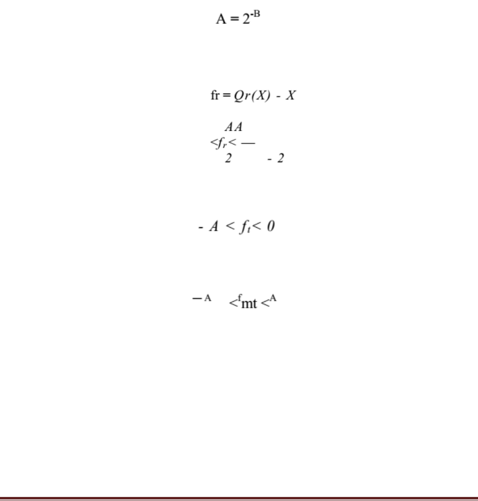
We will examine three types of fixed-point quantization—rounding, truncation, and magnitude
truncation. If X is an exact value, then the rounded value will be denoted Q
r
(X),the truncated
value Q
t
(X),and the magnitude truncated value Q
mt
(X).If the quantized value has Bbits to the
right of the decimal point, the quantization step size is
Since rounding selects the quantized value nearest the unquantized value, it gives a value which
is never more than ± A /2 awayfrom the exact value. If we denote the rounding error by
Truncation simply discards the low-order bits, giving a quantized value that is always less than
or equal to the exact value so
Magnitude truncation chooses the nearest quantized value that has a magnitude less than or equal
to the exact value so
The error resulting from quantization can be modeled as a random variable uniformly distributed
over the appropriate error range. Therefore, calculations with roundoff error can be considered
error-free calculations that have been corrupted by additive white noise. The meanof this noise
for rounding is
DIGITAL SIGNAL PROCESSING
Page 99
where E{}represents the operation of taking the expected value of a random variable. Similarly,
the variance of the noise for rounding is
Like wise for truncation,
And for magnitude truncation,
5.8 FLOATING-POINT QUANTIZATION ERRORS:
With floating-point arithmetic it is necessary to quantize after both multiplications and
additions. The addition quantization arises because, prior to addition, the mantissa of the smaller
number in the sum is shifted right until the exponent of both numbers is the same. In general, this
gives a sum mantissa that is too long and so must be quantized. We will assume that quantization
in floating-point arithmetic is performed by rounding. Because of the exponent in floating-point
arithmetic, it is the relative error that is important. The relative error is defined as
5.9 ROUNDOFF NOISE:
To determine the roundoff noise at the output of a digital filter we will assume that the noise due
to a quantization is stationary, white, and uncorrelated with the filter input, output, and internal

DIGITAL SIGNAL PROCESSING
Page 100
variables. This assumption isgood if the filter input changes from sample to sample in a
sufficiently complex manner. It is not valid for zero or constant inputs for which the effects of
rounding are analyzed from a limit cycle perspective.
To satisfy the assumption of a sufficiently complex input, roundoff noise in digital filters is often
calculated for the case of a zero-mean white noise filter input signal x(n)of variance a
1
. This
simplifies calculation of the output roundoff noise because expected values of the form
E{x(n)x(n — k)}are zero for k =0 and give a
2
when k =0. This approach to analysis has been
found to give estimates of the output roundoff noise thatare close to the noise actually observed
for other input signals.
Another assumption that will be made in calculating roundoff noise is that the product of two
quantization errors is zero. To justify this assumption, consider the case of a 16-b fixed-point
processor. In thiscase a quantization error is of the order 2
-15
, while the product of two
quantization errors is of the order 2
-30
, which is negligible by comparison.
If a linear system with impulse response g(n)is excited by white noise with mean m
x
and
variance a
2
, the output is noise of mean
And variance
Therefore, if g(n)is the impulse response from the point where a round off takes place to the filter
output, the contribution of that round off to the variance (mean square value) of the output round
off noise is given by with a
2
replaced with the variance of the round off. If there is more than
one source of round off error in the filter, it is assumed that the errors are uncorrelated so the
output noise variance is simply the sum of the contributions from each source.

DIGITAL SIGNAL PROCESSING
Page 101
5.10 LIMIT CYCLE OSCILLATIONS:
A limit cycle, sometimes referred to as a multiplier round off limit cycle, is a low level
oscillation that can exist in an otherwise stable filter as a result of the nonlinearity associated
with rounding (or truncating) internal filter calculations . Limit cycles require recursion to exist
and do not occur in non recursive FIR filters. As an example of a limit cycle, consider the
second-order filter realized by
where Qr{} represents quantization by rounding. This is stable filter with poles at 0.4375 ±
j0.6585. Consider the implementation of this filter with 4-b (3-b and a sign bit) two’s
complement fixed-point arithmetic, zero initial conditions (y(—1) = y(—2) = 0), and an input
sequence x(n) =|S(n), where S(n)is the unit impulse or unit sample. The following sequence is
obtained.
Notice that while the input is zero except for the first sample, the output oscillates with
amplitude 1/8 and period 6. Limit cycles are primarily of concern in fixed-point recursive filters.
As long as floating-point filters are realized as the parallel or cascade connection of first- and
second-order sub filters, limit cycles will generally not be a problem since limit cycles are
practically not observable in first and second-order systems implemented with 32-bit floating-
point arithmetic . It has been shown that such systems must have an extremely small margin of

DIGITAL SIGNAL PROCESSING
Page 102
stability for limit cycles to exist at anything other than underflow levels, which are at an
amplitude of less than . There are at least three ways of dealing with limit cycles when fixed-
point arithmetic is used. One is to determine a bound on the maximum limit cycle amplitude,
expressed as an integral number of quantization steps . It is then possible to choose a word length
that makes the limit cycle amplitude acceptably low. Alternately, limit cycles can be prevented
by randomly rounding calculations up or down. However, this approach is complicated to
implement. The third approach is to properly choose the filter realization structure and then
quantize the filter calculations using magnitude truncation . This approach has the disadvantage
of producing more round off noise than truncation or rounding .
5.11 OVERFLOW OSCILLATIONS:
With fixed-point arithmetic it is possible for filter calculations to overflow. This happens when
two numbers of the same sign add to give a value having magnitude greater than one. Since
numbers with magnitude greater than one are not representable, the result overflows. For
example, the two’s complement numbers 0.101 (5/8) and 0.100 (4/8) add togive 1.001 which is
the two’s complement representation of -7/8.
The overflow characteristic of two’s complement arithmetic can be represented as R{} where
An overflow oscillation, sometimes also referred to as an adder overflow limit cycle, is a high-
level oscillation that can exist in an otherwise stable fixed-point filter due to the gross
nonlinearity associated with the overflow of internal filter calculations .Like limit cycles,
overflow oscillations require recursion to exist and do not occur in non recursive FIR filters.
Overflow oscillations also do not occur with floating-point arithmetic due to the virtual
impossibility of overflow.
Quantization:
Total number of bits in x is reduced by using two methods namely Truncation and Rounding.
These are known as quantization Processes.
Input Quantization Error:
The Quantized signal are stored in a b bit register but for nearest values the same digital
equivalent may be represented. This is termed as Input Quantization Error.
Product Quantization Error:
The Multiplication of a b bit number with another b bit number results in a 2b bit number but it
should be stored in a b bit register. This is termed as Product Quantization Error.

DIGITAL SIGNAL PROCESSING
Page 103
Co-efficient Quantization Error:
The Analog to Digital mapping of signals due to the Analog Co-efficient Quantization results in
error due to the Fact that the stable poles marked at the edge of the jΩ axis may be marked as an
unstable pole in the digital domain.
Limit Cycle Oscillations:
If the input is made zero, the output should be made zero but there is an error occur due to the
quantization effect that the system oscillates at a certain band of values.
Overflow limit Cycle oscillations:
Overflow error occurs in addition due to the fact that the sum of two numbers may result in
overflow. To avoid overflow error saturation arithmetic is used.
Dead band:
The range of frequencies between which the system oscillates is termed as Deadband of the
Filter. It may have a fixed positive value or it may oscillate between a positive and negative
value.
Signal scaling:
The inputs of the summer is to be scaled first before execution of the addition operation to find
for any possibility of overflow to be occurredafter addition. The scaling factor s0is multiplied
with the inputs to avoid overflow.
