11472-02_Gerardi

SHANE M. SHERLUND

Board of Governors of the

Federal Reserve System

PAUL WILLEN

Federal Reserve Bank of Boston

Making Sense of the Subprime Crisis

ABSTRACT Should market participants have anticipated the large increase

in home foreclosures in 2007 and 2008? Most of these foreclosures stemmed

from mortgage loans originated in 2005 and 2006, raising suspicions that

lenders originated many extremely risky loans during this period. We show

that although these loans did carry extra risk factors, particularly increased

leverage, reduced underwriting standards alone cannot explain the dramatic

rise in foreclosures. We also investigate whether market participants under-

estimated the likelihood of a fall in home prices or the sensitivity of fore-

closures to falling prices. We show that given available data, they should

have understood that a signiﬁcant price drop would raise foreclosures sharply,

although loan-level (as opposed to ownership-level) models would have pre-

dicted a smaller rise than occurred. Analyst reports and other contemporary

discussions reveal that analysts generally understood that falling prices would

have disastrous consequences but assigned that outcome a low probability.

ad market participants anticipated the increase in defaults on sub-

prime mortgages originated in 2005 and 2006, the nature and extent

of the current ﬁnancial market disruptions would be very different. Ex

ante, investors in subprime mortgage-backed securities (MBSs) would

have demanded higher returns and greater capital cushions. As a result,

borrowers would not have found credit as cheap or as easy to obtain as it

became during the subprime credit boom of those years. Rating agencies

would have reacted similarly, rating a much smaller fraction of each deal

investment grade. As a result, the subsequent increase in foreclosures

would have been significantly smaller, with fewer attendant disruptions

in the housing market, and investors would not have suffered such out-

sized, and unexpected, losses. To make sense of the subprime crisis, one

needs to understand why, when accepting significant exposure to the

KRISTOPHER GERARDI

Federal Reserve Bank of Atlanta

ANDREAS LEHNERT

Board of Governors of the

Federal Reserve System

11472-02_Gerardi_rev3.qxd 3/6/09 12:24 PM Page 69

creditworthiness of subprime borrowers, so many smart analysts, armed

with advanced degrees, data on the past performance of subprime borrow-

ers, and state-of-the-art modeling technology, did not anticipate that so

many of the loans they were buying, either directly or indirectly, would

go bad.

Our bottom line is that the problem largely had to do with expecta-

tions about home prices. Had investors known the future trajectory of

home prices, they would have predicted large increases in delinquency and

default and losses on subprime MBSs roughly consistent with what has

occurred. We show this by using two different methods to travel back to

2005, when the subprime market was still thriving, and look forward from

there. The ﬁrst method is to forecast performance using only data available

in 2005, and the second is to look at what market participants wrote at the

time. The latter, “narrative” analysis provides strong evidence against

the claim that investors lost money because they purchased loans that,

because they were originated by others, could not be evaluated properly.

Our ﬁrst order of business, however, is to address the more basic ques-

tion of whether the subprime mortgages that defaulted were themselves

unreasonable ex ante—an explanation commonly offered for the crisis.

We show that the problem loans, most of which were originated in 2005

and 2006, were not that different from loans made earlier, which had

performed well despite carrying a variety of serious risk factors. That

said, we document that loans in the 2005–06 cohort were riskier, and we

describe in detail the dimensions along which risk increased. In particu-

lar, we ﬁnd that borrower leverage increased and, further, did so in a way

that was relatively opaque to investors. However, we also ﬁnd that the

change in the mix of mortgages originated is too slight to explain the huge

increase in defaults. Put simply, the average default rate on loans origi-

nated in 2006 exceeds the default rate on the riskiest category of loans

originated in 2004.

We then turn to the role of the collapse in home price appreciation

(HPA) that started in the spring of 2006.

To have invested large sums in

subprime mortgages in 2005 and 2006, lenders must have expected either

that HPA would remain high (or at least not collapse) or that subprime

defaults would be insensitive to a big drop in HPA. More formally, letting

70 Brookings Papers on Economic Activity, Fall 2008

1. The relationship between foreclosures and HPA in the subprime crisis is well docu-

mented. See Gerardi, Shapiro, and Willen (2007), Mayer, Pence, and Sherlund (forthcom-

ing), Demyanyk and van Hemert (2007), Doms, Furlong, and Krainer (2007), and Danis and

Pennington-Cross (2005).

11472-02_Gerardi_rev3.qxd 3/6/09 12:24 PM Page 70

f represent foreclosures, p prices, and t time, we can decompose the growth

in foreclosures over time, df/dt, into a part corresponding to the sensitivity

of foreclosures to price changes and a part reﬂecting the change in prices

over time:

Our goal is to determine whether market participants underestimated

df/dp, the sensitivity of foreclosures to price changes, or whether dp/dt, the

trajectory of home prices, came out much worse than they expected.

Our ﬁrst time-travel exercise, as mentioned, uses data that were avail-

able to investors ex ante on mortgage performance, to determine whether it

was possible at the time to estimate df/dp on subprime mortgages accurately.

Because severe home price declines are relatively rare and the subprime

market is relatively new, one plausible theory is that the data lacked

sufﬁcient variation to allow df/dp to be estimated in scenarios in which dp/dt

is negative and large. We put ourselves in the place of analysts in 2005,

using data through 2004 to estimate the type of hazard models commonly

used in the industry to predict mortgage defaults. We use two datasets. The

ﬁrst is a loan-level dataset from First American LoanPerfomance that is

used extensively in the industry to track the performance of mortgages

packaged in MBSs; it has sparse information on loans originated before

1999. The second is a dataset from the Warren Group, which has tracked

the fates of homebuyers in Massachusetts since the late 1980s. These data

are not loan-level but rather ownership-level data; that is, the unit of

observation is a homeowner’s tenure in a property, which may encompass

more than one mortgage loan. The Warren Group data were not (so far as

we can tell) widely used by the industry but were, at least in theory, avail-

able and, unlike the loan-level data, do contain information on the behav-

ior of homeowners in an environment of falling prices.

We ﬁnd that it was possible, although not necessarily easy, to measure

df/dp with some degree of accuracy. Essentially, a researcher with perfect

foresight about the trajectory of prices from 2005 forward would have

forecast a large increase in foreclosures starting in 2007. Perhaps the

most interesting result is that despite the absence of negative HPA in

1998–2004, when almost all subprime loans were originated, we could still

determine, albeit not exactly, the likely behavior of subprime borrowers in

an environment of falling home prices. In effect, the out-of-sample (and

out-of-support) performance of default models was sufﬁciently good to

have predicted large losses in such an environment.

dd dd ddft fp pt=×.

GERARDI, LEHNERT, SHERLUND, and WILLEN 71

11472-02_Gerardi_rev3.qxd 3/6/09 12:24 PM Page 71

Although it was thus possible to estimate df/dp, we also ﬁnd that the

relationship was less exact when using the data on loans rather than the

data on ownerships. A given borrower might reﬁnance his or her original

loan several times before defaulting. Each of these successive loans except

the ﬁnal one would have been seen by lenders as successful. An owner-

ship, in contrast, terminates only when the homeowner sells and moves, or

is foreclosed upon and evicted. Thus, although the same foreclosure would

appear as a default in both loan-level and ownership-level data, the inter-

mediate refinancings between purchase and foreclosure—the “happy

endings”—would not appear in an ownership-level database.

Our second time-travel exercise explores what analysts of the mort-

gage market said in 2004, 2005, and 2006 about the loans that eventually

got into trouble. Our conclusion is that investment analysts had a good

sense of df/dp and understood, with remarkable accuracy, how falling

dp/dt would affect the performance of subprime mortgages and the

securities backed by them. As an illustrative example, consider a 2005

analyst report published by a large investment bank:

analyzing a

representative deal composed of 2005 vintage loans, the report argued it

would face 17 percent cumulative losses in a “meltdown” scenario in

which house prices fell 5 percent over the life of the deal. That analysis

was prescient: the ABX index, a widely used price index of asset-backed

securities, currently implies that such a deal will actually face losses of

18.3 percent over its life. The problem was that the report assigned only

a 5 percent probability to the meltdown scenario, where home prices fell

5 percent, whereas it assigned probabilities of 15 percent and 50 percent to

scenarios in which home prices rose 11 percent and 5 percent, respectively,

over the life of the deal.

We argue that the fall in home prices outweighs other changes in

driving up foreclosures in the recent period. However, we do not take a

position on why prices rose so rapidly, why they fell so fast, or why they

peaked in mid-2006. Other researchers have examined whether factors

such as lending standards can affect home prices.

Broadly speaking, we

maintain the assumption that although, in the aggregate, lending standards

may indeed have affected home price dynamics (we are agnostic on this

72 Brookings Papers on Economic Activity, Fall 2008

2. This is the bank designated Bank B in our discussion of analyst reports below, in a

report dated August 15, 2005.

3. Examples include Pavlov and Wachter (2006), Coleman, LaCour-Little, and Vandell

(2008), Wheaton and Lee (2008), Wheaton and Nechayev (2008), and Sanders and others

(2008).

11472-02_Gerardi_rev3.qxd 3/6/09 12:24 PM Page 72

point), no individual market participant felt that his or her actions could

affect prices. Nor do we analyze whether housing was overvalued in 2005

and 2006, such that a fall in prices was to some extent predictable. There

was a lively debate during that period, with some arguing that housing was

reasonably valued and others that it was overvalued.

Our results suggest that some borrowers were more sensitive to a single

macro risk factor, namely, home prices. This comports well with the ﬁnd-

ings of David Musto and Nicholas Souleles, who argue that average

default rates are only half the story: correlations across borrowers, perhaps

driven by macroeconomic forces, are also an important factor in valuing

portfolios of consumer loans.

In this paper we focus almost exclusively on subprime mortgages.

However, many of the same arguments might also apply to prime mort-

gages. Deborah Lucas and Robert McDonald compute the price volatil-

ity of the assets underlying securities issued by the housing-related

government-sponsored enterprises (GSEs).

Concentrating mainly on

prime and near-prime mortgages and using information on the ﬁrms’

leverage and their stock prices, these authors ﬁnd that risk was quite high

(and, as a result, that the value of the implicit government guarantee on

GSE debt was quite high).

Many have argued that a major driver of the subprime crisis was the

increased use of securitization.

In this view, the “originate to distribute”

business model of many mortgage ﬁnance companies separated the under-

writer making the credit extension decision from exposure to the ultimate

credit quality of the borrower, and thus created an incentive to maximize

lending volume without concern for default rates. At the same time, infor-

mation asymmetries, unfamiliarity with the market, or other factors pre-

vented investors, who were accepting the credit risk, from putting in place

effective controls on these incentives. Although this argument is intu-

itively persuasive, our results are not consistent with such an explanation.

One of our key findings is that most of the uncertainty about losses

stemmed from uncertainty about the future direction of home prices, not

from uncertainty about the quality of the underwriting. All that said, our

GERARDI, LEHNERT, SHERLUND, and WILLEN 73

4. Among the ﬁrst group were Himmelberg, Mayer, and Sinai (2005) and McCarthy and

Peach (2004); the pessimists included Gallin (2006, 2008) and Davis, Lehnert, and Martin

(2008).

5. Musto and Souleles (2006).

6. Lucas and McDonald (2006).

7. See, for example, Keys and others (2008) and Calomiris (2008).

11472-02_Gerardi_rev3.qxd 3/6/09 12:24 PM Page 73

models do not perfectly predict the defaults that occurred, and they often

underestimate the number of defaults. One possible explanation is that

there was an unobservable deterioration of underwriting standards in 2005

and 2006.

But another is that our model of the highly nonlinear relation-

ship between prices and foreclosures is wanting. No existing research has

successfully distinguished between these two explanations.

The endogeneity of prices does present a problem for our estimation.

One common theory is that foreclosures drive price declines by increasing

the supply of homes for sale, in effect introducing a new term into the

decomposition of df/dt, namely, dp/df. However, our estimation techniques

are to a large extent robust to this issue. As discussed by Gerardi, Adam

Shapiro, and Willen,

most of the variation in the key explanatory vari-

able, homeowner’s equity, is within-town (or, more precisely, within-

metropolitan-statistical-area), within-quarter variation and thus could not

be driven by differences in foreclosures over time or across towns. In fact,

as we will show, one can estimate the effect of home prices on foreclosures

even in periods when there were very few foreclosures, and in periods in

which foreclosed properties sold quickly.

No discussion of the subprime crisis is complete without mention of the

interest rate resets built into many subprime mortgages, which virtually

guaranteed large increases in monthly payments. Many commentators

have attributed the crisis to the payment shock associated with the ﬁrst

reset of subprime 2/28 adjustable-rate mortgages (these are 30-year ARMs

with 2-year teaser rates). However, the evidence from loan-level data

shows that resets cannot account for a signiﬁcant portion of the increase in

foreclosures. Christopher Mayer, Karen Pence, and Sherlund, as well as

Christopher Foote and coauthors, show that the overwhelming majority of

defaults on subprime ARMs occur long before the ﬁrst reset.

In effect,

many lenders would have been lucky had borrowers waited until the ﬁrst

reset to default.

The rest of the paper is organized as follows. We begin in the next sec-

tion by documenting changes in underwriting standards on mortgages. The

following section explores what researchers could have learned with the

data they had in 2005. In the penultimate section we review contemporary

analyst reports. The ﬁnal section presents some conclusions.

74 Brookings Papers on Economic Activity, Fall 2008

8. This explanation is favored by Demyanyk and van Hemert (2007).

9. Gerardi, Shapiro, and Willen (2007).

10. Mayer, Pence, and Sherlund (forthcoming); Foote and others (2008a).

11472-02_Gerardi_rev3.qxd 3/6/09 12:24 PM Page 74

Underwriting Standards in the Subprime Market

We begin with a brief background on subprime mortgages, including a

discussion of the competing definitions of “subprime.” We then discuss

changes in the apparent credit risk of subprime mortgages originated from

1999 to 2007, and we link those changes to the actual performance of those

loans. We argue that the increased number of subprime loans that were

originated with high loan-to-value (LTV) ratios was the most important

observable risk factor that increased over the period. Further, we argue

that the increases in leverage were to some extent masked from investors

in MBSs. Loans originated with less than complete documentation of

income or assets, and particularly loans originated with both high lever-

age and incomplete documentation, exhibited sharper subsequent rises in

default rates than other loans. A more formal decomposition exercise,

however, conﬁrms that the rise in defaults can only partly be explained by

observed changes in underwriting standards.

Some Background on Subprime Mortgages

One of the ﬁrst notable features encountered by researchers working on

subprime mortgages is the dense thicket of jargon surrounding the ﬁeld,

particularly the multiple competing deﬁnitions of “subprime.” This ham-

pers attempts to estimate the importance of subprime lending. There are,

effectively, four useful ways to categorize a loan as subprime. First, mort-

gage servicers themselves recognize that certain borrowers require more

frequent contact in order to ensure timely payment, and they charge higher

fees to service these loans; thus, one deﬁnition of a subprime loan is one

that is classiﬁed as subprime by the servicer. Second, some lenders spe-

cialize in loans to ﬁnancially troubled borrowers, and the Department of

Housing and Urban Development maintains a list of such lenders; loans

originated by these “HUD list” lenders are often taken as a proxy for sub-

prime loans. Third, “high-cost” loans are deﬁned as loans that carry fees

and interest rates signiﬁcantly above those charged to typical borrowers.

Fourth, a subprime loan is sometimes deﬁned as any loan packaged into an

MBS that is marketed as containing subprime loans.

Table 1 reports two measures of the importance of subprime lending in

the United States. The ﬁrst is the percent of loans in the Mortgage Bankers

Association (MBA) delinquency survey that are classiﬁed as “subprime.”

Because the MBA surveys mortgage servicers, this measure is based on

the first definition above. As the table shows, over the past few years,

subprime mortgages by this definition have accounted for about 12 to

GERARDI, LEHNERT, SHERLUND, and WILLEN 75

11472-02_Gerardi_rev3.qxd 3/6/09 12:24 PM Page 75

14 percent of outstanding mortgages. The second and third columns show

the percent of loans tracked by the Federal Financial Institutions Examina-

tion Council under the Home Mortgage Disclosure Act (HMDA) that are

classiﬁed as “high cost”—the third deﬁnition. In 2005 and 2006 roughly

25 percent of loan originations were subprime by this measure.

These two measures point to an important discrepancy between the

stock and the ﬂow of subprime mortgages (source data and deﬁnitions also

account for some of the difference). Subprime mortgages were a growing

part of the mortgage market during this period, and therefore the ﬂow of

new subprime mortgages will naturally exceed their presence in the stock

of outstanding mortgages. In addition, subprime mortgages, for a variety

of reasons, tend not to last as long as prime mortgages, and for this reason,

too, they form a larger fraction of the ﬂow of new mortgages than of the

stock of outstanding mortgages. Furthermore, until the mid-2000s most

subprime mortgages were used to reﬁnance an existing loan and, simulta-

neously, to increase the principal balance (thus allowing the homeowner to

borrow against accumulated equity), rather than to ﬁnance the purchase of

a home.

76 Brookings Papers on Economic Activity, Fall 2008

11. The high-cost measure was introduced in the HMDA data only in 2004; for opera-

tional and technical reasons, the reported share of high-cost loans in 2004 may be depressed

relative to later years.

Table 1. Subprime Share of the Mortgage Market, 2004–08

Percent

Subprime loans as a share of

Mortgage loans

New originations

Period outstanding

Home purchases Reﬁnancings

2004 12.3 11.5 15.5

2005 13.4 24.6 25.7

2006 13.7 25.3 31.0

2007 12.7 14.0 21.7

2008Q2 12.2 n.a. n.a.

Sources: Mortgage Bankers Association; Avery, Canner, and Cook (2005); Avery, Brevoort, and

Canner (2006, 2007, 2008).

a. Only ﬁrst liens are counted; shares are not weighted by loan value.

b. From MBA national delinquency surveys; data are as of the end of the period (end of fourth quarter

except for 2008).

c. Share of loans used for the indicated purpose that were classiﬁed as “high cost” (roughly speaking,

those carrying annual percentage rates at least 3 percentage points above the yield on the 30-year

Treasury bond).

11472-02_Gerardi_rev3.qxd 3/6/09 12:24 PM Page 76

In this section we will focus on changes in the kinds of loans made over

the period 1999–2007. We will use loan-level data on mortgages sold into

private-label MBSs marketed as subprime. These data (known as the

TrueStandings Securities ABS data) are provided by First American

LoanPerformance and were widely used in the ﬁnancial services industry

before and during the subprime boom. We further limit the set of loans

analyzed to the three most popular products: those carrying ﬁxed interest

rates to maturity and the so-called 2/28s and 3/27s. As alluded to above, a

2/28 is a 30-year mortgage in which the contract rate is ﬁxed at an initial,

teaser rate for two years; after that it adjusts to the six-month LIBOR

(London interbank offer rate) plus a predetermined margin (often around 6

percentage points). A 3/27 is deﬁned analogously. Together these three loan

categories account for more than 98 percent of loans in the original data.

In this section the outcome variable of interest is whether a mortgage

defaults within 12 months of its ﬁrst payment due date. There are several

competing deﬁnitions of “default”; here we deﬁne a mortgage as having

defaulted by month 12 if, as of its 12th month of life, it had terminated fol-

lowing a foreclosure notice, or if the loan was listed as real estate owned

by the servicer (indicating a transfer of title from the borrower), or if the

loan was still active but foreclosure proceedings had been initiated, or if

payments on the loan were 90 or more days past due. Note that some of the

loans we count as defaults might subsequently have reverted to “current”

status, if the borrower made up missed payments. In effect, any borrower

who manages to make 10 of the ﬁrst 12 mortgage payments, or who re-

ﬁnances or sells without a formal notice of default having been ﬁled, is

assumed to have not defaulted.

Figure 1 tracks the default rate in the ABS data under this deﬁnition

from 1999 through 2006. Conceptually, default rates differ from delin-

quency rates in that they track the fate of mortgages originated in a given

month by their 12th month of life; in effect, the default rate tracks the

proportion of mortgages originated at a given point that are “dead” by

month 12. Delinquency rates, by contrast, track the proportion of all active

mortgages that are “sick” at a given point in calendar time. Further,

because we close our dataset in December 2007, we can track the fate of

only those mortgages originated through December 2006. The continued

steep increase in mortgage distress is not reﬂected in these data, nor is the

fate of mortgages originated in 2007, although we do track the underwrit-

ing characteristics of these mortgages.

Note that this measure of default is designed to allow one to compare

the ex ante credit risk of various underwriting terms. It is of limited

GERARDI, LEHNERT, SHERLUND, and WILLEN 77

11472-02_Gerardi_rev3.qxd 3/6/09 12:24 PM Page 77

usefulness as a predictor of defaults, because it considers only what hap-

pens by the 12th month of a mortgage, and it does not consider changes

in the home prices, interest rates, or the overall economic environment

faced by households. Further, this measure does not consider the changing

incentives to reﬁnance. The competing-risks duration models we estimate

in a later section are, for these reasons, far better suited to determining the

credit and prepayment outlook for a group of mortgages.

Changes in Underwriting Standards

During the credit boom, lenders published daily “rate sheets” showing,

for various combinations of loan risk characteristics, the interest rates they

would charge to make such loans. A simple rate sheet, for example, might

be a matrix of credit scores and LTV ratios; borrowers with lower credit

scores or higher LTV ratios would be charged higher interest rates or be

required to pay larger fees up front. Loans for certain cells of the matrix

representing combinations of low credit scores and high LTV ratios might

not be available at all.

Unfortunately, we do not have access to information on changes in rate

sheets over time, but underwriting standards can change in ways that are

78 Brookings Papers on Economic Activity, Fall 2008

Sources: First American LoanPerformance; authors’ calculations.

a. Share of all subprime mortgages originated in the indicated month that default within 12 months of

origination.

Percent

2002 2006

Origination date

2000 2004

Figure 1. Twelve-Month Default Rate on Subprime Mortgages

11472-02_Gerardi_rev3.qxd 3/6/09 12:24 PM Page 78

observable in the ABS data. Of course, underwriting standards can also

change in ways observable to the loan originator but not reﬂected in the

ABS data, or in ways largely unobservable even by the loan originator (for

example, an increase in borrowers getting home equity lines of credit after

origination). In this section we consider the evidence that more loans with

ex ante observable risky characteristics were originated during the boom.

Throughout we use loans from the ABS database described earlier.

We consider trends over time in borrower credit scores, loan documen-

tation, leverage, and other factors associated with risk, such as the purpose

of the loan, non-owner-occupancy, and amortization schedules. We ﬁnd

that from 1999 to 2007, borrower leverage, loans with incomplete docu-

mentation, loans used to purchase homes (as opposed to refinancing

an existing loan), and loans with nontraditional amortization schedules

all grew. Borrower credit scores increased, while loans to non-owner-

occupants remained essentially ﬂat. Of these variables, the increase in bor-

rower leverage appears to have contributed the most to the increase in

defaults, and we ﬁnd some evidence that leverage was, in the ABS data at

least, opaque.

CREDIT SCORES. Credit scores, which essentially summarize a bor-

rower’s history of missing debt payments, are the most obvious indicator

of prime or subprime status. The most commonly used scalar credit score

is the FICO score originally developed by Fair, Isaac & Co. It is the only

score contained in the ABS data, although subprime lenders often used

scores and other information from all three credit reporting bureaus.

Under widely accepted industry rules of thumb, borrowers with FICO

scores of 680 or above are not usually considered subprime without some

other accompanying risk factor, borrowers with credit scores between 620

and 680 may be considered subprime, and those with credit scores below

620 are rarely eligible for prime loans. Subprime pricing models typically

used more information than just a borrower’s credit score; they also con-

sidered the nature of the missed payment that led a borrower to have a low

credit score. For example, a pricing system might weight missed mortgage

payments more than missed credit card payments.

Figure 2 shows the proportions of newly originated subprime loans

falling into each of these three categories. The proportion of such loans

to borrowers with FICO scores of 680 and above grew over the sample

period, while loans to traditionally subprime borrowers (those with scores

below 620) accounted for a smaller share of originations.

LOAN DOCUMENTATION. Borrowers (or their mortgage brokers) submit

a ﬁle with each mortgage application documenting the borrower’s income,

GERARDI, LEHNERT, SHERLUND, and WILLEN 79

11472-02_Gerardi_rev3.qxd 3/6/09 12:24 PM Page 79

liquid assets, and other debts, and the value of the property being used as

collateral. Media attention has focused on the rise of so-called low-doc or

no-doc loans, for which documentation of income or assets was incom-

plete. (These include the infamous “stated-income” loans.) The top left

panel of ﬁgure 3 shows that the proportion of newly originated subprime

loans carrying less than full documentation rose from around 20 percent

in 1999 to a high of more than 35 percent by mid-2006. Thus, although

reduced-documentation lending was a part of subprime lending, it was by

no means the majority of the business, nor did it increase dramatically dur-

ing the credit boom.

As we discuss in greater detail below, until about 2004, subprime loans

were generally backed by substantial equity in the property. This was espe-

cially true for subprime loans with less than complete documentation.

Thus, in some sense the lender accepted less complete documentation in

exchange for a greater security interest in the underlying property.

LEVERAGE. The leverage of a property is, in principle, the total value of

all liens on the property divided by its value. This is often referred to as

the property’s combined loan-to-value, or CLTV, ratio. Both the numera-

tor and the denominator of the CLTV ratio will ﬂuctuate over a borrower’s

tenure in the property: the borrower may amortize the original loan, reﬁ-

80 Brookings Papers on Economic Activity, Fall 2008

Sources: First American LoanPerformance; authors’ calculations.

Percent

2000 2004

Origination date

2002 2006

FICO ≥ 680

620 ≤ FICO < 680

FICO < 620

Figure 2. Distribution of Subprime Mortgages by FICO Score at Origination

11472-02_Gerardi_rev3.qxd 3/6/09 12:24 PM Page 80

nance, or take on junior liens, and the potential sale price of the home will

change over time. However, the current values of all of these variables

ought to be known at the time of a loan’s origination. The lender under-

takes a title search to check for the presence of other liens and hires an

appraiser to conﬁrm either the price paid (when the loan is used to pur-

chase a home) or the potential sale price of the property (when the loan is

used to reﬁnance an existing loan).

In practice, high leverage during the boom was also accompanied by

additional complications and opacity. Rather than originate a single loan

for the desired amount, originators often preferred to originate two loans:

one for 80 percent of the property’s value, and the other for the remaining

desired loan balance. In the event of a default, the holder of the ﬁrst lien

would be paid first from the sale proceeds, with the junior lien holder

GERARDI, LEHNERT, SHERLUND, and WILLEN 81

Sources: First American LoanPerformance; authors’ calculations.

a. CLTV ratio ≥ 90 percent or including a junior lien.

Percent

2004

Origination date

2002 2006

Low documentation

2000

Percent

2004

Origination date

2002 2006

Leverage

2000

Percent

2004

Origination date

2002 2006

Other risk factors

2000

Percent

2004

Origination date

2002 2006

Risk layering

2000

High CLTV ratio

With second lien

Nontraditional amortization

Non-owner-occupied

For home purchase

High CLTV ratio + low FICO score

High CLTV ratio + low

or no documentation

High CLTV ratio + home purchase

Figure 3. Shares of Subprime Mortgages with Various Risk Factors

11472-02_Gerardi_rev3.qxd 3/6/09 12:24 PM Page 81

getting the remaining proceeds, if any. Lenders may have split loans in this

way for the same reason that asset-backed securities are tranched into an

AAA-rated piece and a below-investment-grade piece. Some investors

might specialize in credit risk evaluation and hence prefer the riskier piece,

while others might prefer to forgo credit analysis and purchase the less

risky loan.

The reporting of these junior liens in the ABS data appears spotty. This

could be the case if, for example, the junior lien was originated by a differ-

ent lender than the ﬁrst lien, because the ﬁrst-lien lender might not prop-

erly report the second lien, and the second lien lender might not report the

loan at all. If the junior lien was an open-ended loan, such as a home equity

line of credit, it appears not to have been reported in the ABS data at all,

perhaps because the amount drawn was unknown at origination.

Further, there is no comprehensive national system for tracking liens on

any given property. Thus, homeowners could take out a second lien shortly

after purchasing or reﬁnancing, raising their CLTV ratio. Although such

borrowing should not affect the original lender’s recovery, it does increase

the probability of a default and thus lowers the value of the original loan.

The top right panel of ﬁgure 3 shows the growth in the number of loans

originated with high CLTV ratios (defined as those with CLTV ratios of

90 percent or more or including a junior lien); the panel also shows the

proportion of loans originated for which a junior lien was recorded.

Both

measures of leverage rose sharply over the past decade. High-CLTV-ratio

lending accounted for roughly 10 percent of originations in 2000, rising to

over 50 percent by 2006. The incidence of junior liens also rose.

The presence of a junior lien has a powerful effect on the CLTV ratio of

the ﬁrst lien. As table 2 shows, loans without a second lien reported an

average CLTV ratio of 79.9 percent, whereas those with a second lien

reported an average CLTV ratio of 98.8 percent. Moreover, loans with

reported CLTV ratios of 90 percent or above were much likelier to have

associated junior liens, suggesting that lenders were leery of originating

single mortgages with LTV ratios greater than 90 percent. We will discuss

later the evidence that there was even more leverage than reported in the

ABS data.

OTHER RISK FACTORS. A variety of other loan and borrower character-

istics could have contributed to increased risk. The bottom left panel of

82 Brookings Papers on Economic Activity, Fall 2008

12. The ﬁgures shown here and elsewhere are based on ﬁrst liens only; where there is an

associated junior lien, that information is used in computing the CLTV ratio and for other

purposes, but the junior loan itself is not counted.

11472-02_Gerardi_rev3.qxd 3/6/09 12:24 PM Page 82

figure 3 shows the proportions of subprime loans originated with a nontra-

ditional amortization schedule, to non-owner-occupiers, and to borrowers

who used the loan to purchase a property (as opposed to reﬁnancing an

existing loan).

A standard or “traditional” U.S. mortgage self-amortizes; that is, a

portion of each month’s payment is used to reduce the principal. As the

bottom left panel of ﬁgure 3 shows, nontraditional amortization schedules

became increasingly popular among subprime loans. These were mainly

loans that did not require sufﬁcient principal payments (at least in the early

years of the loan) to amortize the loan completely over its 30-year term.

Thus, some loans had interest-only periods, and others were amortized

over 40 years, with a balloon payment due at the end of the 30-year term.

The effect of these terms was to slightly lower the monthly payment, espe-

cially in the early years of the loan.

Subprime loans had traditionally been used to reﬁnance an existing

loan. As the bottom left panel of ﬁgure 3 also shows, subprime loans used

to purchase homes also increased over the period, although not dramati-

cally. Loans to non-owner-occupiers, which include loans backed by a

property held for investment purposes, are, all else equal, riskier than loans

to owner-occupiers because the borrower can default without facing evic-

tion from his or her primary residence. As the ﬁgure shows, such loans

never accounted for a large fraction of subprime originations, nor did they

grow over the period.

RISK LAYERING. As we discuss below, leverage is a key risk factor for

subprime mortgages. An interesting question is the extent to which high

leverage was combined with other risk factors in a single loan; this prac-

tice was sometimes known as “risk layering.” As the bottom right panel of

figure 3 shows, risk layering grew over the sample period. Loans with

GERARDI, LEHNERT, SHERLUND, and WILLEN 83

Table 2. Distribution of New Originations by Combined Loan-to-Value Ratio, 2004–08

Percent

CLTV ratio Without second lien With second lien

Less than 80 percent 35 1

Exactly 80 percent 18 0

Between 80 and 90 percent 18 1

Exactly 90 percent 15 1

Between 90 and 100 percent 8 16

100 percent or greater 5 80

Memorandum: average CLTV ratio 79.92 98.84

Sources: First American LoanPeformance; authors’ calculations.

11472-02_Gerardi_rev3.qxd 3/6/09 12:24 PM Page 83

incomplete documentation and high leverage had an especially notable

rise, from essentially zero in 2001 to almost 20 percent of subprime origi-

nations by the end of 2006. Highly leveraged loans to borrowers purchas-

ing homes also increased over the period.

Effect on Default Rates

We now consider the performance of loans with the various risk factors

just outlined. We start with simple univariate descriptions before turning

to a more formal decomposition exercise. We continue here to focus on

12-month default rates as the outcome of interest. In the next section we

present results from dynamic models that consider the ability of borrowers

to reﬁnance as well as default.

DOCUMENTATION LEVEL. The top left panel of figure 4 shows default

rates over time for loans with complete and those with incomplete docu-

mentation. The two loan types performed roughly in line with one another

until the current cycle, when default rates on loans with incomplete docu-

mentation rose far more rapidly than default rates on loans with complete

documentation.

LEVERAGE. The top right panel of ﬁgure 4 shows default rates on loans

with and without high CLTV ratios (deﬁned, again, as those with a CLTV

ratio of at least 90 percent or with a junior lien present at origination).

Again, loans with high leverage performed approximately in line with

other loans until the most recent episode.

As we highlighted above, leverage is often opaque. To dig deeper into

the correlation between leverage at origination and subsequent perfor-

mance, we estimated a pair of simple regressions relating the CLTV ratio

at origination to the subsequent probability of default and to the initial con-

tract interest rate charged to the borrower. For all loans in the sample, we

estimated a probit model of default and an ordinary least squares (OLS)

model of the initial contract rate. Explanatory variables were various mea-

sures of leverage, including indicator (dummy) variables for various

ranges of the reported CLTV ratio (one of which is for a CLTV ratio of

exactly 80 percent) as well as for the presence of a second lien. We esti-

mated two versions of each model: version 1 contains only the CLTV ratio

measures, the second-lien indicator, and (in the default regressions) the

initial contract rate; version 2 adds state and origination date ﬁxed effects.

These regressions are designed purely to highlight the correlation among

variables of interest and not as fully fledged risk models. Version 1 can

be thought of as the simple multivariate correlation across the entire sam-

ple, whereas version 2 compares loans originated in the same state at the

84 Brookings Papers on Economic Activity, Fall 2008

11472-02_Gerardi_rev3.qxd 3/6/09 12:24 PM Page 84

GERARDI, LEHNERT, SHERLUND, and WILLEN 85

Sources: First American LoanPerformance; authors’ calculations.

Percent

2004

Origination date

2002 2006

Documentation status

2000

Percent

2004

Origination date

2002 2006

Leverage

2000

Percent

2004

Origination date

2002 2006

Owner-occupancy

2000

Percent

2004

Origination date

2002 2006

Purpose of loan

2000

CLTV ratio ≥ 90% or second lien

CLTV ratio < 90% and no second lien

Owner-occupied

Non-owner-occupied

Incomplete

Full

Percent

2004

Origination date

2002 2006

Amortization schedule

2000

Traditional

Nontraditional

Refinancing

All other

Figure 4. Twelve-Month Default Rates of Mortgages with Selected Characteristics

11472-02_Gerardi_rev3.qxd 3/6/09 12:24 PM Page 85

same time. The results are shown in table 3; using the results from ver-

sion 2, ﬁgure 5 plots the expected default probability against the CLTV

ratio for loans originated in California in June 2005.

As the figure shows, default probabilities generally increase with

leverage. Note, however, that loans with reported CLTV ratios of exactly

80 percent, which account for 15.7 percent of subprime loans, have a sub-

86 Brookings Papers on Economic Activity, Fall 2008

Table 3. Regressions Estimating the Effect of Leverage on Default Probability

and Mortgage Interest Rates

Marginal effect on

probability of default Marginal effect on

within 12 months of initial contract

origination

interest rate

Variable

Independent variable Version 1 Version 2 Version 1 Version 2 mean

Constant 7.9825 10.4713

CLTV ratio (percent) 0.00219 0.00223 0.0093 0.0083 82.6929

CLTV

/100 −0.00103 −0.00103 −0.0063 −0.0082 70.3912

Initial contract 0.01940 0.02355 8.2037

interest rate

(percent a year)

Indicator variables

CLTV ratio = 80 percent 0.00961 0.01036 −0.0127 −0.0817 15.72

CLTV ratio between 0.00014 −0.00302 0.0430 0.1106 15.56

80 and 90 percent

CLTV ratio = 90 percent 0.00724 −0.00041 0.1037 0.2266 12.86

CLTV ratio between 0.00368 −0.00734 0.0202 0.3258 9.68

90 and 100 percent

CLTV ratio 100 percent 0.00901 −0.00740 0.0158 0.3777 16.20

or greater

Second lien recorded 0.05262 0.04500 −0.8522 −0.6491 14.52

Regression includes No Yes No Yes

origination date

effects

Regression includes No Yes No Yes

state effects

No. of observations

679,518 679,518 707,823 707,823

Memorandum: mean 6.55

default rate (percent)

Source: Authors’ regressions.

a. Results are from a probit regression in which the dependent variable is an indicator equal to 1 when

the mortgage has defaulted by its 12th month.

b. Results are from an ordinary least squares regression in which the dependent variable is the original

contract interest rate on the mortgage.

c. Values for indicator variables are percent of the total sample for which the variable equals 1.

d. Sample is a 10 percent random sample of the ABS data.

11472-02_Gerardi_rev3.qxd 3/6/09 12:24 PM Page 86

stantially higher default probability than loans with slightly higher or

lower CLTV ratios. Indeed, under version 2 such loans are among the

riskiest originated. As the bottom panel of ﬁgure 5 shows, however, there

is no compensating increase in the initial contract rate charged to the bor-

rower, although the lender may have charged points and fees up front (not

measured in this dataset) to compensate for the increased risk. This evi-

dence suggests that borrowers with apparently reasonable CLTV ratios

were in fact using junior liens to increase their leverage in a way that was

neither easily visible to investors nor, apparently, compensated by higher

mortgage interest rates.

GERARDI, LEHNERT, SHERLUND, and WILLEN 87

0.04

0.06

Probability

Default probability

80 100

CLTV ratio at origination

0.07

0.05

75 85 90 95 105

7.0

8.0

Percent a year

Initial contract interest rate

80 100

7.5

75 85 90 95 105

Version 1

Version 2

Version 1

Version 2

Sources: First American LoanPerformance; authors’ calculations.

a. Estimation results of model versions 1 and 2 are reported in table 3.

Figure 5. Effect of CLTV Ratio on Default Probability and Initial Interest Rate

11472-02_Gerardi_rev3.qxd 3/6/09 12:24 PM Page 87

OTHER RISK FACTORS. The bottom three panels of ﬁgure 4 show the default

rates associated with the three other risk factors described earlier: non-

owner-occupancy, loan purpose, and nontraditional amortization sched-

ules. Loans to non-owner-occupiers were not (in this sample) markedly

riskier than loans to owner-occupiers. The 12-month default rates on loans

originated from 1999 to 2004 varied little between those originated for

home purchase and those originated for reﬁnancing, and between those

carrying traditional and nontraditional amortization schedules. However,

among loans originated in 2005 and 2006, purchase loans and loans with

nontraditional amortization schedules defaulted at much higher rates than

did reﬁnancings and traditionally amortizing loans, respectively.

RISK LAYERING. Figure 6 shows the default rates on loans carrying the

multiple risk factors discussed earlier. As the top panel shows, loans with

high CLTV ratios and low FICO scores have nearly always defaulted at

higher rates than other loans. High-CLTV-ratio loans that were used to

purchase homes also had a worse track record (middle panel). In both

cases, default rates for high-CLTV-ratio loans climbed sharply over the

last two years of the sample. Loans with high CLTV ratios and incomplete

documentation (bottom panel), however, showed the sharpest increase in

defaults relative to other loans. This suggests that within the group of high-

leverage loans, those with incomplete documentation were particularly

prone to default.

Decomposing the Increase in Defaults

As figure 1 showed, subprime loans originated in 2005 and 2006

defaulted at a much higher rate than those originated earlier in the sample.

The previous discussion suggests that this increase is not related to observ-

able underwriting factors. For example, high-CLTV-ratio loans originated

in 2002 defaulted at about the same rate as other loans originated that same

year. However, high-CLTV-ratio loans originated in 2006 defaulted at

much higher rates than other loans.

Decomposing the increase in defaults into a piece due to the mix of

types of loans originated and a piece due to changes in home prices

requires data on how all loan types behave under a wide range of price sce-

narios. If the loans originated in 2006 were truly novel, there would be no

unique decomposition between home prices and underwriting standards.

We showed that at least some of the riskiest loan types were being origi-

nated (albeit in low numbers) by 2004.

To test this idea more formally, we divide the sample into two groups:

an “early” group of loans originated in 1999–2004, and a “late” group

88 Brookings Papers on Economic Activity, Fall 2008

11472-02_Gerardi_rev3.qxd 3/6/09 12:24 PM Page 88

GERARDI, LEHNERT, SHERLUND, and WILLEN 89

Percent defaulting

FICO scores

2006

Origination date

2000 2002 2004

20062000 2002 2004

2000 2002 2004 2006

Percent defaulting

Loan purpose

Origination date

Percent defaulting

Documentation status

Origination date

Sources: First American LoanPerformance; authors’ calculations.

High CLTV ratio and low FICO score

All other mortgages

High CLTV ratio and for purchase

High CLTV ratio and low or no documentation

All other mortgages

Figure 6. Twelve-Month Default Rates on Mortgages with Risk Layering

11472-02_Gerardi_rev3.qxd 3/6/09 12:24 PM Page 89

originated in 2005 and 2006. We estimate default models separately on

each group, and we track changes in risk factors over the entire period. We

then measure the changes in risk factors between the two groups and the

changes in the coefﬁcients of the risk model. We ﬁnd that increases in

high-leverage lending and risk layering can account for some, but by no

means all, of the increase in defaults.

Table 4 reports the means of the relevant variables for the two groups

and for the entire sample. The table shows that a much larger fraction of

loans originated in the late group defaulted: 9.28 percent as opposed to

4.60 percent in the early group. The differences between the two groups on

other risk factors are in line with the earlier discussion: FICO scores,

CLTV ratios, the incidence of 2/28s, low-documentation loans, and loans

with nontraditional amortization all rose from the early group to the late

group, while the share of loans for reﬁnancing fell (implying that the share

for home purchase rose).

Table 5 reports the results of a loan-level probit model of the probabil-

ity of default, estimated using data from the early group and the late group.

The table shows marginal effects and standard errors for a number of loan

and borrower characteristics; the model also includes a set of state ﬁxed

effects (results not reported). The differences in estimated marginal effects

between the early and the late group are striking. Defaults are more sensi-

tive in the late group to a variety of risk factors, such as leverage, credit

score, loan purpose, and type of amortization schedule. The slopes in

table 5 correspond roughly to the returns in a Blinder-Oaxaca decompo-

sition, whereas the sample means in table 4 correspond to the differences

in endowments between the two groups. However, because the underlying

model is nonlinear, we cannot perform the familiar Blinder-Oaxaca

decomposition.

As a ﬁrst step toward our decomposition, table 6 reports the predicted

default rate in the late group using the model estimated on data from the

early group, as well as other combinations. Using early-group coefﬁcients

on the early group of loans, the model predicts a 4.60 percent default rate.

Using the same coefﬁcients on the late-group data, the model predicts a

4.55 percent default rate. Thus, the early-group model does not predict a

signiﬁcant rise in defaults based on the observable characteristics for the

late group. These results are consistent with the view that a factor other

than underwriting changes was primarily responsible for the increase in

mortgage defaults. However, because these results mix changes in the dis-

tribution of risk factors between the two groups as well as changes in the

riskiness of certain characteristics, it will be useful to consider the increase

90 Brookings Papers on Economic Activity, Fall 2008

11472-02_Gerardi_rev3.qxd 3/6/09 12:24 PM Page 90

(continued)

Table 4. Summary Statistics for Variables from the ABS Data

Percent of total except where stated otherwise

All mortgages Early group

Late group

Variable Mean Standard deviation Mean Standard deviation Mean Standard deviation

Outcome 12 months after origination

Defaulted 6.57 24.78 4.60 20.95 9.28 29.01

Reﬁnanced 16.22 36.86 15.96 36.63 16.57 37.18

Mortgage characteristics

Contract interest rate (percent a year) 8.21 1.59 8.38 1.76 7.97 1.27

Margin over LIBOR (percentage points) 4.45 2.94 4.28 3.11 4.69 2.67

FICO score 610 60 607 61 615 58

CLTV ratio (percent) 83 14 81 14 85 15

Mortgage type

Fixed rate 28.14 44.97 32.30 46.76 22.43 41.71

2/28

58.54 49.27 53.40 49.88 65.58 47.51

3/27 13.33 33.99 14.30 35.01 11.99 32.48

Documentation status

Complete 68.28 46.54 70.62 45.55 65.07 47.68

No documentation 0.31 5.58 0.38 6.12 0.23 4.75

Low documentation 30.71 46.13 27.82 44.81 34.68 47.60

11472-02_Gerardi_rev3.qxd 3/6/09 12:24 PM Page 91

Table 4. Summary Statistics for Variables from the ABS Data (Continued)

Percent of total except where stated otherwise

All mortgages Early group

Late group

Variable Mean Standard deviation Mean Standard deviation Mean Standard deviation

Other

Nontraditional amortization

16.04 36.69 6.93 25.40 28.53 45.15

Non-owner-occupied 6.57 24.78 6.51 24.68 6.66 24.93

Reﬁnancing 67.00 47.02 70.95 45.40 61.58 48.64

Second lien present 14.59 35.30 7.50 26.34 24.32 42.90

Prepayment penalty 73.55 44.11 74.00 43.87 72.93 44.43

No. of observations 3,532,525 2,043,354 1,489,171

Sources: First American LoanPeformance; authors’ calculations.

a. Mortgages originated from 1999 to 2004.

b. Mortgages originated in 2005 and 2006.

c. A 30-year mortgage with a low initial (“teaser”) rate in the ﬁrst two years; a 3/27 is deﬁned analogously.

d. Any mortgage that does not completely amortize or that does not amortize at a constant rate.

11472-02_Gerardi_rev3.qxd 3/6/09 12:24 PM Page 92

GERARDI, LEHNERT, SHERLUND, and WILLEN 93

Table 5. Probit Regressions Estimating the Effect of Loan and Other Characteristics

on Default Probability

Early group Late group

(1999–2004 (2005–06

originations) originations)

Marginal Standard Marginal Standard

Variable effect error effect error

Contract interest rate 0.0097 0.0001 0.0328 0.0002

(percent a year)

Margin over LIBOR 0.0013 0.0001 0.0016 0.0003

(percentage points)

Loan is a 2/28 0.0036 0.0009 0.0158 0.0016

Loan is a 3/27 0.0030 0.0010 0.0105 0.0020

CLTV ratio 0.0007 0.0001 0.0037 0.0002

CLTV

/100 −0.0002 0.0001 −0.0018 0.0002

CLTV ratio = 80 percent 0.0035 0.0005 0.0225 0.0012

80 percent < CLTV −0.0017 0.0006 0.0119 0.0014

ratio < 90 percent

90 percent ≤ CLTV −0.0014 0.0008 0.0154 0.0022

ratio < 100 percent

CLTV ratio ≥ 100 percent −0.0000 0.0015 0.0229 0.0029

Second lien present 0.0165 0.0008 0.0391 0.0009

FICO score −0.0003 0.0000 −0.0003 0.0000

FICO < 620 −0.0015 0.0008 0.0202 0.0015

FICO = 620 −0.0012 0.0016 0.0194 0.0031

620 < FICO < 680 −0.0040 0.0006 0.0110 0.0010

High CLTV ratio and low FICO −0.0004 0.0006 0.0013 0.0010

High CLTV ratio and purchase 0.0053 0.0006 −0.0143 0.0010

High CLTV ratio and low 0.0059 0.0007 0.0129 0.0010

documentation

Loan is a reﬁnancing −0.0064 0.0004 −0.0223 0.0009

Non-owner-occupied 0.0113 0.0006 0.0158 0.0010

Low documentation 0.0127 0.0004 0.0160 0.0007

No documentation 0.0107 0.0027 0.0293 0.0059

Prepayment penalty 0.0012 0.0003 0.0087 0.0006

Payment-to-income ratio 1

0.0003 0.0000 0.0008 0.0000

Payment-to-income ratio 2 0.0008 0.0008 0.0008 0.0001

Ratio 1 missing 0.0131 0.0007 0.0330 0.0014

Ratio 2 missing 0.0240 0.0006 0.0273 0.0017

Loan is from a retail lender 0.0036 0.0005 −0.0204 0.0012

Loan is from a wholesale lender 0.0050 0.0004 0.0044 0.0009

Loan is from a mortgage broker 0.0011 0.0011 −0.0055 0.0019

Nontraditional amortization 0.0043 0.0005 0.0218 0.0006

No. of observations 2,043,354 1,489,171

Pseudo-R

0.0929 0.0971

Source: Authors’ regressions.

a. The dependent variable is the probability of default after 12 months. All regressions include a

complete set of state fixed effects.

b. Ratios 1 and 2 are back- and front-end debt-to-income ratios, respectively.

11472-02_Gerardi_rev3.qxd 3/6/09 12:24 PM Page 93

in riskiness of a typical loan after varying a few characteristics in turn.

Again, because of the nonlinearity of the underlying model, we have to

consider just one set of observable characteristics at a time.

To this end, we consider a typical 2/28 loan originated in California

with observable characteristics set to their early-period sample means. We

change each risk characteristic in turn to its late-period sample mean or to

a value suggested by the experience in the late period. Table 7 shows that

even for loans with the worst combination of underwriting characteristics,

the predicted default rate is less than half the actual default rate experi-

enced by this group of loans. The greatest increases in default probability

are associated with higher-leverage scenarios. (Note that decreasing the

CLTV ratio to exactly 80 percent increases the default probability, for rea-

sons discussed earlier.)

What Can We Learn from the 2005 Data?

In this section we focus on whether market participants could reasonably

have estimated the sensitivity of foreclosures to home price decreases. We

estimate standard competing-risks duration models using data on the per-

formance of loans originated through the end of 2004—presumably the

information set available to lenders as they were making decisions about

loans originated in 2005 and 2006. We produce out-of-sample forecasts of

foreclosures assuming the home price outcomes that the economy actually

experienced. Later we address the question of what home price expecta-

94 Brookings Papers on Economic Activity, Fall 2008

Table 6. Predicted Default Rates

Percent

Default probability using model estimated on data from

Data used in estimation Early period (1999–2004) Late period (2005–06)

Early period 4.60 9.30

Late period 4.55 9.27

Origination year

1999 6.66 15.37

2000 8.67 20.00

2001 6.52 14.34

2002 4.83 9.86

2003 3.49 6.42

2004 3.44 6.05

2005 3.96 7.50

2006 5.31 11.55

Source: Authors’ calculations.

11472-02_Gerardi_rev3.qxd 3/6/09 12:24 PM Page 94

tions investors had, but here we assume that market participants had per-

fect foresight about future HPA.

In conducting our forecasts, we use two primary data sources. The ﬁrst

is the ABS data discussed above. These data are national in scope and have

been widely used by mortgage analysts to model both prepayment and

default behavior in the subprime mortgage market, so it is not unreason-

able to use these data as an approximation of market participants’ informa-

tion set. The second source of data is publicly available, individual-level

data on both housing and mortgage transactions in the state of Massachu-

setts, from county-level registry of deeds ofﬁces. Although these data are

not national in scope and lack the level of detail on mortgage and borrower

characteristics that the ABS data have, their historical coverage is far supe-

rior. The deed registry data extend back to the early 1990s, a period in

which the Northeast experienced a signiﬁcant housing downturn. In con-

trast, the ABS data have very sparse coverage before 2000, as the non-

agency, subprime MBS market did not become relevant until the turn of

the century. Hence, for the vast majority of the period covered by the ABS

data, the economy was in the midst of a signiﬁcant housing boom. In the

GERARDI, LEHNERT, SHERLUND, and WILLEN 95

Table 7. Effects of Selected Mortgage Characteristics on Default Probability

for a Generic 2/28 Mortgage

Percent

Loan characteristics Estimated 12-month default probability

Base case

1.96

Base case except:

CLTV ratio = 80 percent 2.28

High CLTV ratio (= 99.23 percent, 3.76

with second lien)

Low FICO score (FICO = 573) 2.47

Low documentation 2.88

Nontraditional amortization 1.96

Home purchase 2.41

High CLTV ratio and low documentation 6.17

High CLTV ratio and low FICO score 3.76

High CLTV ratio and home purchase 5.22

Source: Authors’ calculations.

a. Calculated using the model estimated from early-period (1999–2004) data.

b. The base case is a 2/28 mortgage originated in California for the purpose of reﬁnancing and carrying

an initial annual interest rate of 8.22 percent (and a margin over LIBOR of 6.22 percent), with a CLTV

ratio of 81.3, a FICO score of 600, complete documentation, no second lien, and traditional amortization.

Mortgages with these characteristics experienced an actual default probability of 11.36 percent. Each of

the remaining cases differs from the base case only with respect to the characteristic(s) indicated. Values

chosen for these characteristics are late-period (2005–06) sample means or otherwise suggested by the

experience in that period.

11472-02_Gerardi_rev3.qxd 3/6/09 12:24 PM Page 95

next section we discuss the potential implications of this data limitation for

predicting mortgage defaults and foreclosures.

The Relationship between Housing Equity and Foreclosure

For a homeowner with positive equity who needs to terminate his or her

mortgage, a strategy of either reﬁnancing the mortgage or selling the home

dominates defaulting and allowing foreclosure to occur. However, for an

“underwater” homeowner (that is, one with negative equity, where the

mortgage balance exceeds the home’s market value), default and foreclo-

sure are sometimes the optimal economic decision.

Thus, the theoretical

relationship between equity and foreclosure is not linear. Rather, the sensi-

tivity of default to equity should be approximately zero for positive values

of equity, but negative for negative values. These observations imply that

the relationship between housing prices and foreclosure is highly sensitive

to the housing cycle. In a home price boom, even borrowers in extreme

ﬁnancial distress have more appealing options than foreclosure, because

home price gains are expected to result in positive equity. However, when

home prices are falling, highly leveraged borrowers will often ﬁnd them-

selves in a position of negative equity, which implies fewer options for

those experiencing ﬁnancial distress.

As a result, estimating the empirical relationship between home prices

and foreclosures requires, in principle, data that span a home price bust as

well as a boom. In addition, analysts using loan-level data must account for

the fact that even as foreclosures rise in a home price bust, prepayments

will also fall.

Given that the ABS data do not contain a home price bust through the

end of 2004, and that, as loan-level data, they could not track the experi-

ence of an individual borrower across many loans, we expect (and ﬁnd)

that models estimated using the ABS data through 2004 have a harder time

predicting foreclosures in 2007 and 2008.

Forecasts Using the ABS Data

As described earlier, the ABS data are loan-level data that track mort-

gages held in securitized pools marketed as either alt-A or subprime. We

restrict our attention to ﬁrst-lien, 30-year subprime mortgages originated

from 2000 to 2007.

A key difference between the model we estimate in this section and the

decomposition exercise above is in the deﬁnitions of “default” and “pre-

96 Brookings Papers on Economic Activity, Fall 2008

13. See Foote and others (2008a) for a more detailed discussion.

11472-02_Gerardi_rev3.qxd 3/6/09 12:24 PM Page 96

payment.” The data track the performance of these mortgages over time.

Delinquency status (current, 30 days late, 60 days late, 90 days or more late,

or in foreclosure) is recorded monthly for active loans. The data also differ-

entiate between different types of mortgage termination: by foreclosure or

by prepayment without a notice of foreclosure. Here we deﬁne a default as

a mortgage that terminates after a notice of foreclosure has been served,

and a prepayment as a mortgage that terminates without such a notice (pre-

sumably through reﬁnancing or sale of the home). Thus, loans can cycle

through various delinquency stages and can even have a notice of default

served, but whether they are classed as happy endings (prepayments) or

unhappy endings (defaults) will depend on their status at termination.

To model default and prepayment behavior, we augment the ABS data

with metropolitan-area-level home price data from S&P/Case-Shiller,

where available, and state-level house price data from the Ofﬁce of Federal

Housing Enterprise Oversight (OFHEO) otherwise. These data are used

to construct mark-to-market CLTV ratios and measures of home price

volatility. Further, we augment the data with state-level unemployment

rates, monthly oil prices, and various interest rates to capture other pres-

sures on household balance sheets. Finally, we include zip code-level data

on average household income, share of minority households, share of

households with a high school education or less, and the child share of the

population, all from the Census Bureau.

EMPIRICAL MODEL. We now use the ABS data to estimate what an ana-

lyst with perfect foresight about home prices, interest rates, oil prices, and

other variables would have predicted for prepayment and foreclosures in

2005–07, given information on mortgage performance available at the end

of 2004. We estimate a competing-risks model over 2000–04 and simulate

mortgage defaults and prepayments over 2005–07. The baseline hazard

functions for prepayment and default are assumed to follow the Public

Securities Association (PSA) guidelines, which are fairly standard in the

mortgage industry.

Factors that can affect prepayment and default include mortgage and

borrower characteristics at loan origination, such as CLTV and payment-

to-income ratios, the contractual mortgage interest rate, the borrower’s

credit score, the completeness of loan documentation, and occupancy

status. We also include whether the loan has any prepayment penalties,

interest-only features, or piggybacking; whether it is a reﬁnancing or a pur-

chase; and the type of property. Further, we include indicator variables to

GERARDI, LEHNERT, SHERLUND, and WILLEN 97

14. For the speciﬁc forms of the PSA guidelines, see Sherlund (2008).

11472-02_Gerardi_rev3.qxd 3/6/09 12:24 PM Page 97

identify loans with risk layering of high leverage and poor documenta-

tion, loans to borrowers with credit scores below 600, and an interaction

term between occupancy status and cumulative HPA over the life of the

mortgage.

Similarly, we include dynamically updated mortgage and borrower

characteristics that vary from month to month after loan origination. The

most important of these is an estimate of the mark-to-market CLTV ratio;

changes in home prices will primarily affect default and prepayment rates

through this variable. In addition, we include the current contract interest

rate, home price volatility, state-level unemployment rates, oil prices, and,

for ARMs, the fully indexed mortgage interest rate (six-month LIBOR

plus the loan margin).

Because of the focus on payment changes, we include three indicator

variables to capture the effects of interest rate resets. The ﬁrst is set to unity

in the three months around (one month before, the month of, and the month

after) the ﬁrst reset. The second captures whether the loan has passed its

ﬁrst reset date. The third identiﬁes changes in the monthly mortgage pay-

ment of more than 5 percent from the original monthly payment, to capture

any large payment shocks. Variable names and deﬁnitions for our models

using the ABS data are reported in table 8, and summary statistics in table 9.

ESTIMATION STRATEGY AND RESULTS. We estimate a competing-risks,

proportional hazard model for six subsamples of our data. First, the data

are broken down by subprime product type: hybrid 2/28s, hybrid 3/27s,

and fixed-rate mortgages. Second, for each product type, estimation is

carried out separately for purchase mortgages and reﬁnancings.

Table 10 reports the estimation results for the default hazard functions.

These results are similar to those previously reported by Sherlund.

As one

would expect, home prices (acting through the mark-to-market CLTV ratio

term) are extremely important. In addition, non-owner-occupiers are, all

else equal, likelier to default. The payment shock and reset window vari-

ables have relatively small effects, possibly because so many subprime

borrowers defaulted in 2006 and 2007 ahead of their resets. Aggregate

variables such as oil prices and unemployment rates do push up defaults,

but by relatively small amounts, once we control for loan-level observables.

SIMULATION RESULTS. With the estimated parameters in hand, we turn to

the question of how well the model performs over the 2005–07 period.

98 Brookings Papers on Economic Activity, Fall 2008

15. For brevity we do not report the parameter estimates for the prepayment hazard

functions. They are available upon request from the authors.

16. Sherlund (2008).

11472-02_Gerardi_rev3.qxd 3/6/09 12:24 PM Page 98

GERARDI, LEHNERT, SHERLUND, and WILLEN 99

Table 8. Variable Names and Deﬁnitions in the ABS Data

Variable name Deﬁnition

cash Indicator variable = 1 when mortgage is a reﬁnancing with cash-out

cltvnow Current mark-to-market CLTV ratio (percent)

cltvorig CLTV ratio at origination (percent)

doc Indicator variable = 1 when documentation is complete

educ Share of population in zip code with high school education or less

ﬁcoorig FICO score at origination

frmnow Current market interest rate on 30-year ﬁxed-rate mortgages

(percent a year)

frmorig Market interest rate on 30-year ﬁxed-rate mortgages at origination

(percent a year)

hhincome Average household income in zip code (dollars)

hpvol Current home price volatility (2-year standard deviation of HPA,

in percent)

hpvorig Home price volatility at origination (2-year standard deviation of

HPA, in percent)

indnow Current fully indexed market interest rate on ARMs (6-month

LIBOR plus margin, percent a year)

indorig Fully indexed market interest rate on ARMs at origination

(percent a year)

invhpa Cumulative HPA if non-owner-occupied (percent)

kids Share of population in zip code who are children

lngwind Indicator variable = 1 when mortgage rate has previously reset

loﬁco Indicator variable = 1 when FICO < 600

loqual Indicator variable = 1 when CLTV ratio > 95 and no documentation

mratenow Current mortgage interest rate (percent a year)

mrateorig Contract interest rate at origination (percent a year)

nonowner Indicator variable = 1 when home is non-owner-occupied

oil Change in oil price since origination (percent)

origamt Loan amount at origination (dollars)

piggyback Indicator variable = 1 when a second lien is recorded at origination

pmi Indicator variable = 1 when there is private mortgage insurance

pmt Indicator variable = 1 when current monthly payment is more than

5 percent higher than original payment

ppnow Indicator variable = 1 when prepayment penalty is still in effect

pporig Indicator variable = 1 when prepayment penalty was in effect at

origination

proptype Indicator variable = 1 when the home is a single-family home

pti Payment-to-income ratio at origination (percent)

race Minority share of population in zip code

reﬁ Indicator variable = 1 when the loan is a reﬁnancing

(with or without cash-out)

rstwind Indicator variable = 1 when the mortgage is in the reset period

unempnow Change in state-level unemployment rate since origination

(percentage points)

unorig State-level unemployment rate at origination (percent)

11472-02_Gerardi_rev3.qxd 3/6/09 12:24 PM Page 99

Table 9. Sample Averages of Variables in the ABS Data

2000–04

2004 2005

Variable name At origination Active mortgages Mortgages in default Mortgages prepaid At origination At origination

cash 0.57 0.57 0.52 0.58 0.58 0.54

cltvnow 81.91 73.59 66.10 0.00 83.76 84.90

cltvorig 81.91 83.15 81.61 79.81 83.76 84.90

doc 0.70 0.69 0.74 0.70 0.66 0.64

educ 0.36 0.37 0.38 0.35 0.37 0.37

ﬁcoorig 610 616 582 605 616 619

frmnow 6.28 5.75 5.75 5.75 5.88 5.85

frmorig 6.28 6.03 6.89 6.62 5.88 5.85

hhincome 43,110 42,421 39,116 44,945 43,007 42,379

hpvol 3.38 4.15 3.20 4.78 3.91 4.57

hpvorig 3.38 3.41 2.52 3.46 3.91 4.57

indnow 8.52 9.06 9.51 9.12 7.90 9.81

indorig 8.52 8.06 10.06 9.05 7.90 9.81

invhpa 1.63 1.14 2.31 2.38 0.55 0.16

kids 0.27 0.27 0.27 0.27 0.27 0.27

lngwind 0.00 0.09 0.20 0.11 0.00 0.00

loqual 0.05 0.07 0.03 0.03 0.09 0.12

mratenow 8.22 7.73 9.95 8.81 7.32 7.56

mrateorig 8.22 7.72 9.95 8.82 7.32 7.56

11472-02_Gerardi_rev3.qxd 3/6/09 12:24 PM Page 100

nonowner 0.08 0.09 0.10 0.07 0.09 0.08

oil 0.00 26.96 54.47 53.35 0.00 0.00

origamt 118,523 119,569 89,096 121,636 136,192 148,320

piggyback 0.08 0.11 0.05 0.04 0.14 0.23

pmi 0.27 0.24 0.35 0.31 0.19 0.23

pmt 0.00 0.04 0.03 0.00 0.00 0.00

ppnow 0.73 0.67 0.36 0.38 0.73 0.72

pporig 0.73 0.74 0.75 0.71 0.73 0.72

proptype 0.87 0.88 0.90 0.86 0.87 0.86

pti 38.99 38.87 39.09 39.18 39.41 40.07

race 0.31 0.30 0.32 0.31 0.31 0.31

reﬁ 0.68 0.67 0.64 0.70 0.65 0.60

rstwind 0.00 0.02 0.06 0.09 0.00 0.00

unempnow 0.00 −4.50 13.47 2.95 0.00 0.00

unorig 5.58 5.69 5.06 5.48 5.63 5.06

No. of observations 3,654,683 2,195,233 183,586 1,275,864 1,267,866 1,794,953

Source: Authors’ calculations.

a. See table 8 for variable deﬁnitions.

11472-02_Gerardi_rev3.qxd 3/6/09 12:24 PM Page 101

Table 10. Default Hazard Function Estimates from the ABS Data, 2000–04

Subprime 2/28 Subprime 3/27 Subprime ﬁxed-rate

Variable name Purchase Reﬁnancing Purchase Reﬁnancing Purchase Reﬁnancing

Constant 7.519* 4.143* 5.819* −0.842 7.826* 3.213*

cash NA

0.016 NA 0.087 NA −0.110*

cltvnow 0.030* 0.008* 0.019* 0.025* 0.036* 0.028*

cltvorig −0.032* 0.002 −0.010 −0.008 −0.027* −0.011*

doc −0.185* −0.378* −0.012 −0.272* −0.271* −0.194*

educ −0.439 −0.125 −1.401* −0.376 −0.075 0.227

ﬁcoorig −4.388* −4.881* −4.084* −2.321* −4.874* −4.386*

frmnow −0.124* −0.179* 0.054 0.109 0.181* 0.113*

frmorig −0.105* 0.105* −0.310* −0.025 −0.209* −0.198*

hhincome −0.575* −0.256* −0.758* −0.223 −0.872* −0.222*

hpvol −0.034* −0.038* −0.046* −0.029 −0.064* −0.037*

indnow 0.291* 0.369* 0.217* 0.234* NA NA

indorig −0.270* −0.358* −0.136* −

0.145* NA NA

invhpa −0.032* −0.012* −0.064* −0.015 −0.030* −0.011*

kids 0.317 0.249 1.304 −0.635 0.521 −0.695

lngwind 0.139 0.059 0.683* −0.027 NA NA

loﬁco −0.151* −0.056 −0.256* 0.056 −0.085 0.128*

loqual −0.039 −0.112 0.031 −0.331 −0.215 0.561*

mratenow −0.031 0.044 1.071* 0.376 0.468 0.109

11472-02_Gerardi_rev3.qxd 3/6/09 12:24 PM Page 102

mrateorig 0.325* 0.273* −0.786 −0.067 −0.255 0.159

nonowner 0.557* 0.281* 0.883* 0.351* 0.540* 0.431*

oil 0.002 0.000 0.001 −0.001 0.006* 0.005*

origamt 0.298* 0.115* 0.489* 0.234* 0.480* 0.148*

piggyback 0.287* 0.286* 0.300* 0.287 0.133 −0.329

pmi 0.075* 0.174* 0.212* 0.074 0.311* 0.160*

pmt 0.525* −0.149 1.478* 0.707* 1.144* 0.393

ppnow −0.156* −0.056 0.148 −0.084 −0.141 −0.320*

pporig 0.033 0.115 −0.329 0.056 0.157 0.439*

proptype 0.143* 0.031 0.167 0.060 −0.128 −0.025

pti 0.005* 0.009* 0.009* 0.007* −0.002 0.006*

race 0.690* −0.302* 0.182 −0.082 0.593* −0.324*

rstwind −0.239* −0.150* 0.100 0.143 NA NA

unempnow 0.007* 0.009* 0.005* 0.004 0.000 −0.003*

unorig −0.023 −0.040* −0.028 −0.043 −0.080 −0.091*

Log-likelihood −140,135 −297,352 −30,071 −50,544 −36,574 −170,927

No. of observations 1,095,227 2,015,104 241,511 373,976 324,431 1,582,146

Source: Authors’ calculations.

a. Coefﬁcient estimates are for the default hazard function from a competing-risks duration model. The model is estimated at a monthly frequency using the maximum like-

lihood method. Asterisks indicate statistical signiﬁcance at the 5 percent level.

b. NA, not applicable.

11472-02_Gerardi_rev3.qxd 3/6/09 12:24 PM Page 103

Here we focus on the 2004 and 2005 vintages of subprime mortgages con-

tained in the ABS data. To construct the forecasts, we use the estimated

model parameters to calculate predicted foreclosure (and prepayment)

probabilities for each mortgage in each month during 2005–07. These

simulations assume perfect foresight, in that the assumed paths for home

prices, unemployment rates, oil prices, and interest rates follow those that

actually occurred. The average default propensity each month is used to

determine the number of defaults each month, with mortgages with the

highest propensities defaulting ﬁrst (and similarly for prepayments). We

then compare the cumulative incidence of simulated defaults with the

actual incidence of defaults using cumulative default functions (that is,

the percent of original loans that default by loan age t).

The 2004 and 2005 vintages differ on many dimensions: underwriting

standards, the geographic mix of loans originated, oil price shocks experi-

enced, and so on. However, the key difference is in the fraction of active

loans in each vintage that experienced the home price bust that started, in

some regions, as early as 2006. Loans from both vintages were tied to

properties whose prices declined; however, loans from the later vintage

were much more exposed. As we show, cumulative defaults on the 2004

vintage were reasonable, but those on the 2005 vintage skyrocketed. Thus,

the comparison of the 2004 and 2005 vintages provides a tougher test of a

model’s ability to predict defaults. Any differences we ﬁnd here would be

larger when comparing vintages further apart; for example, the 2003 vin-

tage experienced much greater and more sustained home price gains than

did the 2006 vintage.

Figure 7 displays the results of this vintage simulation exercise. The

model overpredicts defaults among the 2004 vintage and underpredicts

defaults among the 2005 vintage. It estimates that after 36 months, 9.3 per-

cent of the 2005 vintage would have defaulted, but only 7.9 percent of the

2004 vintage, an increase of 18 percent. Although this is fairly signiﬁcant,

it is dwarfed by the actual increase in defaults between vintages, both

because the 2005 vintage performed so poorly, and because the 2004 vin-

tage performed better than expected.

Cash ﬂows from a pool of mortgages are greatly affected by prepay-

ments. Loans that are prepaid (because the underlying borrower reﬁnanced

or moved) deliver all unpaid principal to the lender, as well as, in some

cases, prepayment penalties. Further, loans that are prepaid are not at risk

for future defaults. As the bottom panel of ﬁgure 7 shows, predicted pre-

payment rates fell dramatically from the 2004 to the 2005 vintage. The

model predicted that 68 percent of loans originated in 2004, but only

104 Brookings Papers on Economic Activity, Fall 2008

11472-02_Gerardi_rev3.qxd 3/6/09 12:24 PM Page 104

57 percent of loans originated in 2005, would have prepaid by month 36, a

16 percent drop. Thus, the simulations predict an 18 percent increase in

cumulative defaults and a 16 percent drop in cumulative prepayments for

the 2005 vintage of loans relative to the 2004 vintage. These swings would

have had a large impact on the cash ﬂows from the pool of loans.

To further investigate the effect of home prices on the model estimated

here, we compute the conditional default and prepayment rates for the

GERARDI, LEHNERT, SHERLUND, and WILLEN 105

Percent of loans (cumulative)

Defaults

Months after origination

612182430

Sources: First American LoanPerformance; authors’ calculations.

a. Simulations assume perfect foresight about home prices, interest rates, oil prices, and unemployment rates.

2004 actual

2004 simulation

2005 actual

2005 simulation

Percent of loans (cumulative)

Prepayments

Months after origination

612182430

2004 actual

2004 simulation

2005 actual

2005 simulation

Figure 7. Default and Prepayment Simulations for the 2004 and 2005 Mortgage

Vintages Using ABS Data

11472-02_Gerardi_rev3.qxd 3/6/09 12:24 PM Page 105

generic hybrid 2/28 mortgage analyzed in table 7. By focusing on a partic-

ular mortgage type, we eliminate the potentially confounding effects of

changes in the mix of loans originated, oil prices, interest rates, and so on

between the two vintages and isolate the pure effect of home prices. We let

home prices, oil prices, unemployment rates, and so on proceed as they did

in 2004–06. We then keep everything else constant but replace 2004–06

home prices with their 2006–08 trajectories. The resulting conditional

default and prepayment rates are shown in ﬁgure 8. For this type of mort-

gage at least, the sensitivity to home price changes is extreme. The gap

between the default probabilities increases over time because, again, home

prices operate through the mark-to-market CLTV ratio, and this particular

loan started with a CLTV ratio at origination of just over 80 percent. The

gyrations in default and prepayment probabilities around month 24 are

associated with the loan’s ﬁrst interest rate reset.

Forecasts Using the Registry of Deeds Data

In this subsection we use data from the Warren Group, which collects

mortgage and housing transaction data from Massachusetts registry of

deeds ofﬁces, to analyze the foreclosure crisis in Massachusetts and to

determine whether a researcher armed with these data at the end of 2004

could have successfully predicted the rapid rise in foreclosures that fol-

lowed. We focus on the state of Massachusetts mostly because of data

availability. The Warren Group currently collects deed registry data for

many of the Northeastern states, but their historical coverage of foreclo-

sures is limited to Massachusetts. However, the underlying micro-level

housing and mortgage historical data are publicly available in many states,

and a motivated researcher certainly could have obtained the data had he or

she been inclined to do so before the housing crisis occurred. Indeed, sev-

eral vendors sell such data in an easy-to-use format for many states, albeit

at signiﬁcant cost.

The deed registry data include every residential sale deed, including

foreclosure deeds, as well as every mortgage originated in the state of

Massachusetts from January 1990 through December 2007. The data con-

tain transaction amounts and dates for mortgages and property sales, but

not mortgage terms or borrower characteristics. The data do identify the

mortgage lender, which enables us to construct indicators for mortgages

originated by subprime lenders.

These data allow us to construct a panel dataset of homeowners, each of

whom we can follow from the date when they purchase the home to the date

when they either sell the home, experience a foreclosure, or reach the end

106 Brookings Papers on Economic Activity, Fall 2008

11472-02_Gerardi_rev3.qxd 3/6/09 12:24 PM Page 106

GERARDI, LEHNERT, SHERLUND, and WILLEN 107

0.2

Conditional probability (percent)

Defaults

Months after origination

1.0

1.2

0.8

0.6

0.4

6121824

Source: Authors’ calculations using the model described in the text.

a. Probabilities are those in month t conditional on surviving to month t – 1, estimated for a generic 2/28

subprime mortgage with the characteristics described in the base case in table 7. It is assumed that all dynamic

variables follow their 2004–06 trajectories except for home prices, which follow either their 2004–06 or their

2006–08 trajectories as indicated.

Conditional probability (percent)

Prepayments

Months after origination

6121824

Using 2004–06 prices

Using 2006–08 prices

Figure 8. Effect of Changing Home Prices on a Generic 2/28 Mortgage

11472-02_Gerardi_rev3.qxd 3/6/09 12:24 PM Page 107

of our sample. We use the term “ownership experience” to refer to this time

period.

Since the data include all residential sale transactions, we are also

able to construct a collection of town-level, quarterly, weighted repeat-

sales indexes using the methodology of Karl Case and Robert Shiller.

We use a slightly different deﬁnition of foreclosure in the deed registry

data than in the loan-level analysis above. Here we identify foreclosure

through the existence of a foreclosure deed, which signiﬁes the very end of

the foreclosure process, when the property is sold at auction to a private

bidder or to the mortgage lender. This deﬁnition is not possible in the loan-

level analysis, in part because state foreclosure laws vary greatly, resulting

in signiﬁcant heterogeneity in the time span between the beginning of the

foreclosure process and the end.

COMPARISON WITH THE ABS DATA. The deed registry data differ signiﬁ-

cantly from the ABS data. Whereas the latter track individual mortgages

over time, the deed registry data track homeowners in the same residence

over time. Thus, with the deed registry data, the researcher can follow the

same homeowner across different mortgages in the same residence and

determine the eventual outcome of the ownership experience. In contrast,

with the ABS data, if the mortgage terminated in a manner other than

foreclosure, such as a reﬁnancing or sale of the property, the borrower

drops out of the dataset, and the outcome of the ownership experience is

unknown. Gerardi, Shapiro, and Willen argue that analyzing ownership

experiences rather than individual mortgages has certain advantages,

depending on the question being addressed.

As already noted, another major difference between the deed registry

data and the ABS data is the period of coverage. The deed registry data

encompass the housing bust of the early 1990s in the Northeast, in which

there was a sharp decrease in nominal home prices as well as a signiﬁcant

foreclosure crisis. Figure 9 tracks HPA and the foreclosure rate in Massa-

chusetts since 1987. Foreclosure deeds began to rise rapidly starting in

1991 and peaked in 1992 at approximately 9,300 statewide. The fore-

closure rate remained high through the mid-1990s, until nominal HPA

became positive in the late 1990s. The housing boom of the early 2000s is

108 Brookings Papers on Economic Activity, Fall 2008

17. See Gerardi, Shapiro, and Willen (2007) for more details regarding the construction

of the dataset.

18. Many Massachusetts towns are too small to allow the construction of precise home

price indexes. To deal with this issue, we group the smaller towns together based on both

geographic and demographic criteria. Altogether, we are able to estimate just over

100 indexes for the state’s 350 cities and towns.

19. Gerardi, Shapiro, and Willen (2007).

11472-02_Gerardi_rev3.qxd 3/6/09 12:24 PM Page 108

evident, with double-digit annual HPA and extremely few foreclosures.

We see evidence of the current foreclosure crisis at the very end of our

sample: the number of foreclosure deeds begins rising in 2006 and by 2007

is approaching the levels witnessed in the early 1990s.

The ﬁnal major difference between the two data sources is in their cov-

erage of the subprime mortgage market. Since the ABS data encompass

GERARDI, LEHNERT, SHERLUND, and WILLEN 109

0.2

Percent of all homes

Foreclosure rate

0.6

0.4

1995 2000 2005

Sources: Warren Group; Massachusetts Department of Revenue.

a. Total foreclosures in a given quarter divided by the total number of residential parcels that year, where a

parcel is any real unit of property used for the assessment of property taxes, and typically consists of a plot of

land defined by a deed and any buildings on that land.

b. Calculated using the Case-Shiller weighted, repeat-sales methodology.

1990

1995 2000 20051990

140

Index, 1987Q1 = 100

Home prices

220

200

180

160

120

100

Cyclical peak

Figure 9. Massachusetts Foreclosure Rate and Home Prices, 1987–2007

11472-02_Gerardi_rev3.qxd 3/6/09 12:24 PM Page 109

pools of nonagency MBSs, a subprime mortgage is deﬁned simply as any

mortgage contained in a pool of mortgages labeled “subprime.” The deed

registry data do not reveal whether a mortgage is securitized or not, and

thus, we cannot use the same subprime deﬁnition. Instead, we match each

lender against a list of lenders who originate mainly subprime mortgages;

the list is constructed by the Department of Housing and Urban Develop-

ment (HUD) on an annual basis. The two deﬁnitions are largely consistent

with each other.

Table 11 shows the top ten Massachusetts subprime

lenders for each year going back to 1999, as well as the number of subprime

loans originated by each lender and by all lenders. The composition of the

list does change from year to year, but for the most part the same lenders

consistently occupy a spot on the list. It is evident from the table that sub-

prime lending in Massachusetts peaked in 2005 and fell sharply in 2007.

The increasing importance of the subprime purchase mortgage market is

also very clear. From 1999 to 2001 the subprime market consisted mostly

of reﬁnancings: in 1999 and 2000 home purchases with subprime mort-

gages made up only about 25 percent of the Massachusetts subprime mar-

ket, and only about 30 percent in 2001. By 2004, however, purchases made

up almost 78 percent of the subprime mortgage market, and in 2006 they

accounted for 96 percent. This is certainly evidence supporting the idea

that over time the subprime mortgage market opened up the opportunity of

homeownership to many households, at least in the state of Massachusetts.

EMPIRICAL MODEL. The empirical model we implement is drawn from

Gerardi, Shapiro, and Willen and resembles previous models of mortgage

termination.

It is a duration model similar to the one used in the above

analysis of the ABS data, with a few important differences. As in the loan-

level analysis, we use a competing-risks, proportional hazard speciﬁcation,

which assumes that certain baseline hazards are common to all ownership

experiences. However, because we are now analyzing ownership experi-

ences rather than individual loans, the competing risks correspond to the

two possible terminations of an ownership experience, sale and foreclo-

sure, as opposed to the two possible terminations of a mortgage, prepay-

ment and foreclosure. As discussed above, the major difference between

the two speciﬁcations comes in the treatment of reﬁnancings. In the loan-

level analysis, a loan that is reﬁnanced drops out of the dataset, because the

110 Brookings Papers on Economic Activity, Fall 2008

20. See Gerardi, Shapiro, and Willen (2007) for a more detailed comparison of different

subprime mortgage deﬁnitions. Mayer and Pence (2008) also compare subprime deﬁnitions

and reach similar conclusions.

21. Gerardi, Shapiro, and Willen (2007). Previous models include those of Deng, Quigley,

and van Order (2000), Deng and Gabriel (2006), and Pennington-Cross and Ho (2006).

11472-02_Gerardi_rev3.qxd 3/6/09 12:24 PM Page 110

mortgage is terminated. However, in the ownership experience analysis, a

borrower who reﬁnances remains in the data. Thus, a borrower who

defaults on a reﬁnanced mortgage will show up as a foreclosure in the deed

registry dataset, but that borrower’s ﬁrst mortgage will show up in the

ABS data as a prepayment, and the second mortgage may or may not show

up in the data at all (depending on whether the mortgage was sold into a

private-label MBS), but either way, the two mortgages will not be linked

together. Thus, for a given number of eventual foreclosures, the ABS data

will always show a lower apparent foreclosure rate.

Unlike for mortgage terminations, there is no generally accepted stan-

dard baseline hazard for ownership terminations. Thus, we specify both

the foreclosure and the sale baseline hazards in a nonparametric manner,

using an indicator variable for each year after the purchase of the home. In

effect, we model the baseline hazards with a set of age dummies.

The list of explanatory variables is different from that in the loan-level

analysis. We have detailed information regarding the CLTV ratio at the

time of purchase for each homeowner in the data, and we include the

CLTV ratio as a right-hand-side variable. We also combine the initial

CLTV ratio with cumulative HPA experienced since purchase in the town

where the home is located, to construct a measure of household equity, E

where CLTV

corresponds to household i’s initial CLTV ratio, and C

HPA

corresponds to the cumulative amount of HPA experienced in town j from

the date of the home purchase through time t.

Based on our discussion

above of the theory of default, an increase in equity for a borrower in a

position of negative nominal home equity should have a signiﬁcantly dif-

ferent effect from an increase in equity for a borrower with positive nomi-

nal equity. For this reason we assume a speciﬁcation that allows the effect

of equity on default to change depending on the borrower’s equity. To do

() ,1

C CLTV

CLTV

HPA

(

)

−

GERARDI, LEHNERT, SHERLUND, and WILLEN 111

22. Gerardi, Shapiro, and Willen (2007) and Foote, Gerardi, and Willen (2008) use a

third-order polynomial in the age of the ownership. The nonparametric speciﬁcation used

here has the advantage of not being affected by the nonlinearities in the tails of the polyno-

mials for old ownerships, but the results for both speciﬁcations are very similar.

23. This equity measure is somewhat crude as it does not take into account amortization,

cash-out reﬁnancings, or home improvements. See Foote and others (2008a) for a more

detailed discussion of the implications of these omissions for the estimates.

11472-02_Gerardi_rev3.qxd 3/6/09 12:24 PM Page 111

Table 11. Top 10 Subprime Lenders in Massachusetts, 1999–2007

Total Purchase Total Purchase Total Purchase

Lender originations originations Lender originations originations Lender originations originations

2007 2004 2001

Summit 1,601 1,584 Option One 3,767 3,129 Option One 2,660 1,111

Option One 360 358 New Century 2,991 2,507 New Century 1,263 323

Equiﬁrst 195 195 Freemont 2,895 2,461 Ameriquest 1,984 296

New Century 149 149 Argent 2,200 2,068 Citiﬁnancial Services 1,040 140

Freemont 108 107 Fieldstone 1,131 1,023 Freemont 748 317

Accredited Home 75 74 Accredited Home 1,014 820 Household Financial Corp. 548 61

Argent 73 73 Mortgage Lender Net 972 536 Wells Fargo Finance 467 43

Aegis 54 53 Nation One 946 927 Argent 457 66

Wilmington Finance 46 43 WMC 888 586 First Franklin 367 251

Nation One 44 44 Long Beach 812 685 Meritage 349 333

Total

3,021 2,956 Total 23,761 18,481 Total 15,308 4,595

2006 2003 2000

Mortgage Lender Net 2,489 2,310 Option One 3,157 2,222 Option One 2,773 1,000

Summit 2,021 1,948 New Century 1,694 1,053 Ameriquest 2,047 287

Freemont 2,016 1,973 Freemont 1,519 1,089 Citiﬁnancial Services 1,275 112

New Century 1,978 1,942 Ameriquest 1,288 436 New Century 1,251 336

WMC 1,888 1,860 First Franklin 922 917 Freemont 773 267

Option One 1,616 1,552 Argent 836 536 Household Financial Corp 761 55

Accredited Home 1,006 986 Mortgage Lender Net 802 381 Long Beach 470 289

Argent 640 626 Accredited Home 636 428 First Franklin 464 407

Southstar 632 624 Fieldstone 585 430 Mortgage Lender Net 464 36

Equiﬁrst 598 564 Citiﬁnancial Services 459 70 Argent 437 48

Total 18,211 17,489 Total 17,988 11,062 Total 15,870 3,982

11472-02_Gerardi_rev3.qxd 3/6/09 12:24 PM Page 112

2005 2002 1999

Option One 4,409 4,152 Option One 2,822 1,502 Option One 2,828 1,013

Freemont 3,927 3,675 Ameriquest 1,713 526 Ameriquest 1,929 229

New Century 3,125 2,906 New Century 1,261 443 Citiﬁnancial Services 1,303 108

Argent 2,253 2,195 Freemont 1,071 595 New Century 1,273 340

WMC 1,846 1,681 First Franklin 657 622 Freemont 738 233

Accredited Home 1,601 1,498 Citiﬁnancial Services 656 97 Household Financial Corp 728 47

Long Beach 1,599 1,551 Mortgage Lender Net 627 170 Wells Fargo Finance 478 26

Summit 1,588 1,440 Argent 606 166 Mortgage Lender Net 452 44

Mortgage Leader Net 1,494 1,211 Wells Fargo Finance 411 27 Long Beach 413 202

Nation One 969 959 Accredited Home 358 184 Argent 410 38

Total 28,464 26,128 Total 15,296 6,459 Total 16,161 3,852

Sources: Warren Group; authors’ calculations.

a. Totals are for all lenders.

11472-02_Gerardi_rev3.qxd 3/6/09 12:24 PM Page 113

this we specify equity as a linear spline with six intervals: (−∞, −10%),

[−10%, 0%), [0%, 10%), [10%, 25%), and [25%, ∞).

Since detailed mortgage and borrower characteristics are not available

in the deed registry data, we instead use zip code–level demographic infor-

mation from the 2000 Census, including median household income and the

percentage of minority households in the zip code, and town-level un-

employment rates from the Bureau of Labor Statistics. We also include

the six-month LIBOR in the list of explanatory variables, to capture the

effects of nominal interest rates on sale and foreclosure.

Finally, we

include an indicator variable for whether the homeowner obtained ﬁnanc-

ing from a lender on the HUD subprime lender list at the time of purchase.

This variable is included as a proxy for the different mortgage and bor-

rower characteristics that distinguish the subprime from the prime mort-

gage market. We emphasize that we do not assign a causal interpretation to

this variable. Rather we interpret the estimated coefﬁcient as a correlation

that simply reveals the relative frequency of foreclosure for a subprime

purchase borrower compared with a borrower who has a prime mortgage.

Table 12 reports summary statistics for the number of new Massachu-

setts ownership experiences initiated, and the number of sales and fore-

closures broken down by vintage. The two most recent housing cycles

are clearly evident. Almost 5 percent of ownerships initiated in 1990, but

fewer than 1 percent of those in vintages between 1996 and 2002, eventu-

ally experienced a foreclosure. Despite a severe right-censoring problem

for the 2005 vintage of ownerships, as of December 2007 more than 2 per-

cent had already succumbed to foreclosure. The housing boom of the early

2000s can also be seen in the ownership statistics: between 80,000 and

100,000 ownerships were initiated each year between 1998 and 2006,

almost double the number initiated each year in the early 1990s and 2007.

Table 13 reports summary statistics for the explanatory variables

included in the model, also broken down by vintage. It is clear from the

LTV ratio statistics that homeowners became more leveraged on average

over the sample period: median initial CLTV ratios increased from 80 per-

cent in 1990 to 90 percent in 2007. Even more striking, the percentage of

CLTV ratios 90 percent or greater almost doubled, from approximately

22.5 percent in 1990 to 41.6 percent in 2007. The table also shows both

114 Brookings Papers on Economic Activity, Fall 2008

24. The intervals are chosen somewhat arbitrarily, but the results are not signiﬁcantly

affected by assuming different intervals.

25. We use the six-month LIBOR because the vast majority of subprime ARMs are

indexed to this rate. However, using other nominal rates, such as the 10-year Treasury rate,

does not signiﬁcantly affect the results.

11472-02_Gerardi_rev3.qxd 3/6/09 12:24 PM Page 114

direct and indirect evidence of the increased importance of the subprime

purchase mortgage market. The last column of the table reports the percent-

age of borrowers who ﬁnanced a home purchase with a subprime mortgage

in Massachusetts: fewer than 4 percent of new owners did so before 2003,

but in that year the share increased to almost 7 percent, and in 2005, at the

peak of the subprime market, it reached almost 15 percent. The increased

importance of the subprime purchase market is also apparent from the zip

code–level income and demographic variables: the percentage of owner-

ships coming from zip codes with large minority populations (according

to the 2000 Census) has increased over time, as has the number of owner-

ships coming from lower-income zip codes.

ESTIMATION STRATEGY. We use the deed registry data to estimate the

proportional hazards model for three separate sample periods. We then use

the estimates from each sample to predict foreclosure probabilities for the

2004 and 2005 vintages of subprime and prime borrowers, and we com-

pare the predicted probabilities with the actual foreclosure outcomes of

those vintages. The ﬁrst sample encompasses the entire span of the data,

from January 1990 to December 2007. This basically corresponds to an

in-sample goodness-of-ﬁt exercise, as some of the data being used would

not have been available to a forecaster in real time when the 2004 and 2005

GERARDI, LEHNERT, SHERLUND, and WILLEN 115

Table 12. Ownership Outcomes in the Massachusetts Deed Registry Data by Vintage

No. of Percent ending Percent ending

Vintage new ownerships in foreclosure in sale

1990 46,723 4.79 29.63

1991 48,609 2.18 31.56

1992 57,414 1.33 32.10

1993 63,494 1.17 32.63

1994 69,870 1.07 33.81

1995 65,193 1.05 35.79

1996 74,129 0.87 37.30

1997 79,205 0.77 38.32

1998 89,123 0.59 39.09

1999 90,350 0.74 39.75

2000 84,965 0.90 39.74

2001 83,184 0.82 36.09

2002 86,648 0.88 30.70

2003 88,824 1.09 23.12

2004 97,390 1.75 15.60

2005 95,177 2.19 8.49

2006 80,203 1.34 4.00

2007 48,911 0.07 1.36

Sources: Warren Group; authors’ calculations.

11472-02_Gerardi_rev3.qxd 3/6/09 12:24 PM Page 115

Table 13. Summary Statistics of the Massachusetts Deed Registry Data by Vintage

Initial CLTV ratio

Median Percent ≥

Vintage (percent) 90% Median Mean Median Mean (mean) (mean) (mean)

1990 80.0 22.54 8.52 14.59 54,897 57,584 19.41 10.21 0.00

1991 80.0 24.20 7.98 13.39 56,563 59,784 17.08 7.69 0.00

1992 80.0 26.05 7.76 13.00 56,879 60,217 15.02 7.89 0.01

1993 84.9 30.47 7.77 13.33 56,605 59,714 14.77 8.86 0.10

1994 87.2 32.90 7.98 13.79 55,880 58,848 14.87 10.15 0.39

1995 87.4 35.29 8.26 14.49 55,364 58,089 16.01 10.97 0.43

1996 87.1 35.22 8.25 14.22 55,364 58,076 16.98 10.41 0.91

1997 85.0 33.87 8.26 14.39 55,358 57,864 17.64 10.59 1.92

1998 85.0 33.41 8.25 14.20 54,897 57,394 18.90 10.40 2.56

1999 85.0 33.28 8.63 14.88 54,677 56,742 20.15 11.11 2.43

2000 82.4 31.67 8.65 14.96 54,402 56,344 21.55 11.17 2.43

2001 85.0 34.42 8.63 14.98 53,294 55,524 21.34 11.46 2.89

2002 82.0 32.32 9.14 15.25 53,357 55,672 22.63 11.14 3.88

2003 85.0 34.47 9.14 15.51 53,122 55,337 22.68 11.20 6.86

2004 86.6 35.68 9.66 16.42 52,561 55,017 24.48 11.85 9.99

2005 89.9 39.40 10.19 17.07 52,030 54,231 28.29 11.83 14.81

2006 90.0 41.65 9.92 17.10 51,906 54,326 28.09 10.80 12.96

2007 90.0 41.62 9.92 16.64 53,122 55,917 29.95 8.54 3.95

Sources: Warren Group, U.S. Census Bureau, and authors’ calculations.

a. All statistics except CLTV ratios are calculated from data at the zip code level. Medians and means reported are those of the median or the mean of all zip codes in the

sample.

Percent minority Median income of

borrowers owner (dollars)

Percent Percent Percent of subprime

condos multifamily loans for purchase

11472-02_Gerardi_rev3.qxd 3/6/09 12:24 PM Page 116

vintage ownerships were initiated. This period covers two housing down-

turns in the Northeast, and thus two periods in which many households

found themselves with negative equity. From the peak of the market in

1988 to the trough in 1992, nominal housing prices (based on our index)

fell by more than 20 percent statewide, implying that even some borrowers

who put 20 percent down at the time of purchase found themselves with

negative equity at some point in the early 1990s. For comparison, nominal

Massachusetts housing prices fell by more than 10 percent from their peak

in 2005 through December 2007.

The second sample includes homeowners who purchased homes between

January 1990 and December 2004. This is an out-of-sample exercise, as

we are using only data that would have been available to a researcher in

2004 to estimate the model. Thus, with this exercise we are asking whether

a mortgage modeler in 2004 could have predicted the current foreclosure

crisis using only data available at that time. This sample does include the

housing downturn of the early 1990s, and thus a signiﬁcant number of neg-

ative equity observations.

However, it includes a relatively small number

of ownerships involving the purchase of a home with a subprime mort-

gage. It is clear from table 11 that the peak of the subprime purchase mort-

gage market occurred in 2004 and 2005. Thus, although the 1990–2004

sample period does include a signiﬁcant housing price decline, it does not

include the peak of the subprime market. Furthermore, we presented evi-

dence earlier that the underlying mortgage and borrower characteristics of

the subprime market evolved over time. Thus, the subprime purchase

mortgages in the 1990–2004 sample are likely to have different character-

istics than those originated after 2004, and this could have a signiﬁcant

effect on the ﬁt of the model.

The ﬁnal sample covers ownership experiences initiated between Janu-

ary 2000 and December 2004 and corresponds to the sample period used in

the loan-level analysis above. This was a time of extremely rapid HPA, as

can clearly be seen in ﬁgure 9. Home prices increased at an annual rate of

more than 10 percent in Massachusetts during this period. Thus, the major

difference between this sample and the 1990–2004 sample is the absence

of a housing downturn.

ESTIMATION RESULTS. Unlike our loan-level analysis, which was esti-

mated at a monthly frequency, our proportional hazard model is estimated

at a quarterly frequency, because that is the frequency of the town-level

GERARDI, LEHNERT, SHERLUND, and WILLEN 117

26. See Foote and others (2008a) for a more detailed analysis of Massachusetts home-

owners with negative equity in the early 1990s.

11472-02_Gerardi_rev3.qxd 3/6/09 12:24 PM Page 117

118 Brookings Papers on Economic Activity, Fall 2008

home price indexes. The model is estimated using the maximum likelihood

method. Since we are basically working with a panel dataset containing the

entire population of Massachusetts homeowners, the number of observa-

tions is too large to conduct the estimation. Thus, to facilitate computation,

we use a random sample of ownerships for each sample (10 percent for the

1990–2007 sample, 10 percent for the 1990–2004 sample, and 25 percent

for the 2000–04 sample). Finally, we truncate ownerships that last longer

than eight years, for two reasons. First, there are relatively few of these

long ownerships, which would result in imprecise estimates of the baseline

hazard. Second, because information regarding equity withdrawal upon

reﬁnancing is unavailable, the equity measure becomes more biased as the

length of the ownership experience increases.

Figure 10 displays the estimates of the baseline hazards for both fore-

closures and sales. The foreclosure baseline is hump-shaped, reaching a

peak between the fourth and ﬁfth year of the ownership experience. The

sale baseline rises sharply over the ﬁrst three years of the ownership, then

ﬂattens until the seventh year, after which it resumes its rise. Table 14

reports the parameter estimates for the foreclosure hazard.

For the most

part, the signs on the estimated coefﬁcients are intuitive and consistent with

economic theory. Higher interest and unemployment rates tend to raise

foreclosures (the coefﬁcients on these variables are positive), although the

coefﬁcient estimate associated with the LIBOR variable switches signs in

the 1990–2004 sample. Homeowners who ﬁnance their home purchase

from subprime lenders are more likely to experience a foreclosure than

those who use prime lenders. In the full sample and in the 1990–2004 sam-

ple, borrowers who purchase a condominium or a multifamily property are

more likely to experience a foreclosure than borrowers who purchase a

single-family home. This likely reﬂects the fact that the Massachusetts

condominium market was hit especially hard by the housing downturn in

the early 1990s, and the fact that housing stocks in many of the economi-

cally depressed cities in Massachusetts are disproportionately made up of

multifamily properties. In the 2000–04 sample homeowners in condomini-

ums are actually less likely to experience a foreclosure. Finally, owner-

ships located in zip codes with relatively larger minority populations and

lower median incomes are more likely to experience a foreclosure.

27. The estimation results are not very sensitive to this eight-year cutoff. A seven-year

or a nine-year cutoff produces almost identical results.

28. For brevity we do not report the parameter estimates for the sale hazard. They are

available upon request from the authors.

11472-02_Gerardi_rev3.qxd 3/6/09 12:24 PM Page 118

Table 15 explores the quantitative implications of the parameter esti-

mates. The table reports the effect of a change in each of several selected

variables (by one standard deviation for continuous variables, and from

zero to one for dummies) on the probability of foreclosure. For example,

the column for the 1990–2007 sample shows that a homeowner who pur-

chased a home with a subprime mortgage is approximately 7.3 times as

likely to default, all else equal, as a homeowner who purchased with a

prime mortgage, and 1.1 times as likely to experience a foreclosure if the

GERARDI, LEHNERT, SHERLUND, and WILLEN 119

Conditional probability of default (percent)

Foreclosure

Years after home purchase

Source: Authors’ calculations.

.65

Conditional sale rate (percent)

Sale

Years after home purchase

.85

.80

.75

.70

.60

.55

.50

.45

.10

.12

.14

.16

234567

1234567

Figure 10. Estimates of Baseline Hazards

11472-02_Gerardi_rev3.qxd 3/6/09 12:24 PM Page 119

Table 14. Regressions Estimating Foreclosure Hazard Using Massachusetts Deed Registry Data

1990–2007 sample 1990–2004 sample 2000–04 sample

Independent variable Coefﬁcient Standard error Coefﬁcient Standard error Coefﬁcient Standard error

Initial LTV ratio −0.27 0.19 −1.40 0.22 −0.82 1.71

6-month LIBOR 1.96e

−02

1.39e

−02

−3.09e

−02

1.52e

−02

0.18 0.11

Unemployment rate 4.74e

−02

6.00e

−03

5.03e

−02

6.14e

−03

7.70e

−02

5.24e

−03

Percent minority

9.23e

−03

1.03e

−03

1.09e

−02

1.20e

−03

6.30e

−03

4.31e

−.03

Median income

−1.60e

−05

1.82e

−06

−1.71e

−05

2.05e

−06

−6.90e

−05

1.03e

−05

Indicator variables

Condo 0.33 0.05 0.44 0.05 −1.19 0.35

Multifamily property 0.54 0.05 0.54 0.06 −0.24 0.20

Subprime purchase 1.99 0.06 1.21 0.19 1.70 0.21

No. of observations 3,005,137 2,365,999 813,802

Source: Authors’ regressions.

a. Coefﬁcient estimates are for the foreclosure hazard function from a competing-risks duration model. The model is estimated at a quarterly frequency using the maximum

likelihood method.

b. From 2000 Census zip code–level data.

11472-02_Gerardi_rev3.qxd 3/6/09 12:24 PM Page 120

GERARDI, LEHNERT, SHERLUND, and WILLEN 121

unemployment rate is 1 standard deviation above the average. The func-

tional form of the proportional hazard model implies that the effects of

these different changes affect the hazard multiplicatively. For example,

the combined effect of a subprime purchase ownership and 1-standard-

deviation-higher unemployment is 7.3 × 1.1 = 8.0.

The results for the different sample periods in table 15 differ in interest-

ing ways, most notably associated with the estimate of the subprime pur-

chase indicator. As noted, for the full sample period, subprime purchase

ownerships are more than seven times as likely to end in foreclosure, but in

the earlier subsample period (1990–2004), they are only 3.4 times as likely.

Our analysis above suggests that this difference likely reﬂects differences

in mortgage and borrower characteristics between the two samples. For

example, increases in debt-to-income ratios and in low-documentation

loans, as well as increases in mortgages with discrete payment jumps, have

characterized the subprime market over the past few years. This has likely

had a lot to do with the deterioration in the performance of the subprime

purchase market. Of course, other explanations are possible, such as a

deterioration in unobservable, lender-speciﬁc underwriting characteristics.

Another possibility is a higher sensitivity to declining home prices relative

to prime purchase ownerships. Although the subprime market existed in the

early 1990s, most of the activity, as noted above, came in the form of reﬁ-

nancings. Thus, few subprime purchase ownerships from the 1990–2004

sample actually experienced a signiﬁcant decline in home prices, whereas

the vast majority of subprime ownerships took place in 2004 and 2005, and

many of these were exposed to large price declines. Subprime purchases in

Table 15. Standardized Elasticities Derived from Estimates Using Massachusetts

Deed Registry Data

Factor change in hazard

Variable Change in the variable 1990–2007 1990–2004 2000–04

Unemployment rate + 1 SD

(2.06) 1.10 1.12 1.17

Percent minority

+ 1 SD (19.58) 1.20 1.24 1.13

Median income

− 1 SD ($24,493) 1.49 1.53 5.60

Indicator variables

Multifamily From 0 to 1 1.72 1.72 0.79

Condo From 0 to 1 1.39 1.55 0.30

Subprime purchase From 0 to 1 7.32 3.35 5.47

Source: Authors’ calculations.

a. SD, standard deviation.

b. From 2000 Census zip code-level data.

11472-02_Gerardi_rev3.qxd 3/6/09 12:24 PM Page 121

122 Brookings Papers on Economic Activity, Fall 2008

the 2000–04 sample perform better than the full sample but worse than the

1990–2004 sample: they are approximately 5.5 times as likely to experi-

ence a foreclosure.

Since housing equity E

is estimated with a spline, the estimates are not

shown in table 15. Instead, ﬁgure 11 graphs the predicted foreclosure haz-

ard as a function of equity relative to a baseline subprime purchase owner-

ship. The covariates for the baseline ownership have been set to their full

sample averages. There were virtually no equity values below zero in the

2000–04 sample from which to estimate the spline, so instead we were

forced to use a single parameter.

What the ﬁgure reveals is that increases in E

have a large and negative

effect on foreclosures for the range of equity values between −50 and 25 per-

cent of the purchase mortgage. For ownerships with nominal equity values

above 25 percent, further increases in equity have a much smaller effect on

the foreclosure hazard. This is consistent with the intuition presented

above. Homeowners with positive equity who either are in ﬁnancial dis-

tress or need to move for another reason are not likely to default, since they

are better off selling their home instead. Thus, if a homeowner already has

a signiﬁcant amount of positive equity, additional equity is likely to mat-

ter little in the default decision. However, when one takes into account the

potential transactions costs involved in selling a property, such as the

real estate broker’s commission (usually 6 percent of the sale price) and

moving expenses, the equity threshold at which borrowers will default

may be greater than zero. Therefore, the apparent kink in the foreclosure

hazard at 25 percent equity is not necessarily inconsistent with the discus-

sion above.

The estimated nonlinear relationship is similar for the full sample and

for the 1990–2004 sample. The scale is higher and the nonlinearity more

pronounced in the full sample, which includes the recent foreclosure crisis.

But perhaps the most surprising observation from figure 11 is the shape

of the predicted hazard from the 2000–04 sample (bottom panel).

Although the predicted hazard is necessarily smooth because of the single

parameter that governs the relationship, its shape and scale are very similar

to those of the other samples. This is surprising because the sensitivity of

foreclosure to equity is being estimated with only positive equity variation

in this sample. On the face of things, the ﬁgure seems to suggest that one

could estimate the sensitivity using the positive variation in equity, and

then extrapolate to negative equity values and obtain findings that are

similar to those obtained using a sample that includes housing price

declines. This is, of course, in part due to the nonlinear functional form of

11472-02_Gerardi_rev3.qxd 3/6/09 12:24 PM Page 122

GERARDI, LEHNERT, SHERLUND, and WILLEN 123

Foreclosure rate (percent)

1990–2007 data

Homeowner equity as percent of home value

Foreclosure rate (percent)

1990–2004 data

Homeowner equity as percent of home value

Foreclosure rate (percent)

2000–04 data

Homeowner equity as percent of home value

Source: Authors’ calculations.

0.2

0.6

1.0

1.4

1.8

2.2

0.2

0.6

1.0

1.4

1.8

2.2

0.2

0.6

1.0

1.4

1.8

2.2

–25 0 25 50 75 100 125

–25 0

50 75 100 125

–25 0

50 75 100 125

Figure 11. Estimated Effect of Equity Share on Foreclosure Rate

11472-02_Gerardi_rev3.qxd 3/6/09 12:24 PM Page 123

the proportional hazard model and would be impossible in a linear frame-

work (for example, a linear probability model). The implications of this

observation for forecasting ability are discussed below.

SIMULATION RESULTS. With the estimated parameters in hand, we turn

to the question of how well the model performs, both in sample and out of

sample. In this exercise we focus on the 2004 and 2005 vintages of sub-

prime purchase borrowers—a choice motivated by performance as well as

by data availability. The summary statistics in table 12 suggested that the

2004 vintage was the ﬁrst to suffer elevated foreclosure levels in the cur-

rent housing crisis, and the 2005 vintage is experiencing even higher fore-

closure numbers. Unfortunately, we do not yet have enough data to

conduct a thorough analysis of the 2006 or 2007 vintages.

To construct the forecasts, we use the estimated model parameters to

calculate predicted foreclosure probabilities for each individual ownership

in the vintages of interest between the time that the vintage was initiated

and 2007Q4. We then aggregate the individual predicted probabilities to

obtain cumulative foreclosure probabilities for each vintage, and we com-

pare these with the probabilities that actually occurred.

Figures 12 and 13

display the results for the 2004 and 2005 subprime purchase vintages,

respectively.

The model consistently overpredicts foreclosures for the 2004 subprime

vintage (top panel in ﬁgure 12) in the full sample: approximately 9.2 per-

cent of ownerships of that vintage had succumbed to foreclosure as of

2007Q4, whereas the model predicts 11.2 percent. For the out-of-sample

forecasts, the model underpredicts Massachusetts foreclosures, but there

are significant differences between the two sample periods. The model

estimated using data from 1990 to 2004 (middle panel) is able to account

for a little over half of the foreclosures experienced by the 2004 vintage,

whereas the model estimated using data from 2000 to 2004 (bottom panel)

accounts for almost 85 percent of the foreclosures. The better ﬁt of the lat-

ter can likely be attributed to the larger coefﬁcient estimate on the sub-

prime purchase indicator variable for the 2000–04 sample than on that for

the 1990–2004 sample (table 14). Figure 13 reveals similar patterns for

the 2005 subprime vintage, although the in-sample forecast slightly under-

predicts cumulative foreclosures, and the out-of-sample forecasts are

markedly worse for both sample periods compared with the 2004 subprime

vintage forecasts. The 1990–2004 out-of-sample forecast accounts for only

124 Brookings Papers on Economic Activity, Fall 2008

29. See Gerardi, Shapiro, and Willen (2007) for more details.

11472-02_Gerardi_rev3.qxd 3/6/09 12:24 PM Page 124

GERARDI, LEHNERT, SHERLUND, and WILLEN 125

Figure 12. Foreclosure Simulations for the 2004 Subprime Purchase Vintage

Cumulative foreclosure rate (percent)

1990–2007 (in-sample fit)

Cumulative foreclosure rate (percent)

1990–2004 (out-of-sample fit)

Cumulative foreclosure rate (percent)

2000–04 (out-of-sample fit)

Source: Authors’ calculations.

2005Q1 2006Q1 2007Q1

Predicted

Actual

11472-02_Gerardi_rev3.qxd 3/6/09 12:24 PM Page 125

126 Brookings Papers on Economic Activity, Fall 2008

Figure 13. Foreclosure Simulations for the 2005 Subprime Purchase Vintage

Cumulative foreclosure rate (percent)

1990–2007 (in-sample fit)

Cumulative foreclosure rate (percent)

1990–2004 (out-of-sample fit)

Cumulative foreclosure rate (percent)

2000–04 (out-of-sample fit)

Source: Authors’ calculations.

2006Q1 2007Q1

Predicted

Actual

11472-02_Gerardi_rev3.qxd 3/6/09 12:24 PM Page 126

one-third of the foreclosures experienced by the 2005 subprime vintage;

the 2000–04 forecast does better, accounting for more than 60 percent.

To summarize, the model estimated using data from the 2000–04 vin-

tages does very well at predicting 2005–07 out-of-sample foreclosures for

the 2004 vintage of subprime purchase borrowers, accounting for approxi-

mately 85 percent of cumulative foreclosures in 2007Q4. The model does

not perform quite as well for the 2005 vintage, accounting for only 63 per-

cent of cumulative foreclosures in 2007Q4. There are signiﬁcant differ-

ences in the performance of the model estimated using data from different

sample periods. The model estimated using the 2000–04 sample performs

much better than the model estimated using the 1990–2004 sample, despite

the fact that only the latter sample period includes a decline in housing

prices. Figure 11 suggests that the proportional hazards model is able to

estimate the nonlinear relationship between equity and foreclosure, even

when there are no negative equity observations in the data. Thus, the pri-

mary explanation for the difference in the out-of-sample forecasts is the

different coefﬁcient estimates associated with the HUD subprime purchase

indicator.

What Were Market Participants Saying in 2005 and 2006?

In this section we attempt to understand why the investment community

did not anticipate the subprime mortgage crisis. We do this by looking at

written records from market participants in the period from 2004 to 2006.

These records include analyst reports from investment banks, publications

by rating agencies, and discussions in the media. Because we are interested

in the behavior of the investment community as a whole more than of indi-

vidual institutions, we have chosen not to identify the five major banks

we discuss (J. P. Morgan, Citigroup, Morgan Stanley, UBS, and Lehman

Brothers) individually, but rather by alias (Bank A, Bank B, and so on).

Five basic themes emerge. First, market insiders viewed the subprime mar-

ket as a great success story in 2005. Second, subprime mortgages were

viewed, in some sense correctly, as actually posing lower risk than prime

mortgages because of their more stable prepayment behavior. Third, ana-

lysts used fairly sophisticated tools to evaluate these mortgages but were

hampered by the absence of episodes of falling prices in their data. Fourth,

many analysts anticipated the possibility of a crisis in a qualitative way,

laying out in various ways a roadmap of what could happen, but never

GERARDI, LEHNERT, SHERLUND, and WILLEN 127

30. Researchers interested in verifying the sources should contact the authors.

11472-02_Gerardi_rev3.qxd 3/6/09 12:24 PM Page 127

ﬂeshed out the quantitative implications. Finally, analysts were remark-

ably optimistic about HPA.

Figure 14 provides a timeline for this discussion. The top panel shows

HPA during 2006–08 using the S&P/Case-Shiller Composite 20 index. In

the ﬁrst half of 2006, HPA for the nation as a whole was positive, but in the

single digits, and so well below the record pace set in 2004 and 2005. By

the end of the third quarter, however, HPA was negative, although given

128 Brookings Papers on Economic Activity, Fall 2008

Figure 14. Home Price Appreciation and Cost of Insuring Subprime-Backed Securities,

2006–08

Percent (seasonally adjusted annual rate)

Change in S&P/Case–Shiller Composite 20 index

Index (inverted scale)

Cost of insuring subprime MBSs

Sources: Haver Analytics; Markit.

a. ABX-HE indexes of AAA- and BBB-rated MBSs issued in late 2005.

–30

–20

–10

2006 2007 2008

100

120

2006 2007 2008

06-01 AAA

06-01 BBB

11472-02_Gerardi_rev3.qxd 3/6/09 12:24 PM Page 128

the reporting lag in the Case-Shiller numbers, market participants would

not have had this data point until the end of the fourth quarter. The bottom

panel tracks the prices of the ABX-HE 06-01-AAA and ABX-HE 06-01-

BBB indexes, which measure the cost of insuring, respectively, AAA-

rated and BBB-rated subprime MBSs issued in the second half of 2005 and

containing mortgages originated throughout 2005. (The series are inverted

so that a rise in the cost of insurance—a fall in the index—is plotted as a

rise.) One can arguably date the subprime crisis to the ﬁrst quarter of 2007,

when the cost of insuring the BBB-rated securities, which had not changed

throughout all of 2006, started to rise. The broader ﬁnancial market crisis,

which started in August 2007, coincides with another spike in the BBB

index and the ﬁrst signs of trouble in the AAA index. The purpose of this

section is to try and understand why market participants did not appreciate

the impending crisis, as evidenced by the behavior of the ABX indexes

in 2006.

The General State of the Subprime Market

In 2005 market participants viewed the subprime market as a success

story along many dimensions. Borrowers had become much more main-

stream. Bank A analysts referred to the subprime borrower as “Classic

Middle America,” writing, “The subprime borrower today has a monthly

income above the national median and a long tenure in his job and profes-

sion. His home is a three-bedroom, two-bathroom, typical American

home, valued at the national median home price. Past credit problems are

the main reason why the subprime borrower is ineligible for a prime mort-

gage loan.”

Analysts also noted that the credit quality of the typical sub-

prime borrower had improved: the average FICO score of subprime

borrowers had risen consistently from 2000 to 2005.

But other aspects

got better, too: “Collateral credit quality has been improving since 2000.

FICO scores and loan balances increased signiﬁcantly, implying a main-

streaming of the subprime borrower. The deeply subprime borrower of the

late-1990s has been replaced by the average American homeowner.”

Lenders had improved as well. Participants drew a distinction between

the somewhat disreputable subprime lenders of the mid- to late 1990s

and the new generation of lending institutions, which they saw as well

capitalized and well run: “The issuer and servicer landscape in the [home

GERARDI, LEHNERT, SHERLUND, and WILLEN 129

31. Bank A, October 20, 2005.

32. Bank A, October 20, 2005, and Bank E, February 15, 2005.

33. Bank A, October 20, 2005 (emphasis in original).

11472-02_Gerardi_rev3.qxd 3/6/09 12:24 PM Page 129

equity loan] market has changed dramatically since the liquidity crisis of

1998. Large mortgage lenders or units of diversiﬁed ﬁnancial services

companies have replaced the small specialty ﬁnance companies of the

1990s.”

The new lenders, analysts believed, could weather a storm:

“Today’s subprime issuers/servicers are in much better shape in terms of

ﬁnancial strength.... If and when the market hits some kind of turbulence,

today’s servicers are in a better position to ride out the adverse market con-

ditions.”

Another dimension along which the market had improved was

the use of data. Many market participants were using loan-level data and

modern statistical techniques. Bank A analysts expressed a widely held

view when they wrote of “an increase in the sophistication of all market

participants—from lenders to the underwriters to the rating agencies to

investors. All of these participants now have access to quantitative models

that analyze extensive historical data to estimate credit and prepayment

risks.”

Contemporary observers placed a fair amount of faith in the role of

credit scoring in improving the market. FICO scores did appear to have

signiﬁcant power to predict credit problems. In particular, statistical evi-

dence showed that FICO scores, when combined with LTV ratios, could

“explain a large part of the credit variation between deals and groups of

sub-prime loans.”

The use of risk-based pricing made origination deci-

sions more consistent and transparent across originators, and thus resulted

in more predictable performance for investors. “We believe that this more

consistent and sophisticated underwriting is showing up as more consis-

tent performance for investors. An investor buying a sub-prime home

equity security backed by 2001 and 2002 (or later vintage) loans is much

more likely to get the advertised performance than via buying a deal from

earlier years.”

One has to remember that the use of credit scores such as

the FICO model emerged as a crucial part of residential mortgage credit

decisions only in the mid-1990s.

And as late as 1998, one observer points

130 Brookings Papers on Economic Activity, Fall 2008

34. Bank A, October 20, 2005. Here and elsewhere, “home equity loan” is the term typ-

ically used by market participants for either a junior lien to a prime borrower or a senior lien

to a subprime borrower. Although the two loan types appear quite different, from a ﬁnancial

engineering standpoint both prepaid relatively quickly but were not that sensitive to prevail-

ing interest rates on prime ﬁrst-lien mortgages.

35. Bank E, January 31, 2006.

36. Bank A, October 20, 2005.

37. Bank E, February 15, 2005.

38. Bank E, February 15, 2005 (emphasis in original).

39. Mester (1997).

11472-02_Gerardi_rev3.qxd 3/6/09 12:24 PM Page 130

GERARDI, LEHNERT, SHERLUND, and WILLEN 131

40. Bank E, February 15, 2005.

41. Bank A, December 16, 2003.

42. “A More Stressful Test of a Housing Market Decline on U.S. RMBS,” Standard &

Poor’s, May 15, 2006, p. 3.

43. Bank A, October 20, 2005.

out, FICO scores were absent for more than 29 percent of the mortgages in

their sample, but by 2002 this number had fallen to 6 percent.

Other things had also made the market more mature. One reason given

for the rise in average FICO scores was that “the proliferation of state and

municipal predatory lending laws has made it more onerous to fund very

low credit loans.”

Finally, market participants’ experience with rating agencies through

mid-2006 had been exceptionally good. Rating agencies had what appeared

to be sophisticated models of credit performance using loan-level data

and state-of-the-art statistical techniques. Standard & Poor’s, for example,

used a database “which compiles the loan level and performance charac-

teristics for every RMBS [residential mortgage-backed securities] transac-

tion that we have rated since 1998.”

Market participants appeared to put

a lot of weight on the historical stability of home equity loan credit rat-

ings.

And indeed, through 2004 the record of the major rating agencies

was solid. Table 16, which summarizes Standard & Poor’s record from

their ﬁrst RMBS rating in 1978 to the end of 2004, shows that the proba-

bility of a downgrade was quite small and far smaller than the probability

of an upgrade.

Prepayment Risk

Many investors allocated appreciable fractions of their portfolios to the

subprime market because, in one key sense, it was considered less risky

Table 16. Outcomes of S&P Ratings of Mortgage-Backed Securities, 1978–2004

Percent Percent

subsequently subsequently Percent

Rating No. rated upgraded downgraded defaulting

AAA 6,137 NA 0.5 0.07

AA 5,702 22.4 3.6 0.5

A 4,325 16.2 1.3 0.7

BBB 4,826 11.1 2.0 1.2

BB 2,042 17.9 2.3 1.4

B 1,687 14.1 4.1 3.1

Source: Standard & Poor’s, “Rating Transitions 2004: U.S. RMBS Stellar Performance Continues to Set

Records,” January 21, 2005.

11472-02_Gerardi_rev3.qxd 3/6/09 12:24 PM Page 131

than the prime market. The issue was prepayments, and the evidence

showed that subprime borrowers prepaid much less efﬁciently than prime

borrowers, meaning that they did not immediately exploit advantageous

changes in interest rates to reﬁnance into lower-interest-rate loans. Thus,

the sensitivity to interest rate changes of the income stream from a pool of

subprime loans was lower than that of a pool of prime mortgages. Accord-

ing to classical ﬁnance theory, one could even argue that subprime loans

were less risky in an absolute sense. Although subprime borrowers had a

lot of idiosyncratic risk, as evidenced by their problematic credit histories,

such borrower-speciﬁc shocks can be diversiﬁed away in a large enough

pool. In addition, the absolute level of prepayment (as distinct from its sen-

sitivity to interest rate changes) of subprime loans is quite high, reﬂecting

the fact that borrowers with such loans often either resolve their personal

ﬁnancial difﬁculties and graduate into a prime loan, or encounter further

problems and reﬁnance again into a new subprime loan, terminating the

previous loan. However, this prepayment behavior was also thought to be

effectively uncorrelated across borrowers and not tightly related to changes

in the interest rate environment. Mortgage pricing revolved around the sen-

sitivity of reﬁnancing to interest rates; subprime loans appeared to be a use-

ful class of assets whose cash ﬂow was not particularly highly correlated

with interest rate shocks. Thus, Bank A analysts wrote in 2005 that “[sub-

prime] prepayments are more stable than prepayments on prime mort-

gages, adding appeal to [subprime] securities.”

A simple way to see the difference in prepayment behavior between

prime and subprime borrowers is to look at variation in a commonly used

mortgage industry measure, the so-called constant prepayment rate, or

CPR, which is the annualized probability of prepayment. According to

Bank A analysts,

the minimum CPR they reported was 18 percent for sub-

prime ﬁxed-rate mortgages and 29 percent for subprime ARMs. By contrast,

for Fannie Mae mortgages the minimums were 7 percent and 15 percent,

respectively. As mentioned above, this was attributed to the fact that even in

a stable interest rate environment, subprime borrowers will reﬁnance in

response to household-level shocks. At the other end, however, the maxi-

mum CPRs for subprime ﬁxed-rate and ARM borrowers were 41 percent

and 54 percent, respectively, compared with 58 percent and 53 percent,

respectively, for Fannie Mae borrowers. The lower CPR for subprime bor-

rowers reﬂects, at least in part, the prevalence of prepayment penalties: more

132 Brookings Papers on Economic Activity, Fall 2008

44. Bank A, October 20, 2005.

45. Bank A, October 20, 2005.

11472-02_Gerardi_rev3.qxd 3/6/09 12:24 PM Page 132

than 66 percent of subprime borrowers face such penalties. Historically, the

prepayment penalty period often lasted ﬁve years, but in most cases it had

shortened to two for ARMs and three for ﬁxed-rate mortgages by 2005.

Data

Correctly modeling (and thus pricing) prepayment and default risk

requires good underlying data. Thus, market participants have every incen-

tive to acquire data on loan performance. As mentioned above, analysts at

every ﬁrm we looked at, including the rating agencies, had access to loan-

level data, but these data, for the most part, did not include any examples

of sustained price declines. The databases relied on by the analysts in their

reports have relatively short histories. And the problems were particularly

severe for subprime loans, since there essentially were none before 1998.

To add to the problems, analysts believed that the experiences of pre- and

post-2001 subprime loans were not necessarily comparable. In addition,

in one sample analysts identiﬁed a major change in servicing, pointing in

particular to a new rule that managers needed to have four-year college

degrees, as explaining signiﬁcant differences in default behavior before

and after 2001.

Analysts recognized that their modeling was constrained by lack of

data on the performance of loans through home price downturns. Some

analysts simply focused on the cases for which they had data: high and low

positive HPA experiences. In one Bank A report, the highest range of cur-

rent LTV ratios examined was “> 70%.”

The worst case examined in a

Bank E analyst report in the fall of 2005 was one that assumed 0–5 percent

annual HPA.

In truth, most analysts appear to have been aware that the lack of exam-

ples of negative HPA was not ideal. Bank A analysts wrote in December

2003: “Because of the strong home price appreciation over the past ﬁve

years, high LTV buckets of loans thin out fast, limiting the history.”

And

they knew this was a problem. A Bank A analyst wrote in June 2005: “We

do not project losses with home appreciation rates below −2.5%, because

the data set on which the model was ﬁtted contained no meaningful home

price declines, and few loans with LTVs in the high-90%. Therefore,

model projections for scenarios that take LTVs well above 100% are sub-

ject to signiﬁcant uncertainty.”

GERARDI, LEHNERT, SHERLUND, and WILLEN 133

46. Bank A, March 17, 2004.

47. Bank E, December 13, 2005.

48. Bank A, December 16, 2003.

49. Bank A, June 3, 2005.

11472-02_Gerardi_rev3.qxd 3/6/09 12:24 PM Page 133

However, at some point some analysts overcame these problems. In a

debate that we discuss in more detail below, Standard & Poor’s and Bank

A analysts considered scenarios with significant declines in home prices.

A Standard & Poor’s report in September 2005 considered a scenario in

which home prices fell on the coasts by 30 percent and in the interior of the

country by 10 percent.

Bank A analysts examined the same scenario,

illustrating that by December they were able to overcome the lack of

meaningful price declines identiﬁed in June.

The Role of HPA

Market participants clearly understood that HPA played a central role in

the dynamics of foreclosures. They identiﬁed at least four key facts about

the interaction between HPA and foreclosures. First, HPA provided an

“exit strategy” for troubled borrowers. Second, analysts identiﬁed a close

relationship between reﬁnancing activity and prepayment speeds for

untroubled borrowers, which also reduced losses. Third, they knew that

high HPA meant that even when borrowers did default, losses would be

small. Finally, they understood that the exceptionally small losses on

recent vintage subprime loans were due to exceptionally high HPA, and

that a decline in HPA would lead to greater losses.

The role of HPA in preventing defaults was thus well understood.

Essentially, high HPA meant borrowers were very unlikely to have nega-

tive equity, and this, in turn, implied that defaulting was never optimal for

a borrower who could proﬁtably sell the property. In addition, high HPA

meant that lenders were willing to reﬁnance. The following view was

widely echoed in the industry: “Because of strong HPA, many delinquent

borrowers have been able to sell their house and avoid foreclosure. Also,

aggressive competition among lenders has meant that some delinquent

borrowers have been able to reﬁnance their loans on more favorable terms

instead of defaulting.”

The “double-trigger” theory of default was the

prevailing wisdom: “Borrowers who are faced with an adverse economic

event—loss of job, death, divorce, or large medical expense—and who

have little equity in the property are more likely to default than borrowers

who have larger equity stakes.”

134 Brookings Papers on Economic Activity, Fall 2008

50. “Simulated Housing Market Decline Reveals Defaults Only in Lowest-Rated US

RMBS Transactions,” Standard & Poor’s, September 13, 2005.

51. Bank A, December 2, 2005.

52. Bank A, October 20, 2005; see also Bank E, December 13, 2005.

53. Bank A, December 2, 2005.

11472-02_Gerardi_rev3.qxd 3/6/09 12:24 PM Page 134

GERARDI, LEHNERT, SHERLUND, and WILLEN 135

54. Bank A, December 2, 2005.

55. Bank E, December 13, 2005.

56. Bank C, April 11, 2006.

57. Bank E, November 1, 2005.

58. See Bank B, August 15, 2005, and Bank C, August 21, 2008.

Participants also identiﬁed the interaction between HPA and prepay-

ment as another way that HPA suppressed losses. As a Bank A analyst

explained in the fall of 2005, “Prepayments on subprime hybrids are

strongly dependent on equity build-up and therefore on home price appre-

ciation. Slower prepayments extend the time a loan is outstanding and

exposed to default risk.”

The analyst claimed that a fall in HPA from

15 percent to −5 percent would reduce the CPR, the annualized prepay-

ment rate of the loan pool, by 21 percentage points.

Analysts seem to have understood both that the high HPA of recent years

accounted for the exceptionally strong performance of recent vintages, and

that lower HPA represented a major risk going forward. As a Bank E analyst

wrote in the fall of 2005, “Double-digit HPA is the major factor supporting

why recent vintage mortgages have produced lower delinquencies and

much lower losses.”

A Bank C analyst wrote, “The boom in housing

translated to a buildup of equity that beneﬁted subprime borrowers, allow-

ing them to reﬁnance and/or avoid default. This has been directly reﬂected

in the above average performance of the 2003 and 2004 [home equity loan]

ABS vintages.”

And in a different report, another Bank E analyst argued

that investors did understand its importance: “If anyone questioned whether

housing appreciation has joined interest rates as a key variable in mortgage

analysis-attendance at a recent [industry] conference would have removed

all doubts. Virtually every speaker, whether talking about prepayments or

mortgage credit, focused on the impact of home prices.”

Analysts did attempt to measure the quantitative implications of slower

HPA. In August 2005, analysts at Bank B evaluated the performance of

2005 deals in ﬁve HPA scenarios. In their “meltdown” scenario, which

involved −5 percent HPA for the life of the deal, they concluded that

cumulative losses on the deals would be 17.1 percent of the original prin-

cipal balance. Because the “meltdown” is roughly what actually happened,

we can compare their forecast with actual outcomes. Implied cumulative

losses for the deals in the ABX-06-01 index, which are 2005 deals, are

between 17 and 22 percent, depending on the assumptions.

The lack of examples of price declines in their data thus did not prevent

analysts from appreciating the importance of HPA, consistent with the

11472-02_Gerardi_rev3.qxd 3/6/09 12:24 PM Page 135

results of the previous section. In an April 2006 report, analysts at Bank C

pointed out that the cross section of metropolitan areas illustrated the

importance of HPA: “The areas with the hottest real estate markets experi-

enced low single-digit delinquencies, minimal . . . losses, [and] low loss

severity . . . a sharp contrast to performance in areas at the low end of HPA

growth.”

At that time Greeley, Colorado, had 6 percent HPA since origi-

nation and 20 percent delinquency. At the other extreme was Bakersﬁeld,

California, with 88 percent HPA and 2 percent delinquency. Bank C’s esti-

mated relationships between delinquency rates and cumulative loss rates,

on the one hand, and cumulative HPA since origination, on the other, using

the 2003 vintage, are plotted in ﬁgure 15. Even in their sample, there was a

dramatic difference between low and high levels of cumulative HPA. But

if the analysts had looked at predicted values, they would have predicted

dramatic increases in both delinquencies. If they had used the tables to

forecast delinquencies in May 2008 with a 20 percent fall in house prices

(roughly what happened), they would have predicted a 35 percent delin-

quency rate and a 4 percent cumulative loss rate. The actual numbers for

the 2006-1 ABX are a 39 percent delinquency rate and a 4.27 percent

cumulative loss rate.

What is in some ways most interesting is that some analysts seem to

have understood that the problems might extend beyond greater losses on

some subprime MBSs. In the fall of 2005, Bank A analysts mapped out

almost exactly what would happen in the summer of 2007, but the analysis

is brief and not the centerpiece of their report. They start by noting,

“As of November 2004, only three AAA-rated RMBS classes have ever

defaulted....”

And, indeed, as of this writing almost no AAA-rated

MBSs have defaulted. But the analysts understood that even without such

defaults, problems could be severe: “Even though highly rated certiﬁcates

are unlikely to suffer losses, poor collateral or structural performance may

subject them to a ratings downgrade. For mark-to-market portfolios the

negative rating event may be disastrous, leading to large spread widening

and trading losses. Further down the credit curve, the rating downgrades

become slightly more common, and need to be considered in addition to

the default risk.”

The only exception to the claim that analysts understood the magnitude

of df/dp comes from the rating agencies. As a rating agency, Standard &

136 Brookings Papers on Economic Activity, Fall 2008

59. Bank C, April 11, 2006.

60. Citi, “ABX Monthly—September 2008 Remittance,” October 1, 2008.

61. Bank A, October 20, 2005.

62. Bank A, October 20, 2005.

11472-02_Gerardi_rev3.qxd 3/6/09 12:24 PM Page 136

Poor’s was forced to focus on the worst possible scenario rather than the

most likely one. And their worst-case scenario is remarkably close to what

actually happened. In September 2005, they considered the following:

—a 30 percent home price decline over two years for 50 percent of

the pool

GERARDI, LEHNERT, SHERLUND, and WILLEN 137

63. “Simulated Housing Market Decline Reveals Defaults Only in Lowest-Rated US

RMBS Transactions,” Standard & Poor’s, September 13, 2005.

Figure 15. Bank C’s Estimated Relationship between HPA and Delinquency Rates

and Cumulative Losses, 2006

Percent of original balance

Out of sample

In sample

Out of sample

In sample

Delinquency rate

Percent of original balance

Cumulative losses after 2 years

Source: Bank C.

–20

02040 60

–20 02040 60

Cumulative HPA (percent)

11472-02_Gerardi_rev3.qxd 3/6/09 12:24 PM Page 137

—a 10 percent home price decline over two years for 50 percent of

the pool

—a “slowing but not recessionary economy”

—a cut in the federal funds rate to 2.75 percent, and

—a strong recovery in 2008.

In this scenario they concluded that cumulative losses would be 5.82 per-

cent. Interestingly, their losses for the ﬁrst three years are around 3.43 per-

cent, which is in line with both of the estimates in ﬁgure 15 and the data

from deals in the 2006-1 ABX. Their problem was in forecasting the major

losses that would occur later. As a Bank C analyst recently said, “The steep-

est part of the loss ramp lies straight ahead.”

Standard & Poor’s concluded that none of the investment-grade tranches

of MBSs would be affected at all—no defaults or downgrades. In May

2006 they updated their scenario to include a minor recession in 2007, and

they eliminated both the rate cut and the strong recovery.

They still saw

no downgrades of any A-rated bonds or most of the BBB-rated bonds.

They did expect widespread defaults, but this was, after all, a scenario they

considered “highly unlikely.” Although Standard & Poor’s does not pro-

vide detailed information on their model of credit losses, it is impossible

not to conclude that their estimates of df/dp were way off. They obviously

appreciated that df/dp was not zero, but their estimates were clearly too low.

The problems with the Standard & Poor’s analysis did not go unnoticed;

Bank A analysts disagreed sharply with it, saying, “Our loss projections in

the S&P scenario are vastly different from S&P’s projections under the

same scenario. For 2005 subprime loans, S&P predicts lifetime cumulative

losses of 5.8%, which is less than half our number.... We believe that the

S&P numbers greatly understate the risk of HPA declines.”

The irony in

this is that both Standard & Poor’s and Bank A ended up quite bullish on

the subprime market, but for different reasons. The rating agency appar-

ently believed that df/dp was low, whereas most analysts appear to have

believed that dp/dt was unlikely to fall substantially.

Home Price Appreciation

Virtually everyone agreed in 2005 that the record HPA pace of the

immediately preceding years was unlikely to be repeated. However,

138 Brookings Papers on Economic Activity, Fall 2008

64. Bank C, September 2, 2008.

65. “A More Stressful Test of a Housing Market Decline on U.S. RMBS,” Standard &

Poor’s, May 15, 2006.

66. Bank A, December 2, 2005.

11472-02_Gerardi_rev3.qxd 3/6/09 12:24 PM Page 138

GERARDI, LEHNERT, SHERLUND, and WILLEN 139

67. Bank A, December 2, 2005.

68. Bank A, December 2, 2005.

69. Bank D, November 27, 2006.

70. Bank B, August 15, 2005.

many believed that price growth would simply revert to its long-run aver-

age, not that price levels or valuations would. At worst, some predicted a

prolonged period of subpar nominal price growth.

A Bank A report in December 2005 expressed the prevailing view on

home prices: “A slowdown of HPA seems assured.”

The question was by

how much. In that report, the Bank A analysts stated that “the risk of a

national decline of home prices appears remote. The annual HPA has

never been negative in the United States going back to at least 1972.” The

authors acknowledge that there had been regional falls but noted, “In each

one of these regional corrections, the decline of home prices coincided

with a deep regional recession.”

The conclusion that prices were unlikely to fall followed from the fact

that “few economists predict a near-term recession in the United States”

An analyst at Bank D described the future as a scenario in which house

prices would “rust but not bust.”

In August 2005 Bank B analysts actually assigned probabilities to vari-

ous home price outcomes.

They considered ﬁve scenarios:

—an aggressive scenario, in which HPA is 11 percent over the life of

the pool (with an assigned probability of 15 percent)

—a modestly aggressive scenario, with 8 percent HPA over the life of

the pool (15 percent)

—a base scenario, in which HPA slows to 5 percent by the end of 2005

(50 percent)

—a pessimistic scenario, with 0 percent HPA for the next three years

and 5 percent HPA thereafter (15 percent), and

—a meltdown scenario, with −5 percent HPA for the next three years

and 5 percent HPA thereafter (5 percent).

HPA over the relevant period (the three years after Bank B’s report)

actually came in a little below the −5 percent of the meltdown scenario,

according to the S&P/Case-Shiller index. Reinforcing the idea that they

viewed the meltdown scenario as implausible, the analysts devoted no time

to discussing its consequences, even though it is clear from tables in the

paper that it would lead to widespread defaults and downgrades, even

among the highly rated investment-grade subprime MBSs.

11472-02_Gerardi_rev3.qxd 3/6/09 12:24 PM Page 139

The belief that home prices could not decline that much persisted even

long after prices began to fall. The titles of a series of analyst reports enti-

tled “HPA Update” from Bank C tell the story:

—“More widespread declines with early stabilization signs” (Decem-

ber 8, 2006, reporting data from October 2006)

—“Continuing declines with stronger stabilization signs” (January 10,

2007, data from November 2006)

—“Tentative stabilization in HPA” (February 6, 2007, data from

December 2006)

—“Continued stabilization in HPA” (March 12, 2007, data from Janu-

ary 2007)

—“Near the bottom on HPA” (September 20, 2007, data from July

2007)

—“UGLY! Double digit declines in August and September” (Novem-

ber 2, 2007, data from September 2007).

By 2008 Bank C analysts had swung to the opposite extreme, arguing

in May, “We expect another 15% drop in home prices over the next

12 months.”

However, not everyone shared the belief that a national decline was

unlikely. Bank E analysts took issue with the views expressed above, writ-

ing, “Those bullish on the housing market often cite the historic data . . . to

make the point that only in three quarters since 1975 have U.S. home

prices (on a national basis) turned negative, and for no individual year

period have prices turned negative,”

and pointing out, correctly, that

those claims are only true in nominal terms; home prices in real terms had

fallen on many occasions.

What They Anticipated

With the exception of the S&P analysts, it seems everyone understood

that a major fall in HPA would lead to a dramatic increase in problems in

the subprime market. Thus, understanding df/dp does not appear to have

been a problem. In a sense, that more or less implies that failure to accu-

rately predict dp/dt was the problem, and the evidence conﬁrms it. Most

analysts simply thought that a 20 percent nationwide fall in prices was

impossible, let alone the even larger falls since observed in certain states—

Arizona, California, Florida, and Nevada—that accounted for a dispropor-

tionate share of subprime lending.

140 Brookings Papers on Economic Activity, Fall 2008

71. Bank C, “HPA Update,” dates as noted.

72. Bank C, May 16, 2008.

73. Bank E, November 1, 2005.

11472-02_Gerardi_rev3.qxd 3/6/09 12:24 PM Page 140

One can argue that the basic pieces of the story were all there. Analysts

seem to have understood that home prices could fall. They seem to have

understood that HPA played a central role in the performance of subprime

loans. Many seem to have understood how large that role was. Others seem

to have understood that even downgrades of MBSs would have serious

consequences for the market. However, none of the analyst reports that we

have found seem to have put the whole story together in 2005 or 2006.

Conclusion

The subprime mortgage crisis leads one naturally to wonder how impor-

tant and sophisticated market participants so badly underestimated the

credit risk of heterodox mortgages. As we have shown, subprime lending

added risk features only incrementally, and the underlying leverage of

loans was, at least in some data sources, somewhat obscure. Thus, far from

plunging them into uncharted waters, investors may have felt that each

successive round of weaker underwriting standards was bringing them

increasing comfort.

The buoyant home price environment that prevailed through mid-2006

certainly held down losses on subprime mortgages. Nonetheless, as we

have also shown, even with just a few years of data on subprime mortgage

performance, containing almost no episodes of outright price declines,

loan-level models reﬂect the sensitivity of defaults to home prices. Loss

models based on these data should have warned of a signiﬁcant increase in

losses, albeit smaller than the actual increase. Of course, making the effort

to acquire property records from a region afﬂicted in the past by a major

price drop, such as Massachusetts in the early 1990s, would have allowed

market participants to derive signiﬁcantly more precise estimates of the

likely increase in foreclosures following a drop in home prices. Nonethe-

less, even off-the-shelf data and models, from the point of view of early

2005, would have predicted sharp increases in subprime defaults following

such a decline. However, the results of these models are sensitive to the

speciﬁcation and to the assumptions chosen about the future, so by choos-

ing the speciﬁcation that gave the lowest default rates, one could have

maintained a sanguine outlook for subprime mortgage performance.

In the end, one has to wonder whether market participants underesti-

mated the probability of a home price collapse or misunderstood the con-

sequences of such a collapse. Here our reading of the mountain of research

reports, media commentary, and other written records left by market par-

ticipants of the era sheds some light. Analysts were focused on issues such

GERARDI, LEHNERT, SHERLUND, and WILLEN 141

11472-02_Gerardi_rev3.qxd 3/6/09 12:24 PM Page 141

as small differences in prepayment speeds that, in hindsight, appear of

secondary importance to the potential credit losses stemming from a

home price downturn. When they did consider scenarios with home price

declines, market participants, as a whole, appear to have correctly gauged

the losses to be expected. However, such scenarios were labeled as “melt-

downs” and ascribed very low probabilities. At the time, there was a lively

debate over the future course of home prices, with analysts disagreeing

over valuation metrics and even the correct index with which to measure

home prices. Thus, at the start of 2005, it was genuinely possible to be con-

vinced that nominal U.S. home prices would not fall substantially.

ACKNOWLEDGMENTS

We thank Deborah Lucas and Nicholas Soule-

les for excellent discussions and the Brookings Panel and various other aca-

demic and nonacademic audiences for their helpful comments. We thank

Christina Pinkston for valuable help in programming the First American Loan-

Performance data. Any errors are our own responsibility. The opinions and

analysis in this paper are solely the authors’ and not the ofﬁcial position of the

Federal Reserve System or any of the Reserve Banks.

142

Brookings Papers on Economic Activity, Fall 2008

11472-02_Gerardi_rev3.qxd 3/6/09 12:24 PM Page 142

References

Avery, Robert B., Kenneth P. Brevoort, and Glenn B. Canner. 2006. “Higher-

Priced Home Lending and the 2005 HMDA Data.” Federal Reserve Bulletin

92: A123–A166.

———. 2007. “The 2006 HMDA Data.” Federal Reserve Bulletin 93: A73–A109.

———. 2008. “The 2007 HMDA Data.” Federal Reserve Bulletin 94: A107–A146.

Avery, Robert B., Glenn B. Canner, and Robert E. Cook. 2005. “New Information

Reported under HMDA and Its Application in Fair Lending Enforcement.”

Federal Reserve Bulletin 91: 344–94.

Calomiris, Charles. 2008. “The Subprime Turmoil: What’s Old, What’s New, and

What’s Next.” Working paper. Columbia University.

Case, Karl, and Robert Shiller. 1987. “Prices of Single Family Homes since 1970:

New Indexes for Four Cities.” Working Paper 2393. Cambridge, Mass.: National

Bureau of Economic Research.

Coleman, Major D., IV, Michael LaCour-Little, and Kerry D. Vandell. 2008.

“Subprime Lending and the Housing Bubble: Tail Wags Dog?” Working

paper. California State University at Fullerton and University of California,

Irvine.

Danis, Michelle A., and Anthony N. Pennington-Cross. 2005. “The Delinquency

of Subprime Mortgages.” Working Paper 2005-022A. Federal Reserve Bank of

St. Louis.

Davis, Morris A., Andreas Lehnert, and Robert F. Martin. 2008. “The Rent-Price

Ratio for the Aggregate Stock of Owner-Occupied Housing.” Review of Income

and Wealth 54, no. 2: 279–84.

Demyanyk, Yuliya, and Otto van Hemert. 2007. “Understanding the Subprime

Mortgage Crisis.” Supervisory Policy Analysis Working Papers 2007-05. Fed-

eral Reserve Bank of St. Louis.

Deng, Yongheng, and Stuart Gabriel. 2006. “Risk-Based Pricing and the Enhance-

ment of Mortgage Credit Availability among Underserved and Higher Credit-

Risk Populations.” Journal of Money, Credit, and Banking 38, no. 6: 1431–60.

Deng, Yongheng, John Quigley, and Robert van Order. 2000. “Mortgage Termi-

nations, Heterogeneity and the Exercise of Mortgage Options.” Econometrica

68, no. 2: 275–307.

Doms, Marla, Fred Furlong, and John Krainer. 2007. “Subprime Mortgage

Delinquency Rates.” Working Paper 2007-33. Federal Reserve Bank of San

Francisco.

Foote, Christopher, Kristopher Gerardi, and Paul Willen. 2008a. “Negative Equity

and Foreclosure: Theory and Evidence.” Journal of Urban Economics 64,

no. 2: 234–45.

Foote, Christopher L., Kristopher Gerardi, Lorenz Goette, and Paul S. Willen.

2008b. “Subprime Facts: What (We Think) We Know about the Subprime Crisis

and What We Don’t.” Public Policy Discussion Paper 08-02. Federal Reserve

Bank of Boston.

GERARDI, LEHNERT, SHERLUND, and WILLEN 143

11472-02_Gerardi_rev3.qxd 3/6/09 12:24 PM Page 143

Gallin, Joshua. 2006. “The Long-Run Relationship between House Prices and

Income: Evidence from Local Housing Markets.” Real Estate Economics 34,

no. 3: 417–38.

———. 2008. “The Long-Run Relationship between House Prices and Rents.”

Real Estate Economics 36, no. 4: 635–58.

Gerardi, Kristopher, Adam Shapiro, and Paul Willen. 2007. “Subprime Outcomes:

Risky Mortgages, Homeownership Experiences, and Foreclosures.” Working

Paper 07-15. Federal Reserve Bank of Boston.

Haubrich, Joseph, and Deborah Lucas. 2006. “Who Holds the Toxic Waste? An

Investigation of CMO Holdings.” Working paper. Federal Reserve Bank of

Cleveland and Northwestern University.

Himmelberg, Charles, Christopher Mayer, and Todd Sinai. 2005. “Assessing High

House Prices: Bubbles, Fundamentals and Misperceptions.” Journal of Eco-

nomic Perspectives 19, no. 4: 67–92.

Keys, Benjamin J., Tanmoy K. Mukherjee, Amit Seru, and Vikrant Vig. 2008.

“Did Securitization Lead to Lax Screening? Evidence from Subprime Loans.”

Working paper. University of Michigan, Sorin Capital Management, Univer-

sity of Chicago, and London Business School.

Lucas, Deborah, and Robert L. McDonald. 2006. “An Options-Based Approach to

Evaluating the Risk of Fannie Mae and Freddie Mac.” Journal of Monetary

Economics 53, no. 1: 155–76.

Mayer, Christopher J., and Karen Pence. 2008. “Subprime Mortgages: What,

Where, and To Whom?” Working Paper 14083. Cambridge, Mass.: National

Bureau of Economic Research (June).

Mayer, Christopher, Karen Pence, and Shane M. Sherlund. Forthcoming. “The Rise

in Mortgage Defaults: Facts and Myths.” Journal of Economic Perspectives.

McCarthy, Jonathan, and Richard W. Peach. 2004. “Are Home Prices the Next

‘Bubble’?” FRBNY Economic Policy Review 10, no. 3: 1–17.

Mester, Loretta. 1997. “What’s the Point of Credit Scoring?” Federal Reserve

Bank of Philadelphia Business Review, September/October, pp. 3–16.

Musto, David, and Nicholas Souleles. 2006. “A Portfolio View of Consumer

Credit.” Journal of Monetary Economics 53, no. 1: 59–84.

Pavlov, Andrey D., and Susan M. Wachter. 2006. “Underpriced Lending and Real

Estate Markets.” Working paper. University of Pennsylvania.

Pennington-Cross, Anthony, and Giang Ho. 2006. “The Termination of Subprime

Hybrid and Fixed Rate Mortgages.” Working Paper 2006-042A. Federal

Reserve Bank of St. Louis.

Sanders, Anthony, Souphala Chomsisengphet, Sumit Agarwal, and Brent

Ambrose. 2008. “Housing Prices and Alternative Mortgage Concentrations.”

Working paper. Ohio State University, Federal Reserve Bank of Chicago,

Ofﬁce of the Comptroller of the Currency, and Pennsylvania State University.

Sherlund, Shane. 2008. “The Past, Present, and Future of Subprime Mortgages.”

Finance and Economics Discussion Series 2008-63. Washington: Federal

Reserve Board.

144 Brookings Papers on Economic Activity, Fall 2008

11472-02_Gerardi_rev3.qxd 3/6/09 12:24 PM Page 144

Wheaton, William C., and Nai J. Lee. 2008. “Do Housing Sales Drive Housing

Prices or the Converse?” MIT Department of Economics Working Paper 08-01.

Massachusetts Institute of Technology.

Wheaton, William C., and Gleb Nechayev. 2008. “The 1998–2005 Housing ‘Bub-

ble’ and the Current ‘Correction’: What’s Different This Time?” Journal of

Real Estate Research 30, no. 1: 1–26.

GERARDI, LEHNERT, SHERLUND, and WILLEN 145

11472-02_Gerardi_rev3.qxd 3/6/09 12:24 PM Page 145

146

Comments and Discussion

COMMENT BY

DEBORAH LUCAS In the wake of falling home prices and skyrocket-

ing default rates, seemingly sophisticated investors have lost hundreds

of billions of dollars on subprime mortgages. This paper by Kristopher

Gerardi, Andreas Lehnert, Shane Sherlund, and Paul Willen provides new

evidence on to what extent investors could have anticipated such severe

losses, and whether they assigned a reasonable probability ex ante to the

events that occurred. The authors also offer an interesting interpretation of

their evidence, which is that investors probably understood the sensitivity

of foreclosure rates to home price declines but placed a very low probabil-

ity on a severe, marketwide decline.

What investors believed ex ante has been the subject of considerable

debate. Some commentators have argued that it would have been very dif-

ﬁcult to foresee the possibility of such large losses. They point to the short

time series of available data on subprime performance and the benign

default rates over the preceding period. Others claim that investors were

poorly informed or even duped about the risk of what they were buying.

Investors may not have realized the increased prevalence of highly lever-

aged properties and low-documentation loans. Further, complex securiti-

zation structures may have made the risks opaque to the ultimate investors,

who were inclined to rely on credit ratings rather than a careful analysis of

the underlying collateral. Reliance on securitization and complicated

mechanisms to transfer risk also created agency problems by rewarding

originators for increasing loan volumes rather than for prudently screening

borrowers. A dissenting point of view, however, is that although investors

in the triple-A-rated tranches of subprime mortgage-backed securities

(MBSs) may have been genuinely surprised to be hit with losses, the risk-

11472-02b_Gerardi-Comment_rev.qxd 3/6/09 12:25 PM Page 146

COMMENTS and DISCUSSION 147

tolerant investors who bought the junior tranches were making a calculated

bet that they understood to be quite risky.

These different viewpoints can be evaluated against the evidence pro-

vided in the paper’s analysis. Such an evaluation is important because the

appropriate policy response depends on whether the subprime losses were

primarily attributable to unforeseeable circumstances, to bad information,

or to purposeful risk taking. If the ex ante probability of a meltdown was

objectively extremely low, then perhaps few fundamental regulatory

changes are called for. If, on the other hand, a lack of transparency was the

root of the collapse, the remedy likely rests on stronger disclosure require-

ments and greater regulatory oversight of the mortgage origination and

securities markets. Finally, if the cause was deliberate risk taking that had

systemic consequences, then enhanced controls, such as more stringent

capital requirements and greater oversight of the over-the-counter market,

are likely to be the most appropriate response.

In this discussion I brieﬂy review the main ﬁndings of this analysis and

consider whether the authors’ conclusions are convincing in light of the

data presented. I also consider some broader evidence about what investors

were aware of before the crisis. To summarize, I am persuaded by the

authors’ argument that even in an environment of rising home prices, the

sensitivity of foreclosures to home equity can be identiﬁed in publicly

available cross-sectional data, and that this sensitivity was likely under-

stood by many market participants. I also agree that the evidence points to

weaker lending standards exacerbating the problems, but probably to a

lesser extent than some observers have claimed. In fact, the authors make a

plausible case that the riskier loans could have been expected to perform

reasonably well had home prices not fallen. What is less convincing is

their more speculative conclusion, based on investment analysts’ pub-

lished reports, that investors underappreciated the risk of a significant

decline in home prices. Drawing on a variety of financial indicators, I

argue that many investors must have recognized the possibility of large

losses, but that apparently they did not have an incentive to avoid the risk.

Thus I conclude that the evidence points more toward deliberate risk tak-

ing than to a lack of warning signs about the risks. Notwithstanding these

differences in interpretation, this paper is the most substantive analysis of

the subprime crisis that I have seen, and I think it will have a signiﬁcant

inﬂuence on how the crisis is understood.

EVALUATING THE FINDINGS. The central question addressed in this paper is

to what extent investors could have anticipated the increase in foreclosure

rates that occurred. The authors break the change in the foreclosure rate into

11472-02b_Gerardi-Comment_rev.qxd 3/6/09 12:25 PM Page 147

two pieces: the sensitivity of the foreclosure rate to changes in home prices,

df/dp, and the change in home prices over time, dp/dt. Combining the two

components, the change in the foreclosure rate over time is given by df/dt =

(df/dp) × (dp/dt).

This decomposition is useful empirically because better information is

available for evaluating each component separately than for trying to

explain changes in foreclosure rates directly. Nevertheless, investors and

analysts may not have conceptualized risk in exactly this way, and so their

statements may not map smoothly into this framework. This is an issue for

how the authors interpret what the rating agencies were saying at the time,

as discussed below.

Using publicly available data—both a nationwide sample and one that

has a longer time series but is speciﬁc to Massachusetts—the authors are

able to estimate the sensitivity of foreclosure rates to changing home

prices. An important insight is that although the era of subprime lending

coincides with a period of overall home price appreciation, it is possible to

exploit regional variation in price changes to study the sensitivity of fore-

closure rates to price declines. The authors make a convincing case, ﬁrst,

that this sensitivity is high, and second, that the relationship is nonlinear.

To see whether the historical sensitivity of foreclosure rates to price

changes carries over to the environment of falling prices after 2005, the

authors predict foreclosure rates for that period using models estimated

with data from 2000 to 2004, but calibrated with the actual price changes

for the later period. They ﬁnd that had investors been endowed with perfect

foresight about actual home price changes, they could have predicted a sig-

niﬁcant portion of the increase in foreclosure rates that ensued, although not

all of it. This ﬁnding is particularly interesting because the incentive to

default could have been signiﬁcantly affected by whether price declines

are local or broadly based, for instance because prices may be perceived as

less likely to recover quickly when declines are more widespread.

Given the public availability of these data and the robustness of their

results to different speciﬁcations, the authors conclude that investors were

likely to have been aware of these historical relationships. Their extrapola-

tions also suggest that historical experience was predictive of foreclosure

sensitivity to home price changes during the crisis. I would emphasize that

a further reason to believe that investors were aware of the nonlinear sensi-

tivity of foreclosures to home prices is that it is consistent with basic eco-

nomic theory—and with common sense. The right to default is a type of

put option, and it is only worth exercising when the price of the home, plus

various costs associated with defaulting such as loss of access to credit,

148 Brookings Papers on Economic Activity, Fall 2008

11472-02b_Gerardi-Comment_rev.qxd 3/6/09 12:25 PM Page 148

COMMENTS and DISCUSSION 149

falls below the principal balance on the mortgage. Further, whether or not

market participants studied the same data that the authors use, it is likely

that they observed a very similar pattern in any local data with which they

were familiar.

The analysis also provides evidence about the extent to which under-

writing standards had declined and how much that decline contributed to

the increase in foreclosure rates. Consistent with most accounts of the cri-

sis, the authors ﬁnd increases over time in risk factors such as high loan-to-

value ratios, the presence of second liens, low- or no-documentation loans,

and loans with a combination of these risk factors, or “risk layering.” Inter-

estingly, they ﬁnd that the increase in foreclosure rates during the crisis for

riskier loans that had been originated several years before the crisis was

not much above that for more tightly underwritten loans originated around

the same time. Loans originated shortly before the crisis, however, had

much higher overall foreclosure rates, and for this later group lower under-

writing standards are more important. The authors conclude that weaker

underwriting standards can account for only a portion of the increase in

foreclosure rates.

Although this part of the authors’ analysis provides very useful infor-

mation that helps put the role of underwriting standards into perspective, it

does not resolve the question of to what extent declining underwriting

standards caused the crisis. Since the information provided is based on

public data, it suggests that sophisticated investors should have known that

standards were deteriorating, but it is not established that they did know.

More critically, the data do not reveal whether the decline in standards was

due to an increasing appetite for risk among investors, or instead to agency

problems associated with the opaque nature of MBSs.

On the question of what investors perceived about the likely direction of

home prices in the period leading up to the crisis, much less concrete infor-

mation is available. The authors have chosen to examine the published

reports of financial analysts, and they conclude that analysts assigned

a small probability to a home price meltdown of the magnitude that

occurred. I suspect that these reports are unreliable indicators of what mar-

ket participants believed. After all, research reports are a sales tool, and it

seems unlikely that investors view these reports as providing unbiased

information. For instance, it is well known that the frequency of sell rec-

ommendations in stock analysts’ reports is much lower than the fraction of

stocks that subsequently fall in value. Reporting a high probability of a

crash in the housing market would be tantamount to a sell recommendation

on mortgage securities, so it is not surprising that such forecasts were dif-

11472-02b_Gerardi-Comment_rev.qxd 3/6/09 12:25 PM Page 149

150 Brookings Papers on Economic Activity, Fall 2008

ﬁcult to ﬁnd. Nor is it surprising that these same banks now support the

idea that a price decline would have been extremely difﬁcult to predict,

since the alternative, which is that they were marketing as good invest-

ments securities that they perceived to be extremely risky, would be an

invitation to litigation. A ﬁnal point is that the occurrence of a crisis is not

in itself evidence that analysts should have assigned any particular ex ante

probability to its occurrence. The conclusion that the probabilities reported

by analysts were unrealistically small can be established only if there is

other evidence of greater risk, which, as I argue below, there appears to be.

Finally, the authors suggest that unlike the investment banks, the rating

agency Standard & Poor’s (S&P) did not understand the sensitivity of

foreclosure rates to home price declines. This inference is based on their

analytical framework, df/dt = (df/dp) × (dp/dt); on the fact that S&P used a

scenario in its worst-case analysis that resembled the home price decline

that actually occurred; and on the observation that S&P estimated the prob-

ability of losses in the senior tranches of MBSs to be close to zero. The rea-

soning is that if df/dt is reported to be close to zero and dp/dt is highly

negative, then df/dp must have been thought to be close to zero. However,

given the rest of the evidence in this paper, it seems quite unlikely that S&P

was unaware that df/dp is signiﬁcantly negative. A more plausible expla-

nation, which has been suggested elsewhere,

is that the rating agencies

understood the effect of home price risk on the performance of individual

mortgages, but failed to properly model the effect of correlation between

mortgages in a pool and how it would affect the losses on different

tranches of MBSs. Figure 1, taken from a case study by Darrell Dufﬁe and

Erin Yurday,

shows that when the probability of default on each individual

mortgage is held ﬁxed, increasing the assumed default correlation in a port-

folio changes the shape of the distribution of portfolio default rates in a way

that increases expected losses on triple-A-rated tranches. Hence this could

explain why S&P reported a low probability of losses on highly rated secu-

rities despite understanding that foreclosures are sensitive to home prices.

OTHER EVIDENCE. Although there is little direct evidence that investors

understood the risk of a sharp decline in aggregate home prices before the

subprime crisis, I believe that there were many indicators of heightened

risk; I will describe these brieﬂy here.

1. See, for example, Darrell Dufﬁe and Erin Yurday, “Structured Credit Index Products

and Default Correlation,” case study no. F269 (Harvard Business School, 2004); Joshua D.

Coval, Jakub W. Jurek, and Erik Stafford, “Economic Catastrophe Bonds,” American Eco-

nomic Review (forthcoming).

2. Dufﬁe and Yurday, “Structured Credit Index Products and Default Correlation.”

11472-02b_Gerardi-Comment_rev.qxd 3/6/09 12:25 PM Page 150

COMMENTS and DISCUSSION 151

Figure 1. Distribution of Portfolio Default Rates under Different Assumed

Default Correlations

Source: Darrell Duffie and Erin Yurday, “Structured Credit Index Products and Default Correlation,” case

study F269 (Harvard Business School, 2004).

a. Pairwise correlation between firms in the portfolio of default events. The probability of an individual firm

defaulting is held constant across the two cases.

10 20 30 40 50 60 70 80 90

Probability of k defaults occurring

0.07

0.06

0.05

0.04

0.03

ρ = 0.9

0.02

0.01

No. of defaults k

Default correlation

ρ = 0.1

It is important to realize that investors do not need to see a high fre-

quency of defaults or home price declines to understand that there is a sig-

niﬁcant risk of such occurrences. Credit losses, because they arise from

what are in effect written put options, should be expected to be low most of

the time but on occasion to be very large. The historical pattern of default

rates on corporate bonds is consistent with this prediction. Most years see

very few defaults, but occasionally, and as recently as in 2001, default rates

have been very high (see my figure 2). Although aggregate home price

declines are very rare events in U.S. history, the rapid rate of home price

appreciation that started in the late 1990s was also unprecedented. It seems

reasonable to expect that a period of unprecedented price increases could

be followed by one of unprecedented price declines (see ﬁgures 1 and 2 in

the paper by Karl Case in this volume). The NASDAQ bubble of the late

1990s also should have served as a recent reminder to investors that rapid

price increases can be quickly reversed.

An examination of credit spreads also reveals much about the degree of

risk tolerance in credit markets before the crisis. The spread over Treasury

rates on speculative-grade investments had fallen to less than half of its

11472-02b_Gerardi-Comment_rev.qxd 3/6/09 12:25 PM Page 151

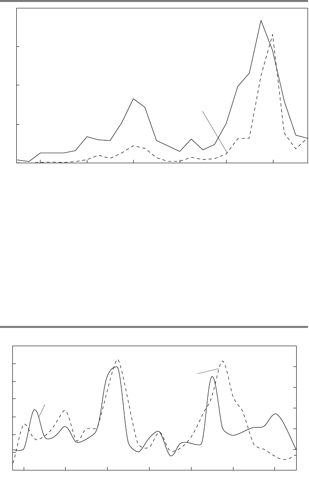
historical average by 2004, and the narrow spreads persisted through the

ﬁrst half of 2007. This could be interpreted as indicating either low expec-

tations of default or unusually high risk tolerance. A factor that points to the

latter is the sharp increase in speculative-grade debt outstanding over the

same period, suggesting that rating agencies expected higher default rates.

As my ﬁgure 3 shows, speculative-grade corporate debt issuance is a lead-

152 Brookings Papers on Economic Activity, Fall 2008

Figure 2. Defaults on Corporate Bonds, 1980–2005

Source: Moody’s.

1982 1986 1990 1994 1998 2002

150

100

No. of issues defaulting

Default volume

(billions of dollars)

Figure 3. Originations of and Default Rates on Speculative-Grade Debt, 1981–2008

Sources: Standard & Poor’s Global Fixed Income Research; Standard & Poor’s CreditPro.

1982

Percent Percent

Default rate on

speculative-grade

debt (right scale)

New B- and lower

debt as share of all

speculative-grade debt

(left scale)

1986 1990 1994 1998 2002 2006

11472-02b_Gerardi-Comment_rev.qxd 3/6/09 12:25 PM Page 152

COMMENTS and DISCUSSION 153

ing indicator of default rates on speculative debt generally. By analogy,

investors should have been able to infer that the sharp increase in sub-

prime originations would have a similar effect on defaults in the mortgage

market. In fact, the emergence of a fully private subprime lending market

can itself be interpreted as arising from increased risk tolerance, since

before 2000 most subprime loans carried Federal Housing Administration

guarantees.

This body of evidence, together with the ﬁndings in this paper, leads me

to conclude that unusually high risk tolerance was likely to have been more

important than a misperception of risk to the rapid growth in subprime

lending and to the crisis that followed.

COMMENT BY

NICHOLAS S. SOULELES Kristopher Gerardi, Andreas Lehnert,

Shane Sherlund, and Paul Willen have assembled a number of rich mort-

gage datasets and carefully analyzed them to address some important issues

at the center of the current ﬁnancial crisis. In particular, could (and should)

analysts have predicted the recent surge in home foreclosures? The paper’s

answer to this question has three main parts. First, the declines in home

prices and housing equity were the key drivers of the foreclosures; other

factors such as underwriting standards did not deteriorate enough to explain

them. Second, the strong sensitivity of foreclosures to home prices was pre-

dictable in advance. Third, analysts must therefore have believed that there

was little chance of a large decline in home prices. I will start by discussing

the ﬁrst two arguments and the paper’s empirical analysis of mortgage

defaults. To summarize, although it is not necessary to run a “horserace”

between home prices and underwriting standards, the empirical analysis

provides compelling evidence that one could have predicted that a large

decline in home prices would lead to a signiﬁcant increase in defaults. This

is an important result. But what the result implies for home price expecta-

tions is a more subtle issue.

THE ANALYSIS OF MORTGAGE DEFAULTS. First, underwriting standards

could potentially have played a larger role than implied by the paper’s

results. Figure 3 of their paper shows that underwriting standards declined

along numerous margins, and there could be important interactions across

those and other margins. To illustrate, the top left panel of ﬁgure 4 shows

that through 2005 the probability of default for low-documentation (low-

doc) loans was similar to that for full-documentation loans, but after 2005

the probability of default rose much more for the low-doc loans. This

11472-02b_Gerardi-Comment_rev.qxd 3/6/09 12:25 PM Page 153

154 Brookings Papers on Economic Activity, Fall 2008

suggests that some other factor that interacts with low-doc loans deterio-

rated after 2005. The key question is whether this factor is (mainly) the

decrease in home prices. There are other, not mutually exclusive, possibil-

ities. Suppose that before the housing boom, lenders were more likely to

offset the risk associated with low documentation by reducing risk along

other margins; for instance, by relying more on lower loan-to-value (LTV)

ratios, or on higher credit scores, traditional amortization, or other positive

risk factors. This would have reduced the overall risk of low-doc loans in

the past. Conversely, there might have been more observations of bad

combinations of risk factors (for example, low documentation and low

scores) in recent years. The point is that underwriting standards have many

components, and they can endogenously interact. In that case one cannot

simply introduce the individual components separately into an empirical

model. The paper recognizes this point and includes some interaction

terms (“risk layering”), but only a few; these are mostly interactions with

LTV and are mostly limited to the ﬁrst default model, the probit model

reported in their table 5. In this sense the results provide a lower bound on

the importance of underwriting standards. It would be interesting to know

what greater proportion of defaults could be explained by including more

interaction terms—indeed, as saturated a set as possible.

Further, although the paper’s datasets are rich in information about bor-

rowers and their mortgages, this is still only a subset of the information

available to lenders for assessing their loans. For instance, the datasets lack

information on some contract terms, such as points and fees; some applica-

tion data, such as the borrowers’ ﬁnancial wealth; and some credit bureau

data, such as past mortgage payment problems. Such information, which is

known by lenders, could potentially have been used to predict even more

of the increase in defaults.

Second, it is not necessary to think of the paper’s exercise as a horserace

between underwriting standards and home prices. To begin with, in non-

linear models generally there is no unique decomposition of the impor-

tance of individual explanatory variables. More substantively, if home

prices interact with underwriting standards and other factors, it is inher-

ently difﬁcult to quantify the relative importance of home prices per se.

For example, a number of studies have found that low equity interacts with

1. For example, David Gross and Nicholas Souleles, “An Empirical Analysis of Per-

sonal Bankruptcy and Delinquency,” Review of Financial Studies 15, no. 1 (2002): 319–47,

using an administrative dataset containing all the key variables tracked by credit card

lenders, analyze the increase in consumer bankruptcy and credit card default in the late

1990s.

11472-02b_Gerardi-Comment_rev.qxd 3/6/09 12:25 PM Page 154

COMMENTS and DISCUSSION 155

2. See, for example, Christopher Foote, Kristopher Gerardi, and Paul Willen, “Nega-

tive Equity and Foreclosure: Theory and Evidence,” Journal of Urban Economics 64,

no. 2(2008): 234–45. To illustrate, consider the polar case in which default occurs if and

only if the borrower both has negative equity and becomes unemployed. Foote and his coau-

thors ﬁnd that borrowers with negative equity in recent years are more likely to default than

borrowers with negative equity were in 1991 (before the growth in subprime loans), ceteris

paribus. Using the ABS data in this paper, but without ending the sample in 2004, Shane M.

Sherlund, “The Past, Present, and Future of Subprime Mortgages,” Staff Paper 2008-63

(Washington: Federal Reserve Board of Governors, 2008), ﬁnds that borrowers with ﬁxed-

rate mortgages were less signiﬁcantly sensitive to negative equity than were borrowers with

adjustable-rate mortgages, ceteris paribus. Such results suggest that net equity might interact

with other factors, such as the characteristics of borrowers or their mortgage terms.

3. See, for example, Gary Gorton, “The Panic of 2007,” working paper (Yale Univer-

sity, 2008).

“triggers” such as unemployment spells.

Such triggers can also be corre-

lated with underwriting standards; for example, unemployment risk could

be correlated with a low credit score.

A larger role for declines in underwriting standards (or for other factors)

can still be consistent with the overall argument of the paper, so long as

these declines were largely observable or predictable, and so long as home

prices were a predictably signiﬁcant factor in generating default. If recent

subprime mortgages were even more risky, and predictably so, the argu-

ment would be that this implied even more optimism about future home

prices. Pushing the argument further, many of the subprime mortgages

might have been unviable unless the borrowers could eventually reﬁnance

out of them, which presumes positive-enough net equity and high-enough

home prices.

The paper does provide compelling evidence about the predictable sig-

niﬁcance of housing equity for mortgage default. (One small quibble: The

paper contends that analysts could have used the results for low-but-

positive equity in 2000–04 to quantitatively extrapolate the effects of

negative equity after 2004. This extrapolation depends, of course, on the

assumed functional form, and analysts could not have known ex ante

which functional form would have worked well.) As for the effects of

underwriting standards, to the extent that there were few observations in

the early data of some of the bad combinations of risk factors that became

salient later (perhaps, for example, low documentation combined with low

credit scores), it would have been more difﬁcult to forecast future default

rates with precision. In fact, the main default model applied to the ABS

data (the competing-risks model reported in table 10) could not include

some salient mortgage characteristics—not even the uninteracted effects

of nontraditional amortization, or of negative equity (that is, a nonlinear

11472-02b_Gerardi-Comment_rev.qxd 3/6/09 12:25 PM Page 155

effect for low equity, in addition to the included linear equity variables)—

since there were too few observations of mortgages with those characteris-

tics in the ABS data before 2004.

IMPLICATIONS FOR HOME PRICE EXPECTATIONS. Supposing it was pre-

dictable that large declines in home prices would lead to large increases in

default rates, can one therefore conclude that lenders and other analysts

must not have been expecting large declines in home prices? There are

again alternative, not mutually exclusive, possibilities.

First, without complete information on the terms of the mortgage con-

tracts, it remains possible that lenders thought they were offsetting some-

what more of the mortgage risk than implied by the analysis. Second,

lenders and investors might have been willing to tolerate some nonnegligi-

ble risk of a large decline in home prices, if their risk aversion was low

enough and they considered alternative outcomes (such as a period of stag-

nant home prices) sufﬁciently likely. Third, insofar as agency problems

were important, some lenders might have thought that they would not fully

bear the costs of the increased defaults, even if they could have predicted

them.

To investigate this possibility, one would ideally like to distinguish

the information set of the mortgage originators from the information sets

of investors and other agents, which presumably are subsets of the former,

to see whether the additional information available to the originators

would have predicted signiﬁcantly more of the defaults.

Finally, even if analysts should have been able to predict much of the

increase in mortgage defaults, it would have been more difﬁcult to forecast

their spillover onto the rest of the ﬁnancial system and the extent of the

resulting crisis, and moreover to forecast how the crisis in turn would spill

back into the mortgage market, further increasing defaults through even

lower home prices and other mechanisms (such as higher unemployment).

Although the paper’s competing-risks models explain much of the

increase in defaults, in the end they still generally underpredict them, espe-

cially for the 2005 vintage of mortgages. The paper suggests that this could

reﬂect the fact that the 2005 vintage was more exposed than the 2004 vin-

tage to home price declines. However, the competing-risks models are

156 Brookings Papers on Economic Activity, Fall 2008

4. On this topic, see, for example, Adam Ashcraft and Til Schuermann, “Understanding

the Securitization of Subprime Mortgage Credit,” Staff Report 318 (Federal Reserve Bank

of New York, 2008); Charles Calomiris, “The Subprime Turmoil: What’s Old, What’s New,

and What’s Next,” working paper (Columbia University, 2008); Benjamin Keys and others,

“Securitization and Screening: Evidence from Subprime Mortgage Backed Securities,”

working paper (University of Michigan, 2008); and Atif Mian and Amir Suﬁ, “The Conse-

quences of Mortgage Credit Expansion: Evidence from the 2007 Mortgage Default Crisis,”

working paper (University of Chicago, 2008).

11472-02b_Gerardi-Comment_rev.qxd 3/6/09 12:25 PM Page 156

COMMENTS and DISCUSSION 157

supposed to control for the effects of lower home prices through lower

housing equity (and for the resulting decline in the borrower’s ability to

reﬁnance the mortgage or sell the home instead of defaulting). How

much larger a share of the observed defaults could be explained through

improved measurement and modeling of housing equity remains an open

question. Perhaps other relevant risk factors are still missing from the

model, or perhaps the increase in defaults was to some degree inherently

difficult to predict in advance, even given the path of home prices.

Nonetheless, the paper has made a valuable contribution in showing that

home prices were in any case a predictably signiﬁcant contributor to the

defaults.

GENERAL DISCUSSION Jan Hatzius remarked that the idea that peo-

ple incorrectly guessed the direction of home prices but not the relation-

ship between home prices and defaults was consistent with his impression

from discussions he had had with market analysts over the past few years.

Most refused to believe, despite a history of large regional declines in

home prices, and of nationwide declines in other countries, that home

prices in the United States could decline in nominal terms. This denial, he

believed, was the essential problem that led to the crisis.

Karl Case stressed the importance of examining the data at the regional

level. What was happening in Florida, Nevada, and Arizona, for example,

was very different from what was occurring in the Midwest and the North-

east. California’s situation was particularly notable since that state accounts

for 25 percent of the nation’s housing value and experienced a steep decline

in prices. He added that the laws relevant to housing differ in important

ways from state to state, and that markets clear at different rates in differ-

ent areas.

Austan Goolsbee offered an airline analogy to illustrate how the crisis

arose largely from the interaction of declining home prices and deterio-

rating lending standards, with the latter playing the lead role. To enable

people with bad credit to buy homes, the financial markets had created

subprime mortgages and other products that translated home price appreci-

ation into broader home ownership. Just as ﬂying on a budget airline is ﬁne

until something goes wrong, so these subprime mortgages were ﬁne until

prices started to fall. Goolsbee added that the securitization of those mort-

gages was much more complicated than what the paper portrayed, and that

lending standards deteriorated not only through the relaxation of lending

criteria but also through outright fraud: people were allowed to lie about

11472-02b_Gerardi-Comment_rev.qxd 3/6/09 12:25 PM Page 157

the owner-occupier status of the home they purchased. This matters

because people are more likely to walk away from a second home than

from a primary residence as soon as they fall into negative equity. Lenders

should have assumed that the market would go bad at some point and

priced their loans accordingly.

Frederic Mishkin noted that the adjustable subprime contracts inher-

ently assumed a rise in asset prices, because otherwise the loans would not

continue to be serviced when the interest rate was reset. Lenders assumed

that prices would continue to rise, turning subprime borrowers into prime

borrowers, who could then reﬁnance the loan on better terms. He indicated

that loans made with the expectation that they would be reﬁnanced may

have been prompted by underlying principal-agent issues.

Robert Hall mentioned the work of John Campbell and Robert Shiller

showing that overvaluation in a stock market can be detected by looking at

the price-dividend ratio: the higher the ratio, the higher the likelihood of a

price decline. He suggested incorporating this type of analysis into the

paper by looking at price-rent or price-income ratios, noting that their

unprecedentedly high levels in the mid-2000s signaled a high probability

of future decline.

Martin Baily directed the Panel’s attention to the prices of ABX

securities—the collateralized debt obligations built on the mortgage-

backed securities—and to delinquency rates, which, he argued, revealed a

likely change in underwriting standards in the years before the crisis. ABX

securities declined signiﬁcantly in price between the ﬁrst and the second

quarters of 2006, too short an interval to be explained by a drastic change

in the underlying mortgages. Delinquency rates, in contrast, increased

sharply in the fourth quarter of 2005 and continued to rise in subsequent

quarters. The dissimilarity between these two data series seems to indicate

a change in something other than housing prices, such as underwriting

standards.

Charles Schultze summarized the paper as saying that analysts did

understand the nonlinear dependence of foreclosures on changes in home

prices but were shocked by the idea that home prices would fall as much as

they did. He attributed the unusual size of the price drop to the fact that

there had not been an upward movement in home prices this large in the

previous forty years. He blamed the incentive structure facing the man-

agers and employees of ﬁnancial ﬁrms: one’s approach to risk manage-

ment changes if one can expect bonuses for four or ﬁve years on the upside

and only miss one or two on the inevitable downside. He cited a UBS

report written after the bank lost the ﬁrst $19 billion of $42 billion in even-

158 Brookings Papers on Economic Activity, Fall 2008

11472-02b_Gerardi-Comment_rev.qxd 3/6/09 12:25 PM Page 158

COMMENTS and DISCUSSION 159

tual losses, in which the downplaying of risk management is noted. In

addition, the lack of attention to risk evaluation by investors generated a

surge in demand for subprime mortgage-backed securities that put pressure

on mortgage originators for a substantial erosion of underwriting standards.

Lawrence Summers noted the long tradition of ﬁnancial messes made

because people observed that over a long period the strategy of writing

out-of-the-money puts had proved consistently proﬁtable, and so contin-

ued the strategy until inevitably a problem occurred. He seconded Gools-

bee’s comment on the interaction of factors deepening the crisis and asked

the authors to try to tease out these different factors. He also suggested that

the authors examine the strategies pursued by major builders, the stock

prices of those builders, and the implied volatility in puts on their stocks,

since builders are essentially betting their franchises on the housing busi-

ness remaining strong. He guessed that such an examination of these fac-

tors would show that the builders shared in the euphoria of rising home

prices yet did not share in the ignorance—an idea at odds with Schultze’s

emphasis on Wall Street’s compensation structures.

Bradford DeLong came to the defense of those who had bought homes in

California, Florida, and Boston, arguing that long-term interest rates will

eventually decline, leading to an increase in home price–rent ratios. Also,

rising population in the United States will eventually lead to increased con-

gestion, so land will essentially become a Hotelling good with prices rising

over time.

Richard Cooper remarked that one should not limit one’s analysis of

home price–income ratios to a period of worldwide decline in real long-

term interest rates, because housing is a long-term asset. He also pointed out

that, at least in the United States, the income elasticity of demand for hous-

ing is signiﬁcantly greater than one, so that rising incomes would eventually

lead to an increase in home price–income ratios. But it would be too sim-

plistic to make an evaluation from this ratio alone.

11472-02b_Gerardi-Comment_rev.qxd 3/6/09 12:25 PM Page 159

11472-02b_Gerardi-Comment_rev.qxd 3/6/09 12:25 PM Page 160