
Office of Portfolio Analysis
OPA_T#973_Mar-23-2016
OPA Excel Tips: Merging in data from another sheet (VLOOKUPs)
There are a number of situations where it is helpful to merge two datasets or copy a variable
from one dataset to another. The VLOOKUP function in Excel is a very handy way to do this.
A VLOOKUP looks for a specified value in an array of data (usually in another worksheet or
workbook), and returns the value from a specified column. (HLOOKUP is the same but looks for
rows)
The VLOOKUP command requires four pieces of information:
Look up value: The value you want to look up e.g. and Application ID. This is usual a cell
reference and changes for each line of the dataset. It is possible to look up any cell value
(text or numeric) but the method is most reliable when using an ID number as text (e.g.
institution name) may have different spellings or a space after the final letter for example.
These differences would prevent Excel from making the match.
It is also important to consider the two datasets you are using e.g. if there are multiple
rows per project number Excel will just copy across the value from the first match.
Table array: the dataset that you want to look to for the variable of interest. This needs to
include the value you are looking up in the leftmost column e.g. if you were looking up
based on ApplID, the first column of the array would need to contain ApplID. This doesn’t
need to be the first column on the worksheet though.
Column number: The number of the column in the array that contains the variable you are
interested in. This is independent of the number of columns in the spreadsheet e.g. if the
array you select is columns B to D and the variable is in column D, you would instruct the
VLOOKUP to use column 3.
Range lookup: Enter ‘false’ to ensure Excel searches for an exact match for the lookup
value.

Office of Portfolio Analysis
OPA_T#973_Mar-23-2016
Example 1: Merging Application Status onto the Transplantation dataset.
In this example the Transplantation dataset is used.
Assume we want to add on the project status and institution e.g. to find out how many of the
applications have been awarded and that we have this data in a separate Excel file. In this
example it would be possible to download a complete new dataset from QVR but it isn’t always
this straightforward, for example you may have a manually curated flag to indicate how long an
institution or PI has been receiving funding from your IC and want to attach that to a QVR
dataset.
An Excel file with Institution name and application status is shown below. It is also available on
the OPA training pages as Transplant_Inst_Status_data.

Office of Portfolio Analysis
OPA_T#973_Mar-23-2016
Note both datasets have similar identifying variables (Application ID, Project number) which are
vital to enable VLOOKUPs to work.
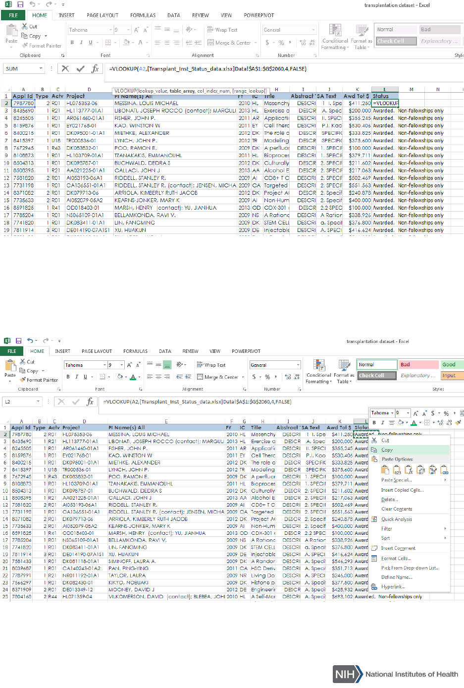
Step 1. Add header to new column
Next enter the VLOOKUP formula in cell. The formula is:
=vlookup([cell with ID value of interest],[group of cells to look to for values],[Column number of
interest],False)
So in this instance, we want to look up based on ApplID so in cell L2, the value to look up is held
in cell A2.
The group of cells (array) we’re interested in is in the Transplant_Inst_Status_data worksheet,
and needs to have ApplID as the first column (though it doesn’t have to be the first column in
the worksheet). Selecting columns A to G as the array ensures ApplID is in the first column and
we can then select any of the values in the dataset to pull across to the Transplantation dataset.
Status is in column D, the fourth column in the array selected, so we put column ‘4’ into the
formula.
Before copying the formula to the entire column, make sure that there are ‘$’ symbols before
the letters and numbers in the array cell references, otherwise when copying and pasting the
array may change. The ‘$’ symbol tells Excel to fix the column and row values in the formula.
When using an array in a different workbook, Excel does this automatically, when referring to a
different worksheet in the same workbook, you need to do it manually.
Office of Portfolio Analysis
OPA_T#973_Mar-23-2016
Example 2: Merging Institution onto the Transplantation dataset.
If you have worked through the first example, you can copy and paste the formula from cell L2
into cell M2.
This gives an error message as it’s looking for the value in cell B2 in the ApplID column in the
Transplant_Inst_Status_data sheet, which doesn’t exist.

Office of Portfolio Analysis
OPA_T#973_Mar-23-2016
Change the value ‘B2’ to ‘A2’. You can get round this by putting a ‘$’ in front of the A to ensure
that Excel keeps the column A in the formula when you copy and paste. Also change the column
to copy over from ‘4’ which contains the status description to ‘6’ which contains institution
name.
In this example you could also use project number to match the same information across using
these datasets. The formula to match on Institution would be:
=vlookup(D2,[Transplant_Inst_Status_data.xlsx]Data!$B$1:$F$2060,5,false)

Office of Portfolio Analysis
OPA_T#973_Mar-23-2016
Note we’re now using column D to identify the value to look up and the array has changed to
columns B to F.
More help
Click in the formula box, on ‘vlookup’, this will bring up the pop up box shown below with a
hyperlink to the Excel VLOOKUP help text.
