
1
Penning- och valutaPolitik 2018:2
Sweden’s scal framework and monetary policy
Eric M. Leeper*
The author is Professor of Economics at the University of Virginia
Basic economic reasoning tells us that monetary and scal policies always
interact to jointly determine aggregate demand and the overall level of
prices in the economy. This arcle interprets Sweden’s explicit monetary and
scal frameworks in light of this reasoning, bringing recent Swedish inaon
and interest-rate developments to bear on the interpretaons. Theory and
evidence raise the queson of whether the two policy frameworks are mutually
consistent.
1 Introducon
Basic economic reasoning tells us that monetary and scal policies necessarily interact
in the short, medium, and long runs. These interacons jointly determine an economy’s
macroeconomic developments. This reasoning is completely general, independent of any
parcular economic model or view of how the economy operates.
Most countries’ monetary and scal policy instuons, in contrast, are founded on the
presumpon that the two policies can and should operate independently of each other. This
presumpon underlies the creaon of central banks that are given well-specied mandates
to control inaon and stabilize the real economy and to operate in isolaon from pressures
that might emanate from scal authories. Fiscal policy, meanwhile, is assigned the task of
stabilizing debt – what is called ‘sustainable scal policy’ – and oen lile else. Underlying
this instuonal construct are the beliefs that
(i) scal policy has lile, if any, impact on inaon;
(ii) monetary policy has negligible scal consequences;
(iii) the single-minded scal pursuit of debt stabilizaon supports, rather than thwarts,
the central bank’s mandates.
Somemes, this instuonal arrangement works. At other mes, the arrangement leads to
monetary and scal policies that are mutually inconsistent.
The presumpon that policies can and should operate independently denies an essenal
fact about modern public nance: governments issue nominal bonds – bonds denominated
in local currency – but bondholders care about the real value of those bonds. The real value
comes from deang nominal debt by the overall level of prices in the economy, something
like the consumer price index. Because modern central banks aim to target the rate of
change of the price level – the inaon rate – it is impossible to separate monetary and scal
policy completely. And eorts to do so can create policy conicts.
Recent Swedish monetary and scal acons illustrate the possibility of conict. At
a me when monetary policy has been aggressively expansionary in an eort to raise
inaon – negave policy interest rates for three years, coupled with signicant asset
purchases that have produced a more than four-fold increase in the central bank’s balance
sheet from 2007 to 2017
1
– scal policy has become more contraconary, with net lending
1 Total assets more than tripled between the third quarter of 2008 and the rst quarter of 2009 and remained elevated unl
the second half of 2010. Assets have nearly doubled over the negave policy rate period beginning in 2015.
* I thank Campbell Leith and Todd B. Walker for discussions and the Swedish Fiscal Council, Rachel Lee, and Jesper Lindé for
detailed comments. I also thank Hannes Jägerstedt for paently gathering data and explaining them to me. The opinions expressed
in this arcle are the sole responsibility of the author. They should not be interpreted as reecng the views of Sveriges Riksbank.

Sweden’S fiScal framework and monetary policy
2
moving from −1.6 percent of GDP in 2014 to 1.2 percent in the rst two quarters of 2017.
Fiscal policy has been deaonary when monetary policy has been inaonary.
Sweden is a fascinang case to study how monetary and scal policies interact to
inuence the aggregate economy. The country stands out for being explicit about the
objecves and targets of its macroeconomic policies. Sveriges Riksbank, Sweden’s central
bank, exibly targets inaon at two percent, while the government currently pursues a
medium-term net-lending target of 1 percent of GDP. Explicitness makes Swedish policy
behavior amenable to assessment, which is one goal of this arcle. I raise the possibility that
the policy rule that Swedish scal authories follow, parcularly in recent years, may be at
odds with the Riksbank’s primary goal of targeng inaon.
1.1 Targets vs. rules
Explicit policy targets are not sucient to ensure eecve policy performance. Central
banks with explicit inaon targets communicate much more than their target to the public.
There are innitely many ways that the Riksbank could try to achieve its two percent target.
Each way – or ‘policy rule’ – aects private-sector expectaons dierently. Each rule and its
associated expectaons has unique impacts on the public’s economic decisions. To reduce
the likelihood of mistaken public expectaons, the Riksbank communicates the parcular
rule that it tries to follow.
Communicang the rule is challenging. To achieve its inaon target, the Riksbank
analyses a vast array of data – domesc and foreign inaon and real economic
developments and forecasts, current and prospecve values of the krona, public and
nancial market expectaons of inaon, and even polical events at home and abroad.
2
By
describing how these facts and conjectures inuence its choice of the path for the repo rate,
the Riksbank is explaining its policy rule: how the central bank reacts to various kinds of news
that aect Swedish inaon and real acvity. Of course, the Riksbank, and no central bank,
follows a simple algebraic rule that can be precisely and succinctly communicated. But it
does respond systemacally to economic condions and that systemac behavior guides the
public’s formaon of expectaons about future monetary policy acons.
The Swedish government’s net-lending target, while commendable from the viewpoint
of scal sustainability, does nothing to communicate the scal behavior that tries to achieve
the target. Dierent governments are free to choose exactly how and when to hit the target;
the same government can choose dierent methods for achieving the target at dierent
points in me. This is a potenally serious shortcoming of Sweden’s scal framework, a
shortcoming shared by governments the world over. Governments can perhaps be forgiven
for confounding rules and targets. Even the Internaonal Monetary Fund uses the term ‘rule’
to describe scal targets and restraints, rather than to characterize how the scal authority
behaves.
3
Because this arcle focuses on how interacons among scal, monetary, and public
behavior determine the economy-wide price level, to avoid confusion I will delineate
between targets and rules. Targets refer to inaon at two percent and net lending at
one percent, while rules describe the policy behavior that achieves those targets. A rule
characterizes how the choice of a policy instrument – the repo rate, tax rates, expenditure
components – depends on prevailing economic condions. I argue that the policy rules are
all-important for determining the price level and, by extension, the performance of the
macro economy.
2 See Sveriges Riksbank (2018, chapter 1) for examples.
3 Schaechter et al. (2012).

3
Penning- och valutaPolitik 2018:2
1.2 Sketch of arcle
Before geng into details about Sweden, it is necessary to lay some groundwork for
understanding how and why it is essenal to study monetary and scal policies together,
rather than separately. To that end, I describe the nature of policy interacons in any well-
funconing equilibrium. Fundamental economic principles carry some crical implicaons
that conict with beliefs (i)–(iii). First, it is the joint monetary-scal policy regime that
determines an economy’s inaon rate. Second, monetary policy acons always have scal
consequences – consequences that may be large at mes – and how scal policy reacts to
those consequences maers for the ulmate impacts of the monetary policy acons. Finally,
the rule that the government implements to pursue debt stabilizaon maers for the central
bank’s ability to achieve its mandates.
With that economic background in place, the arcle turns to analyse features of Swedish
macroeconomic policies and recent Swedish economic developments. These include
1. negave bond yields over the maturity structure, which constute prima facie
evidence of a scal policy that reduces social welfare, but also reect the low-interest
rate environment in which the Swedish economy nds itself;
2. the fragility – in the sense of potenally inducing instability in government debt – of
Sweden’s net-lending target, for reasons rst arculated by Phillips (1954);
3. evidence of Swedish scal policy behavior and the backing that it provides for
monetary policy;
4. an explanaon of how, parcularly in low-inaon periods, monetary policy acons
can generate potenally substanal scal impacts in subtle ways that are not part of
typical economic analyses at central banks and ministries of nance.
The arcle’s aim is not to cricize Swedish policies. Sweden’s scal situaon is sound:
the government owns equies and its net nancial posion is posive. But the Swedish
government nonetheless issues krona-denominated debt, so the analysis in this arcle
applies to Sweden, as it would to less scally sound economies. The arcle tries to shed light
on how monetary and scal policies in Sweden jointly determine macroeconomic outcomes.
Along the way, the arcle points toward alternave scal rules that are consistent with the
aims of Sweden’s Fiscal Policy Framework and are more compable with the job that the
Riksbank has been tasked to perform.
2 Monetary and scal policy basics
Much discourse about macroeconomic policies applies the following logic. The central bank
sets its policy instruments – a short-term nominal interest rate, the level of bank reserves,
the size and composion of its balance sheet – but does not set taxes and government
expenditures. The government chooses the level and composion of various taxes and
expenditures and the quanty and maturity structure of the debt it issues, but not the
variables the central bank controls. Having established who controls what, analyses of policy
impacts oen proceed along similar lines to ask: How do changes in the central bank’s
(government’s) instruments aect the economy, holding xed scal (monetary) instruments?
Although such quesons seem to make sense on the surface, basic economic reasoning
tells us that it is rarely possible to change a monetary (scal) instrument without eventually
changing scal (monetary) instruments in parcular ways.
Research over the past 25 years establishes this reasoning to emphasize that monetary
and scal policy jointly determine the economy-wide level of prices and the rate of inaon.
4
4 Early contributors include Leeper (1991), Sims (1994), Woodford (1995), and Cochrane (1999). Leeper and Walker (2013)
and Leeper and Leith (2017) are recent overviews. Leeper (2016) explains why central banks – even when they are polically and
operaonally independent – need to pay aenon to scal behavior.

Sweden’S fiScal framework and monetary policy
4
Out of that literature has emerged the understanding that two disnct combinaons of
monetary and scal policy behavior – policy regimes – can determine the price level and
stabilize the level of government debt.
2.1 Policy regimes
Table 1 summarizes the policy mixes that determine inaon and stabilize debt. To make
the arguments clear, I make stark and unrealisc assumpons about policy behavior. The
arguments go through with more plausible assumpons.
The rst regime reects the convenonal view that monetary policy acvely adjusts
the policy interest rate to lean against inaon, while scal policy passively adjusts
primary budget surpluses – revenues less expenditures, not including interest payments
on government debt – to stabilize the long-run debt-GDP rao. This is somemes called
‘monetary dominance.’ Taylor’s famous rule
5
falls into this regime: the central bank raises
the policy interest rate more than one-for-one with the inaon rate and raises the interest
rate more modestly when the output gap increases.
6
Because monetary policy focuses on
stabilizing inaon and the real economy, scal policy must ensure that government debt
remains well behaved. When scal policy makes taxes rise with the level of real government
debt – nominal debt deated by the price level – by more than enough to cover interest
payments and some of the principal, the debt-GDP rao will be stable in the long run.
Many economists believe this regime prevails during ‘normal’ economic mes. All inaon-
targeng central banks believe they operate in this regime.
Table 1. Monetary-scal policy mixes
Policy authority Monetary-scal policy regimes that determine inaon and stabilize debt
Monetary rule
Fiscal rule
Conventional view
Aggressively raises interest rate with inaon
Raises primary surplus with real debt
Alternave view
Weakly raises interest rate with inaon
Pursues other objecves besides debt
stabilizaon
Label ‘Acve monetary passive scal policies’
or ‘Monetary dominance’
‘Passive monetary acve scal policies’
or ‘Fiscal dominance’
A second, alternave, regime can also determine inaon and stabilize debt. In this regime,
scal policy pursues other objecves, such as countercyclical policies or redistribuon of
income, by seng primary surpluses – dened as tax revenues less expenditures, excluding
interest payments on outstanding debt – independently of debt and the price level.
Monetary policy chooses the interest rate so that it responds only weakly – or not at all – to
inaon, which permits expansions in government debt to raise the price level. Higher price
levels and lower bond prices reduce the real market value of debt – the quanty of goods
and services that a government bond can purchase – to make the debt-GDP rao stable.
Some economists call this regime ‘scal dominance.’
At a general level, there is nothing ‘good’ or ‘bad’ about the two policy regimes. Recent
research on jointly opmal monetary and scal policies nds that the best mix of policies in
terms of social welfare has elements of both the convenonal and the alternave views.
7
Both regimes deliver the broad macroeconomic policy goals of determining inaon and
stabilizing government debt. But because monetary and scal acons have dierent impacts
in the two regimes, it is essenal for policymakers to know in which regime the economy
resides.
5 Taylor (1993).
6 For reasons rst arculated by Obseld and Rogo (1983), monetary policy cannot deliver a unique inaon rate in a pure at
currency regime. Cochrane (2011) and Sims (2013) recently emphasized that the Taylor rule permits explosive inaon paths to
be equilibria, along with the stable inaon outcome that economists usually focus on.
7 Sims (2013) and Leeper and Zhou (2013).

5
Penning- och valutaPolitik 2018:2
Because U.S. monetary policy behavior was been widely studied, I will point out several
instances since America le the gold standard in April 1933 in which the Federal Reserve
seems to have followed this alternave behavior: from April 1933 unl about 1936;
throughout World War II unl the Treasury-Fed Accord in March 1951; much of the 1970s;
the 2008 nancial crisis and its aermath.
8
And there have been mes when scal policy
pays scant aenon to debt in order to pursue other objecves: despite extremely high
war debt, in 1948 Congress overrode President Truman’s veto and cut taxes; the Economic
Recovery Plan of 1981 increased primary decits even as the debt-GDP rao was rising from
its post-war low in the early 1980s; both the Economic Growth and Tax Relief Reconciliaon
Act of 2001 and the Jobs and Growth Tax Relief Reconciliaon Act of 2003 cut taxes at mes
of rising debt; the American Recovery and Reinvestment Act of 2009 increased spending and
cut some taxes despite rising debt; even with record peaceme government debt levels, in
December 2017 the U.S. government passed a major cut in taxes.
9
During and since the nancial crisis of 2007, central banks around the world have
maintained policy interest rates that are pegged at extraordinarily low levels with the aim of
smulang real economic acvity. This behavior places monetary policy into the ‘alternave
view’ category. At the same me, scal policies – parcularly in Europe – have been adjusng
to stabilize government debt following brief excursions into smulave stances designed to
help li economies out of recession. By Table 1’s categorizaons, the mix of pegged interest
rates and stabilizing scal policy, if people expect it would last forever, does not deliver an
equilibrium in which inaon is determined.
10
2.2 Fiscal consequences of monetary policy
To keep this discussion focused, in what follows I consider only the convenonal mix of
monetary and scal policy behavior. That policy combinaon underlies the Riksbank’s
percepons of its behavior and the raonale for Sweden’s Fiscal Policy Framework. The
independent Riksbank pursues its inaon target, while the government acts to ensure debt
is stable. This convenonal view of macroeconomic policies is the foundaon of monetary
and scal instuons in nearly all countries.
My key message is: under this convenonal policy mix, monetary and scal policies
must interact in certain well-specied ways. It is not possible for monetary and scal policy
to operate independently of each other and sll deliver good economic performance.
Understanding the nature of these interacons is essenal to formulang eecve policy
rules.
Monetary policy acons always have scal consequences.
11
Let’s start with something
roune: the Riksbank lowers the repo rate in order to raise inaon. This isn’t the end of the
story: a lower repo rate tends to lower all interest rates, including those on government debt,
so interest payments on outstanding debt decline.
Now scal policy comes into play. Those lower interest payments reduce scal needs.
To ensure that government debt is stable, taxes must be lower or expenditures must be
higher in the future to oset the reduced debt service. Without these scal adjustments,
government debt would steadily fall, eventually making the government a net lender to the
private sector.
But there is actually more to the scal response than simply stabilizing debt. Lower
interest payments on government bonds reduce the wealth of holders of those bonds. If
8 See Taylor (1999), Clarida et al. (2000), Lubik and Schoreide (2004), and Davig and Leeper (2006, 2011).
9 See Davig and Leeper (2006), Bhaarai et al. (2016), and Bianchi and Ilut (2017).
10 This is called ’price-level indeterminacy,’ and is a topic that has received a great deal of aenon in the academic literature.
Indeterminacy means that the inaon rate is not pinned down by policy and is subject to potenally volale uctuaons that
arise from self-fullling expectaons of inaon by the private sector. Woodford (2003) explains that determinacy is a minimal
requirement for opmal policy.
11 Tobin (1980) and Wallace (1981) make this point.

Sweden’S fiScal framework and monetary policy
6
those lower interest receipts do not trigger an expectaon of eventually lower taxes to
compensate for the reduced wealth, lower wealth will lead to reduced demand for goods
and services – lower aggregate demand – and a lower price level.
Because the Riksbank inially reduced the repo rate in the hope of raising aggregate
demand and inaon, the negave wealth eect can thwart the Riksbank’s eorts. To
support monetary policy, scal policy needs to provide scal backing that adjusts future
taxes in the opposite direcon to price-level movements. A higher price level – the Riksbank’s
immediate goal – requires a scal rule that lowers future taxes, while a lower price level
calls for a policy that raises taxes. Such a rule eliminates the wealth eects of central bank
changes in interest rates to deliver the desired eect of monetary policy on aggregate
demand.
The scal rule under the convenonal view in Table 1 both stabilizes debt and provides
the necessary scal backing for monetary policy. A rule that raises future surpluses whenever
real debt increases has two components to it. First, for a xed price level, higher nominal
debt brings forth higher surpluses to ensure government debt is stable. Second, for a xed
level of nominal debt, a lower price level creates the expectaon of higher future taxes to
provide the scal backing for monetary policy’s inaon-targeng acons. The passive policy
rule in the table happens to deliver both desirable outcomes.
The message is: to successfully raise inaon, the Riksbank’s looser monetary policy
(lower repo rate) necessarily requires looser scal policy (smaller budget surpluses) at some
point. That scal response is essenal for the Riksbank to be able to control inaon and
fulll the price-stability policy mission that the Riksdag set out for the bank in the Sveriges
Riksbank Act.
Unfortunately, not all scal rules both stabilize debt and back monetary policy. This is
why it’s important for governments to move beyond adopng targets, toward describing
the behavior that achieves the targets. Both outcomes rely on scal expectaons. If markets
know that higher real debt eventually leads to higher stabilizing surpluses, then scal policy
will not run into sustainability problems, as investors are assured the government will fulll
its nancial commitments. This argument gures prominently in the Swedish scal policy
framework.
12
If bondholders know that lower taxes are sure to follow lower interest receipts,
then monetary policy’s adverse wealth eects will not arise, and interest-rate policy will
aect inaon as intended. This point is missing from the Swedish scal framework.
Appropriate scal backing for monetary policy is crical for the Riksbank to achieve price
stability. By giving the Riksbank the task of targeng inaon, Sweden has chosen an acve
monetary policy, which places Swedish macroeconomic policies in the monetary dominance
regime in Table 1. To be consistent with this monetary policy behavior, it is essenal that
the scal rules used to implement the target provide appropriate backing for monetary
policy. This calls for passive scal behavior. A correctly designed scal rule anchors people’s
expectaons on the belief that scal policy will, in me, react appropriately to monetary
policy by eliminang the wealth eects that monetary policy produces.
12 Swedish Government (2011), pages 5, 7, and 12, for example.

7
Penning- och valutaPolitik 2018:2
3 Internaonal examples
To gain a deeper understanding of the monetary-scal combinaons in Table 1, it is helpful to
consider actual instances when policy behavior departed from the convenonal monetary-
scal regime.
3.1 An important American case
Recovery from the Great Depression illustrates that the alternave monetary-scal policy
mix – scal dominance – has been an explicit policy choice.
13
President Franklin D. Roosevelt
took oce in March 1933 at the lowest point of the Great Depression. Compared to the third
quarter of 1929, real GNP was 36 percent lower, industrial producon had been cut in half,
unemployment rose from almost nothing to a quarter of the workforce, and the price level
had fallen 27 percent. The new president commied to raise the price level by achieving
‘…the kind of a dollar which a generaon hence will have the same purchasing power and
debt-paying power as the dollar we hope to aain in the near future’.
14
The rst step toward
permanently raising the price level was to abandon the gold standard in favor of what
Roosevelt called a ‘managed currency’.
15
Abandoning converbility of the dollar to gold included abrogang the gold clause, a
contractual provision that gave creditors the opon to receive payment in gold, on all future
and past public and private contracts. This changed the nature of government debt. Under
converbility, even though government bonds paid in dollars, the Treasury was required
to convert those dollars into gold on demand. When the Treasury didn’t have the gold on
hand, it had to acquire the gold, typically through higher taxes. The new ‘managed currency’
standard broke the automac link between new bonds and future surpluses: government
bonds were simply promises to pay dollars, which the U.S. government could freely create
without adjusng taxes.
16
Roosevelt used three strategies to convince the public that higher government debt
would not necessitate higher future taxes. First, he made policy depend on the state of
the economy, saying he would run bond-nanced decits unl the economy recovered.
Second, he emphasized the temporary nature of the policy by disnguishing between the
‘regular budget,’ which he balanced, and the ‘emergency budget,’ whose decits were
driven by spending designed to provide relief to those the depression had harmed. Finally,
Roosevelt raised the polical stakes by pitching economic recovery as a ‘war for the survival
of democracy’.
17
The strategies appeared to work because expected inaon began to rise by
spring 1933.
18
Monetary policy behaved passively through the recovery. Aer the United States le
gold, the Fed no longer needed to keep interest rates high to staunch the oulow of gold
and the New York Fed reduced its discount rate to 1.5 percent in February 1934, where it
remained unl August 1937, when it was lowered to 1 percent. One contemporary observer
wrote that the Federal Reserve ‘served merely as a technical instrument for eecng the
Treasury’s policies’.
19
Clearly, the Fed did not follow anything resembling a Taylor rule;
instead, monetary policy permied the expansion in government debt to smulate the
economy, as it does in the alternave policy mix.
Economic recovery was rapid. Real GNP returned to its pre-depression level in 1937. Price
levels – consumer and wholesale price indexes and the GNP deator – rose. The deator
regained its 1920s levels, while the other two fell somewhat short.
13 This draws on Jacobson et al. (2017).
14 Roosevelt (1933b).
15 Roosevelt (1933a).
16 Today all but the 10 percent of Treasury debt that is indexed to inaon is also merely a promise to pay future dollars.
17 Roosevelt (1936).
18 Jalil and Rua (2017).
19 Johnson (1939, p. 211).

Sweden’S fiScal framework and monetary policy
8
Historians like Friedman and Schwartz (1963) and Romer (1992) aribute recovery to
higher growth in the supply of money. Aer America le the gold standard, the Treasury
bought the gold that owed into the country from a polically unstable Europe and paid for
that gold by directly expanding bank reserves and high-powered money. But that explanaon
overlooks the signicant expansion in government debt that took place. The dollar value of
federal debt outstanding doubled in the six years aer leaving the gold standard, reecng
the substanal scal smulus associated with Roosevelt’s relief programs.
Remarkably, this expansion in nominal debt did not raise the debt-GNP rao. Figure 1
plots the par and market values of gross federal debt as percentages of GNP from 1920 to
1940.
20
The vercal line marks departure from gold in April 1933. Aer booming out in
September 1929 at 15.6 percent, the debt-GNP rao rose steadily while the United States
was sll on gold, reaching 44.7 percent in March 1933. It then remained below 45 percent
through the end of 1937. Economic recovery raised both the price level and the real level of
economic acvity, ensuring that the debt-GNP rao was stable.
10
15
20
25
30
35
40
45
50
1920 1922 1924 1926 1928 1930 1932 1934 1936 1938 1940
Figure 1. Par and market value of gross federal debt as a percentage
of GNP
Par value Market value
Note. Vercal line marks departure from the gold standard.
Sources: Hall and Sargent (2015), Balke and Gordon (1986), and authors’
calculaons
In this alternave policy mix, the Federal Reserve behaved passively, perming the scal
expansion to raise aggregate demand and with it, prices and output. With this policy mix,
there need not be any conict between scal expansion and scal sustainability because, as
the data in Figure 1 neatly illustrate, the scal expansion did not increase debt relave to the
size of the economy.
21
3.2 Recent internaonal cases
3.2.1 Brazil
Countries have not always provided appropriate scal backing.
22
In recent years, Brazil
followed a scal policy that was unresponsive to debt, while its central bank sought to
target inaon. The 1988 constuon indexed government benets to inaon, which
placed 90 percent of expenditures out of legislave control. At the same me, tax increases
were polically infeasible, leading to growing primary decits with no prospect of reversal.
When inaon began to rise, the central bank aggressively raised interest rates, just as the
20 Par value is the face value of outstanding government debt and is the most commonly cited measure of debt. Market value
incorporates current bond prices, which may change over me to aect the value of debt.
21 The Great Depression was not the only instance of this policy mix. See Davig and Leeper (2006), Erceg and Lindé (2014), and
Leeper et al. (2017) for further examples.
22 Leeper (2017) discusses these and other examples in detail.

9
Penning- och valutaPolitik 2018:2
Taylor principle instructs. Debt service rose, driving up aggregate demand and inaon. In
December 2015, the primary decit was 1.88 percent of GDP, but the gross decit – primary
plus interest payments – was 10.34 percent of output. Figure 2 plots Banco Central do Brasil’s
policy rate, the Selic, along with the consumer price inaon rate from 2013 through 2015.
Despite a doubling of the policy rate, the inaon rate rose by nearly 5 percentage points:
monetary policy does not appear to be controlling inaon. In fact, inaon began to retreat
in 2016 only aer the central bank had stabilized the Selic at 14.25 percent for a year.
3
6
9
12
15
Jan 2013 Jul 2013 Jan 2014 Jul 2014 Jan 2015 Jul 2015 Jan 2016
Figure 2. Brazilian monetary policy interest rate and consumer price
inflaon rate
Policy interest rate (Selic) Consumer price inflaon
Source: IHS Global Insight
It is tempng to infer that Brazil’s problems stemmed from dysfunconal scal policy.
Surely, if scal policy follows well-specied guidelines that ensure ‘responsible’ scal
behavior, monetary policy will be able to control inaon. In fact, the explanaon lies in an
incompable combinaon of monetary and scal policies that were both acve, in Table 1’s
nomenclature.
3.2.2 Switzerland
Switzerland has had ‘responsible’ scal targets for 15 years and it takes those targets
seriously. By ‘seriously’ I mean the government actually achieves those targets.
23
Since a
naonwide referendum in 2001, Switzerland has pursued a debt brake, which limits spending
to average revenue growth over several years. If spending diers from this limit, the
dierence is debited or credited to an adjustment account that has to be corrected in coming
years. Debt brakes have a built-in error-correcon mechanism intended to restrict the size of
government debt.
24
23 This draws on Leeper (2016) and Bai and Leeper (2017).
24 See Danninger (2002) and Bodmer (2006) for addional details and analyses.

Sweden’S fiScal framework and monetary policy
10
-2
0
2
4
30
40
50
60
Figure 3. Debt-GDP rao and CPI inflaon rate in Switzerland
Consumer price inflaon
Government debt (percent of GDP)
Inflaon target
Source: Swiss Naonal Bank
201620142012201020082006200420022000
201620142012201020082006200420022000
The top panel of Figure 3 suggests that Swiss scal targets have worked to limit debt growth.
Government debt has steadily fallen over the past 15 years and now is about 35 percent of
GDP. Remarkably – and Switzerland, along with Sweden, may be the sole excepons – debt
either connued to fall or remained at during the nancial crisis. This stunning outcome is a
testament to the eecveness of scal targets that are reached.
But this prudent scal policy may have come at a cost in terms of inaon targeng.
Switzerland has a two percent inaon target that has been missed chronically. In
Switzerland, inaon has been persistently below target since the beginning of 2009. Low
inaon rates do not seem to be the result of inadequate eorts by monetary policy: policy
interest rates have been negave since the beginning of 2015.
The Swiss case illustrates that scal backing for monetary policy must be symmetric.
When monetary policy reduces (raises) interest rates and interest payments on government
debt, scal policy needs to reduce (raise) taxes. Fiscal rules designed primarily to reduce
government debt may interfere with the symmetry of scal backing.
3.2.3 Japan
Japan is a spectacular case: despite rapidly expanding government debt, the country has
been saddled for decades with extraordinarily low inaon rates. Surely this combinaon
of outcomes undermines the argument that government debt has an impact on inaon.
Sims (2014, 2016) argues that ‘scal pessimism’ in the United States, Europe, and Japan has
made monetary policy ineecve in bringing inaon up to target. He applies this argument
to aging populaons in those economies, who are aware that painful scal adjustments
lie in the not-too-distant future in order to maintain sustainable policies. This means that
when people’s holdings of government debt increase, scal policy adjusts passively to make
people feel less wealthy. Combined with a passive monetary policy that xes the interest rate
indenitely near its lower bound, passive scal behavior makes inaon indeterminate, but
with a downward dri. This is the low-inaon trap that Benhabib et al. (2002) model.
Although inaon in the United States appears now to be approaching its target level
of two percent, in both Europe and Japan it remains stubbornly low despite aggressive
expansionary monetary policy acons. Figure 4 shows that despite some inconsistency in
the 1990s and the period before the global nancial crisis, the Bank of Japan has maintained
a very low policy interest rate, which has now been negave since early 2016. The rapid
increase in base money that started in 2012 reects the Bank’s aggressive government-bond
buying operaons.

11
Penning- och valutaPolitik 2018:2
-0.1
0.0
0.1
0.2
0.3
0.4
0.5
0.6
1980 1985 1990 1995 2000 2005 2010 2015
Figure 4. Bank of Japan’s call money rate and monetary base in logs
Bank of Japan call rate (le scale) Log of monetary base (right scale)
Source: Bank of Japan
12.0
12.5
13.0
13.5
14.0
14.5
15.0
15.5
Along with aggressive monetary expansion, Japanese governments have run chronic scal
decits that have driven Japanese government debt to unprecedented levels, as Figure 5
shows. How can the combinaon of easy monetary policy and growing government debt as a
share of the economy be reconciled with persistently low inaon?
The answer lies in recognizing that debt can grow as a share of the economy only if
bondholders ancipate higher primary surpluses in the future. Debt’s value can rise only if its
backing rises commensurately. Figure 1 showed that despite sizable scal decits, the debt-
output rao in the United States was stable in the 1930s. This is evidence that bondholders at
the me did not expect expansions of nominal debt to generate larger future surpluses.
0
30
60
90
120
150
180
210
240
1980 1985 1990 1995 2000 2005 2010 2015
Figure 5. Net and gross general Japanese government debt as
percentages of GDP
Net government debt (% GDP) Gross government debt (% GDP)
Sources: Internaonal Monetary Fund and World Economic Outlook
Do Japanese cizens, who hold the bulk of Japanese government bonds, have reason to be
scally pessimisc, in Sims’s terminology? Figure 6 provides some reason for such pessimism.
That gure plots consumer price inaon, with vercal lines marking instances when the
Japanese government raised the consumpon tax in response to fears of scal sustainability.
25
A sharp decline in inaon follows each tax rate hike. Although Prime Minister Abe has
delayed the planned rate rise to 10 percent unl October 2019, there is lile doubt among
Japanese cizens that higher taxes lie in their futures. The IMF’s Arcle IV consultaon
buresses that belief. Among other urgent calls, the consultaon states: ‘Replacing the
25 As an aside, the 10-year yield on government bonds in Japan has fallen steadily since 1990, from a peak of about eight percent
to negave values in 2016. The yield is now about 0.10 percent. Financial markets do not seem to fear scal sustainability.

Sweden’S fiScal framework and monetary policy
12
planned 2 percentage point consumpon tax hike in 2019 with a path of gradual increases of
about 0.5–1 percentage points over regular intervals unl the rate reaches at least 15 percent
will beer balance growth and scal sustainability objecves’.
26
IMF pressure is unlikely to
relax as long as Japanese government debt remains at elevated levels.
Systemac increases in tax rates back higher government debt levels and place scal policy
in the passive regime. This is why Japanese debt expansions are not inaonary and may
explain why the Bank of Japan’s monetary expansions have been ineecve in permanently
raising inaon.
These internaonal examples oer evidence of how monetary and scal policies that
are inconsistent with each other can produce undesirable economic outcomes. Of course,
many other factors also aect Brazilian, Swiss, and Japanese data, so this evidence is merely
suggesve. The rst two are cases in which monetary and scal authories independently
pursue their objecves and scal authories fail to provide the scal backing needed for
the central banks to control inaon. Japan is a situaon in which the inaonary potenal
of monetary and scal expansions is thwarted by scal responses that eliminate the wealth
eects of government debt.
-3
-2
-1
0
1
2
3
4
1985 1990 1995 2000 2005 2010 2015
Figure 6. Consumer price inflaon in Japan
Note. Vercal lines mark increases in the consumpon tax rate. Solid line is
consumer price inflaon on all items.
Sources: OECD.Stat and Nippon.com
Cons
tax
= 5%
Cons
tax
= 3%
Cons
tax
= 8%
Cons
tax
= 4%
4 Negave nominal bond yields
Like several other European countries, Sweden has been going through the unusual situaon
in which nominal government bond yields have been negave, even at horizons as long as
ve years. While there are many reasons that nominal yields have turned negave – economic
weakness in the wake of the global nancial crisis, aging populaons, and so forth – monetary
policy behavior is certainly a major factor. Lower monetary policy interest rates tend to reduce
interest rates across the maturity spectrum.
Persistently negave real government bond yields may be prima facie evidence that scal
policy could be improved. Essenally, the private sector is telling the government that it is
willing to pay for the right to lend to the government. When real yields remain negave, it
must mean that the government is not taking the private sector up on its generous oer.
Medium-term government bond yields are negave because demand for those safe assets
is very strong. Strong demand bids up bond prices at the relevant maturies, driving down
yields. If the government were to respond to the strong demand by increasing supply of the
desirable assets, yields would rise. Negave yields, therefore, may reect a ‘shortage’ of high-
demand assets.
27
26 Internaonal Monetary Fund (2016).
27 Caballero et al. (2017).

13
Penning- och valutaPolitik 2018:2
Although the logic of why negave bond yields suggest subopmal scal behavior may
be obvious, a simple numerical example may clarify the issues.
28
Suppose that in 2017, the
market price of a government bond that pays SEK 100 in 2018 is SEK 105, implying a −5
percent annual yield. For the sake of this example, imagine that the bond is bought by the
Riksbank by creding the government’s account at the Riksbank by SEK 105, the amount by
which assets and liabilies of both the government and the Riksbank increase. When the bond
comes due in 2018, the government pays the Riksbank SEK 100, so its assets with the central
bank decline by SEK 100, while its liabilies decline by SEK 105. The mirror of this transacon
has the Riksbank’s assets decline by SEK 105 and its liabilies by SEK 100.
The following year, the government transfers SEK 5 to the private sector, paid for by
creding banks’ deposits at the Riksbank by SEK 5. Government balances with the Riksbank fall
by SEK 5; liabilies of the Riksbank decline by those 5 krona and rise by the equivalent amount
from the increase in bank reserves. Banks’ deposits with the Riksbank earn the repo rate,
which in fall of 2017 was −0.5 percent. If we denote the repo rate by r
D
, then each year the
Riksbank’s liabilies decline by 1 + r
D
< 1 because r
D
< 0. Aer K years, the Riksbank’s liabilies
in the form of bank reserves have declined by −5(1 + r
D
)
K
. Over me, this number gets smaller,
so that the inial expansion in reserves is self-exnguishing and the total expansion in bank
reserves is 5/(1 + r
D
) = 5.025 krona.
This example illustrates one channel by which the private sector can be made beer o
when government bond yields are negave and the government issues addional government
bonds to take advantage of those negave rates. More generally, the government could do
praccally anything producve with the proceeds from negave bond yields – invest in a
sovereign wealth fund, nance infrastructure projects with posive returns, or drop newly
printed cash onto Gamla Stan. A government that does not pursue these policies is reducing
its cizens’ welfare.
-1
0
1
2
3
2014-01 2014-07 2015-01 2015-07 2016-01 2016-07 2017-01 2017-07
Figure 7. Esmated zero-coupon government bond yields
At various maturies, daily data
Source: Sveriges Riksbank
10 year 5 year 3 year 1 year Policy rate
Figure 7 plots esmated government bond yields at maturies of one, three, ve, and 10 years,
along with the path of the repo rate set by the Riksbank. Immediately before and fairly
connuously since the Riksbank adopted a negave repo rate in February 2015, bond yields
out to ve years also turned negave. In August 2016, even the 10-year yield briey irted
with zero. Table 2 reports the average yields over the 33 months since the negave interest
rate policy was adopted. All maturies out to ve years have averaged negave yields for over
two and a half years, plenty of me for the government to adopt welfare-improving policies
that capitalize on bondholders’ willingness to pay for the privilege of lending to the government.
28 This example comes from a conversaon with Jon Faust.

Sweden’S fiScal framework and monetary policy
14
I do not know why governments refuse to issue more bonds when their nominal yields
are negave. But the current scal climate in many countries seems to maintain that any
expansion in government debt is ‘bad,’ while any contracon in debt is ‘good.’ This is a
climate that locks up scal policy and throws away the key.
Table 2. Average of esmated zero-coupon yields
Average between 18 February 2015 and 18 October 2017, daily data.
3-month −0.61
6-month −0.64
1-year −0.64
2-year −0.54
3-year −0.39
4-year −0.23
5-year −0.06
10-year 0.67
Repo −0.42
Source: Sveriges Riksbank
5 How a net-lending target works and why it’s
fragile
Swedish scal policy pursues a net-lending target that is currently one percent of GDP
over the medium term. To understand that policy’s implicaons for government debt
developments, we need to study how government debt evolves over me. Government
debt’s evoluon is governed by the government’s budget identy, which may be wrien as
(1) Q
t
B
t
= (1 + ρQ
t
)B
t−1
−S
t
where B
t
is the nominal value of the government’s bond porolio, Q
t
is the nominal price
of the porolio, and S
t
is the nominal primary budget surplus (the surplus, excluding debt
service costs). The primary surplus is the dierence between total tax revenues and total
government expenditures, excluding interest payments on outstanding debt. As wrien, the
budget identy assumes that all government bonds are in nominal krona. In fact, Sweden
also issues inaon-linked bonds and foreign currency bonds, but in 2017 over half of
Swedish government debt was krona denominated.
We specialize the specicaon of government debt by assuming that all debt pays
zero coupons and that the maturity structure decays at the constant rate ρ each period. If
B
t−1
(t + j) is the quanty of zero-coupon bonds outstanding in period t − 1, which come due
in period t + j, then B
t−1
(t + j) = ρ
j
B
t−1
, where B
t−1
is the porolio of such specialized bonds in
period t − 1.
29
Recent Swedish Naonal Debt Oce guidelines aim for an average maturity of
nominal krona debt of between 4.3 and 5.5 years.
30
Dene the gross nominal rate of return on the bond porolio as
(2) 1 + R
t
=
1 + ρQ
t
Q
t−1
29 This specializaon permits us to extract the implicaons of the existence of a maturity structure for government debt in a
straighorward and intuive manner.
30 Riksgälden Swedish Naonal Debt Oce (2017).

15
Penning- och valutaPolitik 2018:2
This permits expressing the budget identy in terms of the evoluon of the market value of
debt, denoted by Q
t
B
t
, as
(3) Q
t
B
t
= (1 + R
t
)Q
t−1
B
t−1
−S
t
Let N
t
denote net lending by the government, dened as
(4) N
t
=
=
− (Q
t
B
t
− Q
t−1
B
t−1
)
Net borrowing is the change in the market value of outstanding government debt, so net
lending is the negave of this change.
Then we can write the budget identy as
(5) N
t
= − (Q
t
B
t
− Q
t−1
B
t−1
) = S
t
− R
t
Q
t−1
B
t−1
where the term R
t
Q
t−1
B
t−1
reects interest payments on outstanding debt, which is also
called debt service costs.
To relate the budget identy to the government’s net-lending rule, we scale all variables
by nominal GDP, Y
t
, and express raos to aggregate income as lower-case leers. Leng b
t
denote the rao of the market value of debt to GDP, expression (5) becomes
31
(6) n
t
= −
(
b
t
−
1
1 + G
t
b
t−1
)
= s
t
−
R
t
1 + G
t
b
t−1
Denote the net-lending target by n*. When Sweden sets this target at 1 percent
of GDP, n* = 0.01. Government policy aims to achieve this target by adjusng its
scal instruments – taxes, government consumpon and investment, and transfer
payments – which are summarized by the primary surplus, s
t
. We shall treat the primary
surplus as the government’s scal instrument.
5.1 Always on target
Inially, let’s make the simplifying and extreme assumpon that the government hits this
target every period, so that n
t
= n* all the me. Imposing this on the government’s budget
identy in expression (6) implies that
(7) s
t
= n* +
R
t
1 + G
t
b
t−1
This expression is a rule for seng the surplus that makes net lending always equal to its
target. To hit the net-lending target every period, the primary surplus must equal that target
value plus the real interest payments on debt carried over from the past. In this expression,
R
t
/(1 + G
t
)
is the real – inaon-adjusted – rate of return on the government’s bond porolio.
The extreme assumpon produces extreme policy behavior: the government must adjust
the real primary surplus one-for-one with real debt service. This has two consequences. First,
to achieve the net-lending target every period, the government loses the exibility to pursue
other scal goals – macroeconomic stabilizaon, income distribuon, and so forth – even in
the short run. Forcing net lending to be always on target makes primary surpluses the exact
funcon of select economic condions that expression (7) describes.
Second, the government must react to any economic disturbance that raises debt
service by raising the primary surplus. If the Riksbank reduces the repo rate in order to
31 In (6) the variables are dened as b
t
=
=
Q
t
B
t
Y
t
, s
t
=
=
s
t
Y
t
, n
t
=
=
N
t
Y
t
, and 1 + G
t
=
=
Y
t
Y
t−1
=
P
t
P
t−1
y
t
y
t−1
= (1 + π
t
)(1 + g
t
), where G
t
is the net growth
rate of nominal GDP, y
t
, and P
t
is the general price level, so π
t
is the net inaon rate, and g
t
is the net growth rate of real GDP.

Sweden’S fiScal framework and monetary policy
16
smulate inaon, for example, then at least inially real interest rates are likely to fall at all
maturies. This reduces the real return on outstanding debt and, hence, debt service costs.
The government then must reduce primary surpluses – that is, engage in expansionary scal
policy – to maintain the net-lending target.
Many other economic shocks will also aect debt service because interest rates on
government debt are highly sensive to both domesc and foreign disturbances. Any shock
that reduces debt service, must be met with lower primary surpluses if net lending is to stay
on target.
Noce that debt service costs in (7) can be rewrien as
(8)
R
t
1 + g
t
B
t−1
P
t
where 1 + g
t
is real economic growth. Now passive scal behavior is apparent: a higher price
level calls for a lower surplus. In principle, there is no conict between a net-lending target
and passive scal backing for monetary policy. The scal behavior that (7) describes delivers
both the lending target and the scal backing.
5.2 Gradually on target
Neither the Swedish government, nor any government, aims to keep net lending on target
all the me. Instead, the target is intended to be hit on average over the course of economic
cycles. We can generalize this analysis by allowing the adjustment to the net-lending target
to be gradual. One scal rule that gradually achieves the net-lending target is
(9) s
t
− s¯ = − γ(n
t
− n*), γ > 0
where s¯ is the long-run primary surplus-GDP level. By this rule, whenever net lending is
above target, n
t
> n*, the government makes the primary surplus lower than its long-run
value. A lower surplus reduces net lending (or increases government borrowing) to reduce
net lending back to target over me. The rule in (9) is a stylized descripon of scal behavior.
Economic theory oen posits stylized behavior in order to focus aenon on a single aspect
of what policy does – in this case, how surpluses react to net lending. A rule like (9) could be
far more complicated to try to capture actual policy behavior, but that would merely make
the analysis more complex and less transparent.
For this net-lending rule to stabilize government debt and reach the net-lending target
in the long run, primary surpluses must respond to net lending with sucient strength. This
implies a restricon on the coecient γ in (9). To derive that restricon, substute the scal
rule, (9), into the government’s budget identy, (6), to obtain an equaon that describes how
the real market value of outstanding debt-GDP evolves over me
(10) b
t
=
1
1 + G
t
(
1 +
R
t
1 + γ
)
b
t−1
−
s¯ + γn*
1 + γ
Stability requires that over me the market value of debt as a share of output converges to a
constant, which requires that the coecient on lagged debt in (10) lies between 0 and 1
32
(11) 0 <
1
1 + G
t
(
1 +
R
t
1 + γ
)
< 1
Aer some manipulaon, we see that this restricon implies an appropriate range for the
policy parameter γ
32 Technically, the coecient on debt could also lie between 0 and −1, but negave coecients create oscillatory behavior that
governments would usually want to avoid.

17
Penning- och valutaPolitik 2018:2
(12) 1 + γ >
R
t
G
t
Because debt stabilizaon is by nature about the long run, we can consider this condion
when inaon, economic growth, and interest rates are at their constant long-run values.
Substung these long-run relaons in for R/G yields the restricon that government must
make primary surpluses react to net lending with a coecient that sases
(13) γ >
(1 + π*)(r − g)
(1 + π*)(1 + g) − 1
=
(1 + π*)(r − g)
G
This expression has a straighorward interpretaon. π* is the central bank’s inaon target,
so in the case of Sweden, 1 + π* = 1.02, given the Riksbank’s two percent inaon target.
r − g is the dierence between the real interest rate on government bonds and the growth
rate of real GDP in the long run. Economies that permanently grow faster than the cost of
borrowing have no need for scal rules because tax revenues are assured to grow more
rapidly than real debt service; those fortunate economies can simply ‘grow out of decits.’
33
It is reasonable to assume that over the broad span of me in Sweden, the real interest
rate exceeds the real growth rate. The denominator in (13) may be rewrien in terms of
the growth rate of nominal GDP as (1 + π*)(1 + g) − 1 = G, where G is the net growth rate of
nominal GDP, so it is a number like 0.04 when the price level and real output both grow at
two percent annually. Higher nominal growth requires a smaller reacon of surpluses to net
lending for two reasons. First, higher real growth automacally reduces the debt-GDP rao.
Second, higher inaon reduces bond prices and, therefore, the market value of debt.
Table 3 reports threshold values for the responsiveness of surpluses to net lending in
order to stabilize debt-GDP when long-run real interest and growth rates take on dierent
combinaons. Because the rule in (9) is wrien with a −γ, values in the table should be
understood as making surplus deviaons move in the opposite direcon from net-lending
deviaons. These calculaons impose that the Riksbank hits its 2% inaon target in the long
run. When γ exceeds these thresholds, in the long run the debt-GDP rao is constant and
equal to the discounted present value of the long-run primary surplus-GDP rao.
Table 3. Implicaons of combinaons of long-run real interest rates and real growth rates for the
minimum response of primary surpluses to net lending that will stabilize the debt-GDP rao
Growth rate (%)
Real rate (%)
0 1 2 3 4 5
0 0
1 0.51 0
2 1.02 0.34 0
3 1.53 0.68 0.25 0
4 2.04 1.01 0.51 0.20 0
5 2.55 1.35 0.76 0.40 0.17 0
Note. Entries report threshold values that γ in scal rule (9) must exceed. These calculaons assume an
inaon target of 2%. Table excludes the negave threshold values when g > r.
33 Since the global nancial crisis in 2008, many countries have experienced economic growth rates that exceed real interest
rates. Although that experience has been quite persistent, few economists believe it will last forever.

Sweden’S fiScal framework and monetary policy
18
Table 4. Implicaons of combinaons of long-run real interest rates and inaon rate targets for
the minimum response of primary surpluses to net lending that will stabilize the debt-GDP rao
Inaon rate (%)
Real rate (%)
0 1 2 3 4 5
2 0 0 0 0 0 0
3 0.50 0.33 0.25 0.20 0.17 0.15
4 1.00 0.67 0.51 0.41 0.34 0.30
5 1.50 1.00 0.76 0.61 0.51 0.44
Note. Entries report threshold values that γ in scal rule (9) must exceed. These calculaons assume a growth
rate of real GDP of 2%. Table excludes the negave threshold values when g > r.
Table 4 makes clear how the central bank’s inaon target aects this threshold. A higher
inaon target reduces the threshold, perming the debt-GDP rao to be stabilized with
a weaker response of surpluses to net lending. It might seem odd that the inaon target
would have an impact on long-run stabilizaon of the government debt. The reason for
this is that a higher inaon target produces lower bond prices, which reduce the market
value of debt as a share of GDP. A lower market value of debt, on average, makes it easier to
stabilize the rao.
The message is that even in the long run, monetary and scal policies must be consistent
with each other.
5.3 Alternave representaon of scal rule
We can derive an alternave representaon of the scal behavior that underlies the net-
lending target. This representaon es more closely to theorecal work on how monetary
and scal policies interact. Combine (6) with the net-lending rule (9) to arrive at a rule that
sets the primary surplus in response to net interest payments
(14) s
t
=
γ
1 + γ
R
t
1 + G
t
b
t−1
+
1
1 + γ
(s¯ + γn*)
This expression generalizes the extreme policy behavior that appears in (7) when we
assumed the government exactly hit the net-lending target, n*, every period. Whereas in
(7) the government increased the primary surplus one-for-one with interest payments,
expression (14) instructs the government to gradually raise surpluses by the fracon γ/(1 + γ)
of debt service to cover rising interest expenses.
34
Secon 6 reports some esmates of the surplus rules in equaons (9) and (14).
5.4 Net lending vs. change in debt
A policy that targets net lending is a very close cousin to a policy that targets the change in
debt. Net lending is n
t
= −
(
b
t
−
1
1 + G
t
b
t−1
)
, so when nominal GDP growth, G
t
, is zero, this is
simply the change in the market value of the debt-GDP rao. For this reason, it is useful to
study the properes of a policy that targets the change in debt. Let ∆b
t
denote the change in
debt and ∆b* its target value.
Now the government sets policy to raise the primary surplus whenever the change in
debt exceeds target
(15) s
t
− s¯ = δ(∆b
t
− ∆b*)
34 The coecient in (14), γ/(1 + γ), is less than one to make the adjustment gradual.

19
Penning- och valutaPolitik 2018:2
so we restrict δ to be posive. Combining this rule with the government’s budget identy
produces an expression for debt’s evoluon over me
35
(16) b
t
=
(
β
−1
+ δ
1 + δ
)
b
t−1
−
1
1 + δ
(s¯ − δ∆b*)
Debt will be stabilized by this policy only if the coecient
β
−1
+ δ
1 + δ
< 1. But this can never
happen because it requires that real interest rates are negave in the long run.
36
The reason targeng the change in debt can never stabilize the debt-GDP rao is obvious.
If the change in debt target is posive and it is successfully achieved, then debt is growing at
a constant rate as a share of the economy; if the target is negave and achieved, then debt is
declining as a share of the economy. In either case, debt is not a stable fracon of GDP.
The only dierence between a negave change in debt target and a net-lending target
is that net lending scales past debt by the growth rate of nominal GDP. Of course, in periods
when nominal GDP growth is small, posive net lending is essenally equivalent to a
negave change in debt.
5.5 What these scal targets aim to accomplish
Countries adopt scal targets, not because the targets per se are virtuous, but because the
targets help to achieve some broader objecves. Those broader objecves, according to
the Swedish scal policy framework, are to use scal policy to raise the welfare of Swedish
cizens through economic growth, redistribuon of income, and stabilizaon of the macro
economy. As the framework words it, ‘A fundamental precondion for being able to aain
the overall objecve of scal policy is the long-term sustainability of the public nances’.
37
One way to operaonalize ‘long-term sustainability’ is the achievement of a stable debt-GDP
rao over the long run.
Many years ago Phillips (1954) applied the theory of control to categorize three types
of policy rules: proporonal, integral, and derivave. He argued that the main driver of
policy needs to be a proporonal rule. The behavior that equaon (9) describes makes
deviaons of the primary surplus from its long-run value proporonal to deviaons of net
lending from target. One can add to that proporonal behavior a response to cumulated
deviaons of debt from target – the ‘integral’ component – if it is desirable to reduce how
long it takes to return to target. Phillips points out that changes in the deviaon of debt
from target – ’derivave’ part – should be used only to dampen any oscillaons that might
otherwise be present.
Phillips’ point is that a scal response to changes in debt – ’derivaves’ – may serve as
a supplement to, but not a central component of, policy rules that deliver good economic
performance. Because a net-lending target is very close to a change-in-debt target, as I
argued in secon 5.4, Phillips’ argument is that such a target is likely to deliver unstable
outcomes for government debt.
38
Like Switzerland, Sweden stands out among advanced economies by experiencing
declining or at government debt-GDP raos in the wake of the global nancial crisis. Aer
peaking at close to 75 percent during Sweden’s banking and debt crisis in the early 1990s,
central government debt has fallen steadily, as Figure 8 shows. It was about 35 percent when
the global nancial crisis hit in 2008 and is now around 30 percent. This has occurred during
35 As before, we examine how this rule operates over the long run in which interest rates and growth rates are constant.
36 That is, making the coecient on b
t−1
less than 1 requires that 1/β < 1. But β, which determines how
much people discount the future, is always between 0 and 1, implying that people are impaent and prefer to consumer sooner
rather than later.
37 Swedish Government (2011, p. 5).
38 By Phillips’s reasoning, a proporonal rule that is more stable than those underlying either the net-lending or change-in-debt
targets would simply make surpluses depend on deviaons of debt from some target debt-GDP rao, b*. Such a rule would be
s
t
− s¯ = γ(b
t−1
− b*) with γ > β
−1
− 1. This restricon on γ instructs the government to raise surpluses with debt by enough to cover
the increase in real interest payments plus some amount to return debt to target.

Sweden’S fiScal framework and monetary policy
20
a period in which government debt in nearly every other country expanded rapidly and, in
most cases, has remained elevated a decade aer the crisis began.
At one level, this remarkable stability in government debt underscores the success of the
Swedish scal policy framework. At the same me that debt has declined in recent years,
many nominal bond yields have been negave, as secon 4 documents. As I argued in that
secon, Swedish governments have declined the bond market’s oer of a free lunch, which
presents an opportunity to raise welfare among Swedes. Perhaps this is a sign of an overly-
rigid desire to reduce government debt, regardless of prevailing economic condions.
25
35
45
55
65
75
1991 1993 1995 1997 1999 2001 2003 2005 2007 2009 2011 2013 2015 2017
Figure 8. Swedish central government debt
As a percentage of GDP, annual data
Source: Riksgälden Swedish Naonal Debt Office, Debt Stascs
Government bond developments in Figure 8 are reected in net-lending data. Figure 9 plots
net lending as a percentage of GDP, along with the net-lending target, which was two percent
of GDP unl it was reduced to one percent in 2007. Most notable in this gure is the sharp
increase in net lending over the past few years. In the process of refusing the free lunch, the
government actually chose to reduce its borrowing when the bond market was willing to pay
for the privilege to lend.
-14
-12
-10
-8
-6
-4
-2
0
2
4
1993 1995 1997 1999 2001 2003 2005 2007 2009 2011 2013 2015 2017
Figure 9. Swedish government net lending
As a percentage of GDP, quarterly data
Source: Riksgälden Swedish Naonal Debt Office, Debt Stascs
Net lending (% of GDP) Net lending target (% GDP)

21
Penning- och valutaPolitik 2018:2
6 Some esmates from Swedish data
Can we nd support in Swedish data for the scal policy acons that underlie the net-lending
target? This secon turns to some esmates of Swedish scal policy behavior to address that
queson.
6.1 Esmates of net-lending rule
As a rst pass at applying this theorecal reasoning to Swedish data, I esmate versions of
the scal rule in expression (9), which adjusts the primary surplus to target net lending. Table
5 reports esmates of scal behavior using quarterly data from 1993 through the rst half of
2017.
These esmates do not lend support to the hypothesis that Swedish scal policy
adjusts primary surpluses to target net lending, as scal rule (9) posits. Negave values
of the thresholds in Table 3 give the minimum response of surpluses to net lending – the
γ coecient in the rule – that stabilizes government debt. To return net lending to target,
surpluses must move in the opposite direcon of net lending’s deviaon from target: if net
lending is too high, surpluses must be reduced. Taken at face value, the esmates in the
rst three columns of Table 5 report that when net lending is high, the government raises
surpluses. This reacon does not appear to be consistent with a net-lending target because
it makes net lending increase to deviate farther from target. This paern holds in both the
ordinary least squares and the instrumental variables panels. The instrumental variables
esmates aim to address the fact that the ordinary least squares esmates are contaminated
by the naturally posive relaonship between net lending and the primary surplus that the
government’s budget identy delivers.
The fourth columns in the two panels seem more promising. That specicaon alters
scal rule (9) by making surpluses react to lags in both net lending and in surpluses, a
specicaon that smooths the scal response over me. Although the coecient on lagged
net lending is negave, as stabilizing behavior requires, it is not stascally dierent from 0.
The long-run response of surpluses to net lending takes account of how current surpluses
depend on past surpluses, a dependence that raises the response well above the esmate
of 0.107 reported as the coecient on lagged net lending. But because that coecient is
not stascally signicant, it is dicult to conclude there is strong evidence that scal policy
follows the net-lending rule in equaon (9).
39
The fourth column of the instrumental variables panel reports a somewhat more
signicant coecient on lagged net lending. Unfortunately, the esmate on lagged surpluses
implies that the equaon is not stable, with surpluses exploding over me. This economically
nonsensical esmate makes it hard to take the equaon seriously as a descripon of scal
policy behavior.
39 In the regression s
t
= ρs
t−1
+ γ(n
t−1
− n*) + s¯ , the long-run response of surpluses to past net lending is +γ/(1 − ρ), where in
Table 5, ρ is esmated to be 0.979.

Sweden’S fiScal framework and monetary policy
22
Table 5. Esmates of γ in expression (9)
Dependent variable s
t
Ordinary Least Squares
n
t
0.974***
(0.028)
0.597***
(0.059)
n
t−1
0.848***
(0.043)
−0.107
(0.123)
s
t−1
0.372***
(0.055)
0.979***
(0.121)
const
0.276***
(0.101)
0.321**
(0.155)
0.224***
(0.101)
0.043
(0.125)
Instrumental variables
n
t
0.921***
(0.045)
0.046
(0.108)
n
t−1
0.788***
(0.052)
−0.182*
(0.099)
s
t−1
0.854***
(0.099)
1.073***
(0.103)
const
0.308***
(0.101)
0.374***
(0.133)
0.111
(0.086)
0.042
(0.091)
Note. Dependent variable is primary surplus, s
t
, as percentage of GDP. Independent
variables are n
t
and n
t−1
, net lending as percentage of GDP. Sample for least squares is
1993Q1 to 2017Q2 and for IV is 1994Q4 to 2017Q2. Standard errors in parentheses.
Instruments are two lags each of revenues to GDP, government expenditures to GDP,
nominal GDP growth, CPI inaon, and the repo rate. Signicance levels: ***(1%),
**(5%), *(10%).
An important shortcoming of the regressions that Table 5 reports is that they do not indicate
how primary surpluses and net lending interact dynamically. Although the simple theory
above makes surpluses respond immediately to higher net lending, in pracce there is
no reason to expect such instantaneous reacon. To explore the dynamic interacons,
we esmate a two-variable vector autoregression (VAR) with the primary surplus and net
lending, both measured as shares of GDP.
40
VAR esmates generalize the regression in
the fourth column of Table 5 in two ways. First, it permits surpluses to respond to current
net lending plus four lags of net lending and surpluses. Second, it models net lending as
depending on lags of surpluses and net lending, so the VAR tracks net lending’s evoluon
over me.
40 The VAR employs the Bayesian methods in Sims and Zha (1998). In their notaon, the prior sets
λ
1
= 1.0, λ
2
= 0.5, λ
3
= 1.0, λ
4
= 0.1, μ
5
= 1.0, μ
6
= 1.0. The VAR includes four lags and a constant term in each equaon and was
esmated over the period 1993Q1 to 2017Q2.

23
Penning- och valutaPolitik 2018:2
-0.3
-0.0
0.3
0.6
0.9
1.2
-0.3
-0.0
0.3
0.6
0.9
1.2
10 20 30 40 10 20 30 40
Net lending Primary surplus
-0.6
-0.3
-0.0
0.3
0.6
0.9
-0.6
-0.3
-0.0
0.3
0.6
0.9
10 20 30 40 10 20 30 40
Note. Horizontal labels are quarters. Dashed lines are 90 percent probability bands.
Figure 10. Dynamic responses to shocks in net lending and primary surpluses
As a percentage of GDP
LendingSurplus
Figure 10 reports how net lending and primary surpluses are correlated with each other
over me. Solid lines are point esmates and dashed lines are 90 percent probability bands.
The le panel of the gure shows that when net lending rises, primary surpluses also rise,
remaining high for about three years. There is some evidence that eventually surpluses
begin to fall, as scal rule (9) calls for, but even aer 10 years the decline in surpluses is not
likely to be dierent from zero. The right panel looks very much like the dynamics that the
government budget identy triggers: higher surpluses raise net lending for some period.
As with the stac regressions in Table 5, the dynamic paerns in Figure 10 do not support
the noon that the Swedish government has systemacally followed a rule that reduces
primary surpluses whenever net lending is above target.
6.2 Response of surpluses to debt service
A central theme of the monetary-scal policy interacons that secon 2 lays out is that for
the central bank to successfully target inaon, scal policy must react in parcular ways.
Whenever monetary policy acons raise (lower) debt service, scal policy must eventually
respond by raising (lowering) primary surpluses. This is the paern of response that the
alternave representaon of scal behavior in equaon (14) reects. We now turn to
Swedish data to seek evidence of this behavior.

Sweden’S fiScal framework and monetary policy
24
Table 6. Esmates of
γ
1 + γ
in expression (9)
Dependent variable s
t
Ordinary least squares
r
t
b
t−1
0.649*
(0.373)
0.183
(0.120)
r
t−1
b
t−2
0.687*
(0.348)
0.107
(0.123)
s
t−1
0.871***
(0.032)
0.872***
(0.033)
const
−0.733*
(0.376)
−0.618*
(0.353)
0.019
(0.123)
0.043
(0.125)
Instrumental variables
n
t
0.408
(0.301)
0.175*
(0.102)
n
t−1
0.308
(0.290)
0.182*
(0.099)
s
t−1
0.889***
(0.034)
0.891***
(0.034)
const
0.067
(0.267)
0.094
(0.266)
0.047
(0.090)
0.042
(0.091)
Note. Dependent variable is primary surplus, s
t
, as percentage of GDP. Independent
variables are r
t
b
t−1
, net interest payments in period t and r
t−1
b
t−2
, net interest payments
in period t−1. Sample for least squares is 1993Q1 to 2017Q2 and for IV is 1994Q4 to
2017Q2. Standard errors in parentheses. Instruments are two lags each of revenues to
GDP, government expenditures to GDP, nominal GDP growth, CPI inaon, and the repo
rate. Signicance levels: ***(1%), **(5%), *(10%).
Table 6 reports esmates of variants on equaon (14), which depicts how surpluses react to
debt service. As with the esmates in Table 5, these results must be interpreted cauously.
The government’s budget identy induces a posive relaonship between the primary
surplus and interest payments on the debt. To see this, write the identy in (6) as
(17) b
t
+ s
t
=
(
1 + R
t
1 + G
t
)
b
t−1
On the right side of this identy are the real principal on the debt-GDP rao,
1
1 + G
t
b
t−1
,
and the real interest payments on that rao,
R
t
1 + G
t
b
t−1
. The identy says that when interest
payments rise, they must be nanced by either higher surpluses, s
t
, or more debt issuance,
b
t
. But this relaonship stems from an accounng fact, not from any explicit policy behavior,
which is the object of our interest.
With this cauonary note in mind, we turn to Table 6. Although all the esmated
coecients on debt service, either r
t
b
t−1
or r
t −1
b
t−2
, are posive, none are stascally dierent
from zero. This includes both the least squares and the instrumental variables esmates and
specicaons with and without lagged surpluses. Despite the posive correlaon that the
budget identy imposes, these regressions do not provide strong evidence that higher debt
service leads to higher surpluses, as passive scal behavior in the convenonal policy regime
requires.
Figure 11 reports dynamic correlaons between primary surpluses and debt service from
a VAR that includes those variables. With a two-year lag, higher debt service is followed by
higher surpluses (rst column of gure). The second column shows that higher surpluses are
followed by lower interest payments, as expected if surpluses are used to rere outstanding
debt.
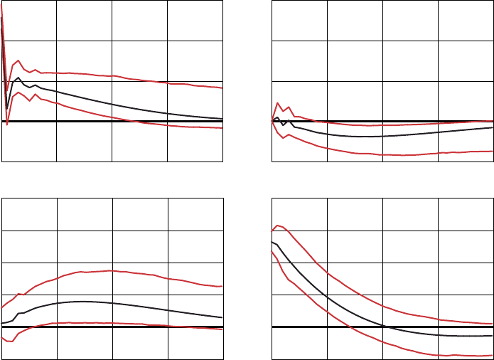
25
Penning- och valutaPolitik 2018:2
-0.2
0.0
0.2
0.4
0.6
-0.2
0.0
0.2
0.4
0.6
10 20 30 40 10 20 30 40
Interest payments Primary surplus
-0.3
0.0
0.3
0.6
0.9
1.2
-0.3
0.0
0.3
0.6
0.9
1.2
10 20 30 40 10 20 30 40
Note. Red lines are 90 percent probability bands.
Figure 11. Dynamic responses to shocks in net interest payments and primary surpluses
As a percentage of GDP
InterestSurplus
Whether these esmates recover scal behavior or merely reect scal dynamics created
by the government’s budget identy is an open queson. The evidence is, at best, merely
suggesve of how Swedish scal policy has behaved. The esmates are crude because
they do not account for the fact that variables in the regressions may be determined
simultaneously. Leeper and Li (2016) point out, for example, that regressions of surpluses on
past debt – or, as in Table 6, interest payments on debt – can be seriously biased, depending
on which monetary-scal regime prevailed over the sample. Less crude esmates would
entail jointly esmang policy behavior and private sector behavior as a means of idenfying
the scal rule. Work of this sort ought to be roune in any country that seeks to follow a
well-specied scal target.
7 Subtle ways that monetary policy aects scal
policy
Government debt is like any other asset: its value depends on discounted expected cash
ows. Cash ows associated with government debt are real primary surpluses – the excess
of revenues over expenditures, not including net interest payments on outstanding debt.
Primary surpluses are debt’s cash ows because they provide the real future payments
that back government debt. Real interest rates determine the rate at which surpluses are
discounted.
7.1 Demand for government bonds
Debt valuaon can be understood using basic supply and demand analysis in the bond
market. Start from the government budget identy above, which I repeat here, slightly
rewrien by dividing through by the price level to convert debt and surpluses from krona
into real units of goods

Sweden’S fiScal framework and monetary policy
26
(18)
Q
t
B
t
P
t
+ s
t
=
(1 + ρQ
t
)B
t−1
P
t
We want to know the value of debt outstanding at the beginning of the current period,
period t, which is
(1 + ρQ
t
)B
t−1
P
t
. Already from the le side of this identy, we see that the
higher is the current real primary surplus, s
t
, the higher is the value of inherited debt (holding
xed the value of newly issued debt). But this identy implies the value of outstanding debt
depends on all future primary surpluses as well, which leads to the debt-valuaon equaon
41
(19)
(1 + ρQ
t
)B
t−1
P
t
= E
t
Σ
∞
T=t
q
t,T
s
T
Using this expression in the budget identy in (18) yields
(20)
Q
t
B
t
P
t
= E
t
Σ
∞
T=t+1
q
t,T
s
T
This expression says that the value of debt sold in period t equals the expected (E
t
) sum of
future discounted real primary surpluses beginning in period t + 1. The variables q
t,T
are real
discount factors, which are products of all future one-period real interest rates between
periods t and T, inverted. Suppose the one-period real interest rate between periods t and
t + 1 is 1 + r
t+1
, then the one-period discount factor between those periods is 1/(1 + r
t+1
). The
two-period discount factor between periods t and t + 2, q
t,t+2
, is simply
1
1 + r
t+1
1
1 + r
t+2
, and so
on.
The real interest rate is an intertemporal price. Today’s real rate, 1 + r
t+1
, is the price of
goods today expressed in terms of future goods, so a lower real rate corresponds to goods
today being relavely cheap. In economic models of the sort that many central banks
employ, the real interest rate is the linchpin for the transmission of monetary policy: when
the central bank reduces nominal interest rates, real rates also tend to fall, inducing people
to substute away from demanding goods in the future toward demanding goods today.
But expression (20) reveals another channel through which real interest rates aect the
economy. The real discount factors in this debt-valuaon equaon express goods in the
future (primary surpluses) in terms of goods today to deliver the value of current debt in
units of current goods (Q
t
B
t
/P
t
). A lower path for real interest rates raises the value of future
goods relave to current goods, which increases the real backing – the present value of
surpluses – and, therefore, the value of debt.
The important point is that discount factors mulply – and therefore compound – interest
rates. If the real interest rate is low today – for example, if r
t+1
is negave – then that low
rate aects all future discount factors and can have a large impact on the present value of
surpluses and thereby on the value of outstanding debt. This creates an important channel
through which monetary policy acons can have scal consequences. More persistent and
larger changes in the monetary policy interest rate will translate into bigger scal impacts.
Valuaon equaon (20) emerges from interacons between supply and demand for
government bonds and, as such, it is a condion that holds in equilibrium. Demand for
government bonds, like demand for other saving devices, is the mirror image of demand for
goods and services: the stronger is the desire to save by accumulang assets, the weaker is
the desire to consume by buying goods and services. When the present value of debt’s cash
ows – primary surpluses – is high, debt becomes more aracve and people substute out
of buying goods into buying bonds. This reduces aggregate demand. Bond prices may rise
and/or the overall level of prices in the economy may fall. As the valuaon equaon makes
41 Dependence on the enre future arises because the budget identy holds for all dates t in the future, so the value of debt
issued at t, B
t
, rises with surpluses the next period, s
t+1
, and so on through me.

27
Penning- och valutaPolitik 2018:2
clear, the present value of debt’s cash ows can rise because people expect higher primary
surpluses – through higher taxes or lower expenditures – or because people expect higher
discount factors (that is, lower real interest rates).
When bond supply is inelasc, expression (20) delivers the demand for nominal bonds in
date t, which may be wrien as
(21) B
d
t
=
1
Q
t
P
t
E
t
PV (S
t+1
)
This demand is readily understood. Demand declines with the price, Q
t
, of bonds, so in
a graph with the price of bonds on the vercal axis, the demand for bonds is downward
sloping, like most demand curves. Because bondholders care about the real value of the
bonds they hold, B
d
t
/P
t
, demand for nominal bonds is homogeneous of degree one in the
price level, just as it is for any nominal asset, such as money. Bond demand also rises with
the real backing for government debt, the expected present value of primary surpluses,
denoted by E
t
PV (S
t+1
), because higher real backing raises the expected stream of payouts to
bond holders.
Figure 12 plots supply and demand for government bonds when the aggregate price level
is on the vercal axis. Vercal supply means bonds are supplied perfectly inelascally. The
inial equilibrium price level is P
1
when the demand schedule is B
d
1
. A lower bond price, lower
expected path of real interest rates (or higher expected path of discount factors), or a higher
expected path of primary surpluses pivots demand to the dashed schedule B
d
2
. At this new
demand curve, bondholders wish to hold more bonds at any given aggregate price level, so
at price level P
1
there is an excess demand for bonds. With an inelasc supply of bonds, the
price level must fall to eliminate the excess demand for nominal bonds. A lower price level
increases the real market value of debt.
Figure 12. Bond market equilibrium
Supply, B
s
, is inelasc and demand is B
d
t
= (P
t
/Q
t
)E
t
PV (S
t+1
)
B
d
1
B
d
2
B
t
B
B
s
P
t
P
1
P
2
This reasoning can be understood in terms of the impacts on aggregate demand. An increase
in demand for bonds is the mirror image of a decrease in demand for goods and services.
When government bonds become more desirable, people reduce their purchases of goods
and services in order to increase their bond holdings. That decrease in goods demand is a
decline in aggregate demand, which drives down the price level, as Figure 12 depicts.
7.2 Applying this reasoning to Sweden
How is any of this relevant for Sweden? Secon 4 reviewed that Swedish government bond
yields have now been negave for more than two years. At mes, those negave yields have
applied to bonds that do not come due for ve years. Table 7 reports a variety of measures
of short-term real interest rates in Sweden over three recent periods. Since January 2008,
nearly all measures have been negave on average. But over the past two and a half

Sweden’S fiScal framework and monetary policy
28
years, the measures have been strongly negave, well over −1.50 percent in some cases.
In contrast, over the seven years before the nancial crisis, real interest rates were around
posive 1.50 percent. Evidently, Sweden is entrenched in a low-interest rate environment.
Low interest rates have been a worldwide phenomenon in recent years. But one clear
reason that Swedish real rates have turned sharply negave is the Riksbank’s policy stance, a
stance that includes negave policy interest rates. Because negave real interest rates imply
real discount factors greater than 1, negave rates have important scal consequences.
Those consequences can be understood through the lens of the debt valuaon equaon in
(20) and the supply-demand graph in Figure 12.
Table 7. Average real interest rates
Real interest rates are computed as the nominal interest rate in the
current month minus the actual inaon rate in the future
Average real interest rates
Repo 3-month treasury
Jan 2001–Dec 2007
CPI 1.41 1.46
CPI-F 1.22 1.29
Core CPI 1.56 1.63
Jan 2001–Aug 2017
CPI 0.55 0.75
CPI-F 0.23 0.44
Core CPI 0.40 0.60
Jan 2008–Aug 2017
CPI −0.08 0.23
CPI-F −0.48 −0.19
Core CPI −0.45 −0.16
Jan 2015–Aug 2017
CPI −1.26 −0.94
CPI-F −1.79 −1.48
Core CPI −1.85 −1.54
Note. For the repo rate, future inaon is next month’s rate. For the 3-month treasury rate, future inaon is the average of
the next three months. Real rates computed using the 3-month Treasury end in June 2017. The 3-month rate is esmated by the
Riksbank using zero-coupon bond yields and a term structure model.
Sources: Sveriges Riksbank, Swedish Naonal Stascal Oce, and author's calculaons
Monetary policy acons are closely linked to bond prices: as interest rates decline,
bond prices and the nominal value of outstanding debt rise. Figure 13 plots the ‘price’
of government bonds (le axis) against the repo rate (right axis). The ‘price’ of bonds is
calculated as the rao of the market value of government bonds to the par value and
is a measure of the Q
t
variable that appears in the equaons.
42
There is a clear negave
relaonship between bond prices and the Riksbank’s policy interest rate, just as theory
would predict. Focusing on the last few years, bond prices rose sharply as the repo rate
headed toward negave territory. Since the repo rate turned negave, bond prices have
remained elevated.
42 This is an approximaon to the krona price of the government’s outstanding bond porolio.

29
Penning- och valutaPolitik 2018:2
1.04
1.06
1.08
1.10
1.12
1.14
1.16
1.18
1.20
2001-11 2003-11 2005-11 2007-11 2009-11 2011-11 2013-11 2015-11
Figure 13. ‘Price’ of government bonds and the repo rate
Market value/par value government debt (le axis) Repo rate (right axis)
-2
-1
0
1
2
3
4
5
6
Negave real interest rates, as in Table 7, beget high real discount rates. Holding the
expected path of primary surpluses xed, higher discount rates raise the current value of
those surpluses to shi out the demand for government bonds, as Figure 12 depicts. As
people substute out of buying goods and services and into buying bonds, the aggregate
price level declines, either now or in the future.
Through the debt-valuaon relaon alone, lower real interest rates exert some direct
deaonary pressures on the economy. Deaonary pressures work against the Riksbank’s
aim to use negave policy interest rates to raise inaon. To support the Riksbank’s
acons, scal policy can eliminate these deaonary pressures by making government
bonds less desirable. Bonds lose their appeal when their real backing – future primary
surpluses – declines. In terms of Figure 12, a lower path for surpluses would oset the eects
of lower real interest rates to pivot the B
d
2
demand schedule le toward its inial posion, B
d
1
.
Swedish scal policy during the negave policy interest rate period has not aimed to
oset the impacts of low interest rates on the desirability of government debt. Instead, net
lending as a percentage of GDP has moved from −1.6 percent in 2014 to 1.2 percent over
2016 and the rst two quarters of 2017. To the extent that this shi in net lending raises the
path of surpluses that people expect, this scal policy makes government debt sll more
aracve, amplifying the deaonary pressures and reducing the Riksbank’s eecveness to
raise inaon.
Recently in Sweden, both monetary and scal policy have increased the desirability and
value of government bonds. Policies have shied the demand curve down, as in Figure 12, to
create deaonary pressures through the bond market. This may help to explain Sweden’s
chronically low inaon rates and why it has been so dicult for the Riksbank to return
inaon to its two percent target.

Sweden’S fiScal framework and monetary policy
30
8 Concluding remarks
The arcle has pointed to types of analysis that are not commonly undertaken by either
monetary or scal authories, but may shed light on how those policies are aecng the
economy. For example, many central banks esmate or calibrate interest-rate rules, which
are used in policy analyses to provide informaon on how actual policy choices compare to
some useful benchmarks. To my knowledge, such exercises are not typically conducted as an
input to scal decisions. As I argued elsewhere, there is much that can be done to improve
the quality of scal analysis in ministries of nances.
43
This arcle does not deny the value of explicit targets for monetary and scal authories
to achieve. It also does not deny the potenal value of monetary and scal rules. The arcle’s
thesis is that these targets and rules should not be designed in isolaon. If monetary and
scal acons are not mutually consistent in ways that this paper has explained, it may be
impossible for the central bank and the government to achieve their objecves.
The arcle’s examinaon of Swedish macroeconomic policies raises some concerns about
whether scal policy is compable with monetary policy’s pursuit of an inaon target. I am
concerned that in recent years the desire to hit a one percent net-lending target conicts
with the Riksbank’s eorts to hit its two percent inaon target. Because these two targets
and any operaonal rules for achieving the targets have been chosen independently of each
other, the potenal for conict is real.
43 Leeper (2011).
31
Penning- och valutaPolitik 2018:2
References
Bai, Y. and E. M. Leeper (2017), ‘Fiscal Stabilizaon vs. Passivity’, Economics Leers, Vol. 154,
pp. 105– 108.
Balke, N. and R. J. Gordon (1986), ‘Appendix B: Historical Data’, in The American Business Cycle:
Connuity and Change, ed. by R. J. Gordon, Chicago: University of Chicago Press, pp. 781–850.
Benhabib, J., S. Schmi-Grohé, and M. Uribe (2002), ‘Avoiding Liquidity Traps’, Journal of Polical
Economy, Vol. 110, pp. 535–563.
Bhaarai, S., J. W. Lee, and W. Y. Park (2016), ‘Policy Regimes, Policy Shis, and U.S. Business Cycles’,
Review of Economics and Stascs, Vol. 98, pp. 968–983.
Bianchi, F. and C. Ilut (2017), ‘Monetary/Fiscal PolicyMix and Agents’ Beliefs’, Review of Economic
Dynamics, Vol. 26, pp. 113–139.
Bodmer, F. (2006), ‘The Swiss Debt Brake: How it Works and What Can Go Wrong’, Schweizerische
Zeitschri für Volkswirtscha und Stask, Vol. 142, pp. 307–330.
Caballero, R. J., E. Farhi, and P.-O. Gourinchas (2017), ‘The Safe Assets Shortage Conundrum’, Journal of
Economic Perspecves, Vol. 31, pp. 29–46.
Clarida, R., J. Galí, and M. Gertler (2000), ‘Monetary Policy Rules and Macroeconomic Stability:
Evidence and Some Theory’, Quarterly Journal of Economics, Vol. 115, pp. 147–180.
Cochrane, J. H. (1999), ‘A Friconless View of U.S. Inaon’, in NBER Macroeconomics Annual 1998, ed.
by B. S. Bernanke and J. J. Rotemberg, Cambridge, MA: MIT Press, Vol. 13, pp. 323–384.
___ (2011), ‘Determinacy and Idencaon with Taylor Rules’, Journal of Polical Economy, Vol. 119,
pp. 565–615.
Danninger, S. (2002), ‘A New Rule: “The Swiss Debt Brake”’, IMF Working Paper WP/02/18, January.
Davig, T. and E. M. Leeper (2006), ‘Fluctuang Macro Policies and the Fiscal Theory’, in NBER
Macroeconomics Annual 2006, ed. by D. Acemoglu, K. Rogo, and M.Woodford, Cambridge: MIT Press,
Vol. 21, pp. 247–298.
___ (2011), ‘Monetary-Fiscal Policy Interacons and Fiscal Smulus’, European Economic Review,
Vol. 55, pp. 211–227.
Erceg, C. J. and J. Lindé (2014), ‘Is There a Fiscal Free Lunch in a Liquidity Trap?’ Journal of the European
Economic Associaon, Vol. 12, pp. 73–107.
Friedman, M. and A. J. Schwartz (1963), A Monetary History of the United States, 1867-1960, Princeton,
NJ: Princeton University Press.
Hall, G. J. and T. J. Sargent (2015), ‘A History of U.S. Debt Limits’, Manuscript, New York University,
December 8.
Internaonal Monetary Fund (2016), ‘Japan Sta Report for the 2016 Arcle IV Consultaon’, July 13.
Jacobson, M. M., E. M. Leeper, and B. Preston (2017), ‘Recovery of 1933’, Manuscript, Indiana
University, February.
Jalil, A. J. and G. Rua (2017), ‘Inaon Expectaons in the U.S. in Fall 1933’, in Research in Economic
History, ed. by S. Wolco and C. Hanes, Emerald Group Publishing Limited, Vol. 33, pp. 139–169.
Johnson, Jr., G. G. (1939), The Treasury and Monetary Policy, 1933–1938, New York: Russell & Russell.
Leeper, E. M. (1991), ‘Equilibria under “Acve” and “Passive” Monetary and Fiscal Policies’, Journal of
Monetary Economics, Vol. 27, pp. 129–147.
___ (2011), ‘Monetary Science, Fiscal Alchemy’, in Macroeconomic Challenges: The Decade Ahead,
2010 Jackson Hole Symposium: Federal Reserve Bank of Kansas City Economic Conference Proceedings,
pp. 361–434.
Sweden’S fiScal framework and monetary policy
32
___ (2016), ‘Why Central Banks Should Care About Fiscal Rules’, Sveriges Riksbank Economic Review,
Vol. 3, pp. 109–125.
___(2017), ‘Fiscal Analysis is Darned Hard’, in Rethinking Fiscal Policy Aer the Crisis, ed. by Ludovít
Ódor, Cambridge, U.K.: Cambridge University Press, pp. 23–70.
Leeper, E. M. and C. Leith (2017), ‘Understanding Inaon as a Joint Monetary-Fiscal Phenomenon’,
in Handbook of Macroeconomics, ed. by J. B. Taylor and H. Uhlig, Amsterdam: Elsevier Press, Vol. 2B,
pp. 2305–2416.
Leeper, E. M. and B. Li (2016), ‘On the Bias in Esmates of Fiscal Policy Behavior’, Manuscript, Indiana
University, October.
Leeper, E. M., N. Traum, and T. B. Walker (2017), ‘Clearing Up the Fiscal Mulplier Morass’, American
Economic Review, Vol. 107, pp. 2409–2454.
Leeper, E. M. and T. B. Walker (2013), ‘Percepons and Mispercepons of Fiscal Inaon’, in Fiscal
Policy aer the Financial Crisis, ed. by A. Alesina and F. Giavazzi, Chicago: University of Chicago Press,
pp. 255–299.
Leeper, E. M. and X. Zhou (2013), ‘Inaon’s Role in Opmal Monetary-Fiscal Policy’, NBER Working
Paper No. 19686, November.
Lubik, T. A. and F. Schoreide (2004), ‘Tesng for Indeterminacy: An Applicaon to U.S. Monetary
Policy’, American Economic Review, Vol. 94, pp. 190–217.
Obseld, M. and K. Rogo (1983), ‘Speculave Hyperinaons in Maximizing Models: Can We Rule
Them Out?’ Journal of Polical Economy, Vol. 91, pp. 675–687.
Phillips, A. W. (1954), ‘Stabilisaon Policy in a Closed Economy’, The Economic Journal, Vol. 64,
pp. 290–323.
Riksgälden Swedish Naonal Debt Oce (2017), ‘Central Government Debt Management: Proposed
Guidelines 2018–2021’, Reg. no 2017/781, 29 September.
Romer, C. D. (1992), ‘What Ended the Great Depression?’ Journal of Economic History, Vol. 52,
pp. 757–784.
Roosevelt, F. D. (1933a), ‘Fireside Chat’, October 22, 1933. Online by Gerhard Peters and John T.
Woolley, The American Presidency Project. hp://www.presidency.ucsb.edu/ws/?pid=14537.
___(1933b), ‘Wireless to the London Conference’, July 3, 1933. Online by Gerhard Peters and John T.
Woolley, The American Presidency Project. hp://www.presidency.ucsb.edu/ws/?pid=14679.
___ (1936), ‘Acceptance Speech for the Renominaon for the Presidency’, Philadelphia, PA, June 27.
Online by Gerhard Peters and John T. Woolley, The American Presidency Project. hp://www.
presidency.ucsb.edu/ws/?pid=15314.
Schaechter, A., T. Kinda, N. Bundina, and A. Weber (2012), ‘Fiscal Rules in Response to the
Crisis – Toward the ‘Next-Generaon’ Rules. A New Dataset’, IMF Working Paper No. WP/12/187, July.
Sims, C. A. (1994), ‘A Simple Model for Study of the Determinaon of the Price Level and the Interacon
of Monetary and Fiscal Policy’, Economic Theory, Vol. 4, pp. 381–399.
___ (2013), ‘Paper Money’, American Economic Review, Vol. 103, pp. 563–584.
___ (2014), ‘Inaon, Inaon Fears, and Public Debt’, Lindau Nobel Laureate Meengs, August 19.
___ (2016), ‘Luncheon Address: Fiscal Policy, Monetary Policy and Central Bank Independence’, in
Designing Resilient Monetary Policy Frameworks for the Future, 2016 Jackson Hole Symposium: Federal
Reserve Bank of Kansas City Economic Conference Proceedings, pp. 313–325.
Sims, C. A. and T. Zha (1998), ‘Bayesian Methods for Dynamic Mulvariate Models’, Internaonal
Economic Review, Vol. 39, pp. 949–968.
Sveriges Riksbank (2018), Monetary Policy Report, Stockholm, April: Sveriges Riksbank.
Swedish Government (2011), The Swedish Fiscal Policy Framework, Stockholm: Regeringskansliet.
33
Penning- och valutaPolitik 2018:2
Taylor, J. B. (1993), ‘Discreon versus Policy Rules in Pracce’, Carnegie-Rochester Conference Series on
Public Policy, Vol. 39, pp. 195–214.
___ (1999), ‘An Historical Analysis of Monetary Policy Rules’, in Monetary Policy Rules, ed. by J. B.
Taylor, Chicago: University of Chicago Press, pp. 319–341.
Tobin, J. (1980), Asset Accumulaon and Economic Acvity, Chicago: University of Chicago Press.
Wallace, N. (1981), ‘A Modigliani-Miller Theorem for Open-Market Operaons’, American Economic
Review, Vol. 71, pp. 267–274.
Woodford, M. (1995), ‘Price-Level Determinacy without Control of a Monetary Aggregate’, Carnegie-
Rochester Conference Series on Public Policy, Vol. 43, pp. 1–46.
___ (2003), Interest and Prices: Foundaons of a Theory of Monetary Policy, Princeton, NJ: Princeton
University Press.
