Microsoft Word - intro_to

Introduction to Excel

This material has been reprinted, with permission, from the Excel Tutorial on the TRIO program webpage

of the University of South Dakota.

A series of "screencast" videos covering the basics of using Excel is also available on the Course Resources

webpage. In addition, you can refer to "CPD 152: Financial Analysis with Excel" available on the Course

Resources webpage. If you need additional tutorial assistance on Excel, you can visit the following two

websites:

http://office.microsoft.com/en-001/support/microsoft-office-2003-2007-2010-training-FX010056500.aspx

www.gcflearnfree.org/excel?search=excel

In addition, the Certified General Accountant's Association of Canada (CGA) has a tutorial entitled

"Computer Tutorial 2 (CT2) – Spreadsheets Using Microsoft Excel". This tutorial may be purchased from

the CGA website. This tutorial provides additional explanations on Excel’s basic functions for financial

purposes, regression analysis, scenario analysis, and charts. CGA website:

www.cga-international.org/become_a_cga/get_started/computer_integration.aspx

Introduction to Spreadsheets

A spreadsheet is the computer equivalent of a paper ledger sheet. It consists of a grid made from columns

and rows. It is an environment that can make number manipulation easy and somewhat painless.

The math that goes on behind the scenes on the paper ledger can be overwhelming. If you change the loan

amount, you will have to start the math all over again (from scratch). But let's take a closer look at the

computer version.

The above two ledgers seem pretty evenly matched. Right? Wrong! The nice thing about using a computer

and spreadsheet is that you can experiment with numbers without having to redo all the calculations. Let's

change the interest rate and then the number of months. Let the computer do the calculations! Once we have

the formulas setup, we can change the variables that are used in the formula and watch the changes.

Change the Interest Rate Change the Number of Months

If you are doing this on paper, you will have to get your calculator back out, grab an eraser and hope you

punched all the right keys and in the right order. A benefit of spreadsheets is that calculations are instantly

updated if one of the referenced entries is changed.

Spreadsheets can be very valuable tools in business. They are often used to play out a series of what-if

scenarios (much like our car purchase here).

Spreadsheet Components

So let's get started digging into what makes a spreadsheet work. Spreadsheets are made up of:



columns



rows



cells (the intersections of columns and rows).

In each cell there may be the following types of data:



text labels: used to describe data



number data (constants): used in calculations



formulas: mathematical equations that utilize data to produce results

In a spreadsheet the Column is defined as the vertical space that is going up and down the window. Letters

are used to designate each Column's location.

In the diagram to the left, Column C is highlighted.

The Row is defined as the horizontal space that is going across the window. Numbers are used to designate

each Row's location.

In the diagram to the left, Row 4 is highlighted.

The Cell is defined as the space where a specified row and column

intersect. Each Cell is assigned a name according to its Column letter

and Row number.

In the diagram to the left, Cell B6 is highlighted. When referencing a cell, you should put the column first

and the row second.

In Excel there are limits to the number of rows and columns in a

sheet…these limits in Excel 2013 are 16,384 columns and

1,048,576 rows. Columns are named from A to Z, then AA,

AB, AC,…, to AZ, BA, BB,…,to ZZ, then AAA, AAB,… , to

XFD. So the top leftmost cell is named A1 and the bottom rightmost cell (should you have that much data) is

named XFD1048576. That is 17,179,869,184 cells (2

Types of Data

There are three basic types of data that can be entered in a spreadsheet:



labels – (text with no numerical value)



constants – (just a number – constant value)



formulas

– (a mathematical equation used to calculate)

Data types Examples Descriptions

LABEL NAME or WAGE or DAYS anything that is just text (could be any combination of

alphanumeric characters usually used for titles or headings)

CONSTANT 5 or 3.75 or -7.4 any number

FORMULA =5+3 or =8*5+3

Mathematical expression – must begin with an equal sign (=)

Labels are text entries. They do not have a value associated with them. We typically use labels to identify

what we are talking about.

In our first example, the labels were:



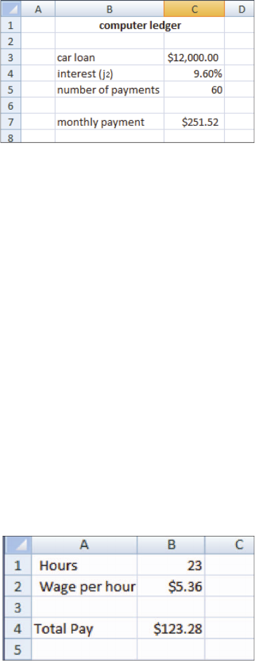
computer ledger



car loan



interest



number of payments



monthly payment

ALL formulas MUST begin with an equal sign (=).

Constants are entries that have a specific fixed value. If someone asks you how old you are, you would

answer with a specific answer. Sure, other people will have different answers, but it is a fixed value for each

person.

In our first example, the constants were:



$12,000



9.6%



As you can see from these examples there may be different types of numbers. Sometimes constants are

referring to dollars, sometimes referring to percentages, and other times referring to a number of items (in

this case 60 months). These are typed into the spreadsheet with just the numbers and are changed to display

their type of number by formatting (we will talk about this later).

Formulas are entries that have an equation that calculates the value to display. We DO NOT type in the

numbers we are looking for; we type in the equation. The results of the equation will be updated upon the

change or entry of any data that is referenced in the equation.

When we are entering formulas into a spreadsheet we want to make as many references as possible to

existing data. If we can reference that information we don't have to type it in again. More importantly, if

that other information changes, we do not have to change the equations.

If you work for 23 hours and make $5.36 an hour, how much do you make?

We can set up this situation using:



three labels



two constants



one equation

Let's look at what could be in cell B4:

= B1 * B2

= 23 * 5.36

$123.28

All three of these choices will produce the same answer, but one is much more useful than the other two.

It is best if we can reference as much data as possible as opposed to typing in the answer or typing data into

equations.

In our last example, things were pretty straightforward. We had number of hours worked multiplied by wage

per hour and we got our total pay. Once you have a working spreadsheet you can save your work and use it

at a later time. If we referenced the actual cells (instead of typing in the answer or data into the equation) we

could update the entire spreadsheet by just typing in the NEW Hours worked. And – you're done!

Let's look at the new spreadsheet:



Hours have been changed to 34



Wage per hour is the same



Total Pay would have to be changed to either

= 34 * 5.36 or $182.24



However, the formula would still be = B1 * B2

If in cell B4 we had typed in either = 23 * 5.36 or $123.28 the first time and just changed the hours worked

here, Total Pay in cell B4 would still be $123.28, and we would have to retype what is in cell B4.

INSTEAD we typed in references to the data that we wanted to use in the equation.

We typed in = B1 * B2. These are the locations of the data that we want to use in our equation so Excel

recalculates the Total Pay with the new values.

Again, it is best if we can reference as much data as possible as opposed to typing data into equations or

answers into the cell.

Excel Formulas (Functions)

Spreadsheets have many math functions built into them. Of the most basic operations are the standard

multiply, divide, add and subtract. These operations follow the order of operations (just like algebra). Let's

look at some examples.

For these following examples let's consider the following data:

Operation Symbol Constant

Data

Referenced

Data

Answer

Multiplication

* = 5 * 6 = A1 * B3 30

Division

/ = 8 / 4 = A3 / B2 2

Addition

+ = 4 + 7 = B2 + A2 11

Subtraction

- = 8 - 3 = A3 - B1 5

Selecting Cells

Selecting cells is a very important concept of a spreadsheet. We need to know how to reference the data in

other parts of the spreadsheet in order to specify the range of numbers that should be included in a formula

or a graph. When entering your selection you may use the keyboard or the mouse.

We can select several cells together if we can specify a starting cell and a stopping cell. This will select all

the cells within this specified block of cells.

Using the same data as before we will look at various selection methods.

Referring to the table below, if we wanted to add up the group of cells in the "To Add Up" column, you

would insert the respective cell range found in the "Type In" column into the SUM formula, either by typing

or clicking:

=SUM(Type In)

=SUM(Click On)

To Add Up Type In Click On

A1, A2, A3 A1:A3 A1, with button down drag to A3

A1, B1 A1:B1 A1, with button down drag to B1

A1, B3 A1, B3 A1, type in comma, B3

A1, A2, B1, B2 A1:B2 A1, with button down drag to B2

Common Functions

SUM

Probably the most popular function in any spreadsheet is the SUM function. The SUM function takes all of

the values in each of the specified cells and totals their values. The syntax is:

=SUM(first value, second value, …)

In the first and second spots you can enter any of the following (constant, cell, range of cells).



Blank cells will return a value of zero to be added to the total.



Text cells cannot be added to a number and will produce an error.

Notice that in A4 there is a TEXT entry. This has NO numeric value and cannot be included in a total or it

will result in an error.

Example Cells to SUM Answer

=sum (A1:A3) A1, A2, A3 150

=sum (A1:A3, 100) A1, A2, A3, 100 250

=sum (A1 + A4) A1, A4 #VALUE!

=sum (A1:A2, A5) A1, A2, A5 75

AVERAGE (MEAN)

The AVERAGE function finds the arithmetic mean of the specified data. This is found by adding all of the

indicated cells together and dividing by the total number of cells. The syntax is as follows:

=AVERAGE(first value, second value, …)

Text fields and blank entries are not included in the calculations of the Average function.

Example Cells to AVERAGE Answer

=average (A1:A4) A1, A2, A3, A4 62.5

=average (A1:A4, 300) A1, A2, A3, A4, 300 110

=average (A1:A5) A1, A2, A3, A4, A5 62.5

=average (A1:A2, A4) A1, A2, A4 58.33

MAXIMUM

The next function we will discuss is MAX (Maximum). This will return the greatest (maximum) value in the

selected range of cells. The syntax is as follows:

=MAX(first value, second value, …)

Text fields and blank entries are not included in the calculations of the MAX Function.

Example of Max Cells to Look At Answer

=max (A1:A4) A1, A2, A3, A4 30

=max (A1:A4, 100) A1, A2, A3, A4, 100 100

=max (A1,A3) A1, A3 30

=max (A1, A5) A1, A5 10

MINIMUM

The next function we will discuss is MIN (Minimum). This will return the lowest (minimum) value in the

selected range of cells. The syntax is as follows:

=MIN(first value, second value,)

Text fields and blank entries are not included in the calculations of the MIN Function.

Example of Min Cells to Look At Answer

=min (A1:A4) A1, A2, A3, A4 10

=min (A2:A3, 100) A2, A3, 100 20

=min (A1,A3) A1, A3 10

=min (A1, A5) A1, A5 (displays the least

number)

Notice that there is no Range function in Excel. To find out the range of a sample, simply subtract the

maximum value from the minimum value of the sample (try to do it by typing in an equation that will

reference your Max and Min cell values).

PAYMENT

(introducing the concept of equivalent interest rates within the context of a Canadian Mortgage)

The PMT function in Excel calculates the monthly payment for a loan given the periodic interest rate, the

number of periods to pay off the loan, and the amount of the loan.

The formula for the PMT function is

=PMT(rate,nper,pv,fv,type)

where:

 Rate represents the periodic interest rate for the loan

 NPER represents the total number of payments in the loan

 PV represents the principal or present value (negative value if you owe the money)

 FV represents the future value

 Type represents when the payments are due (0 = at the end of the period or omitted, 1 = at the

beginning of the period)

NOTE: If you are not given a FV or Type (as in this question) you can omit them from your function.

Note the solution was NOT typed into the cell C7. A formula was typed into that cell; the formula that was

typed into the spreadsheet was:

=PMT(C9,C5,-C3)

We now introduce the concept of equivalent interest rates as they are the basis to another type of annuity, the

mortgage. The interest rate offered by Canadian Institutions are quoted as a per annum rate, compounded

semi-annually, denoted j

2, with monthly payments. Since the contract rate is compounded semi-annually and

the payments are monthly, the interest rate must be converted and expressed as an equivalent nominal rate

with monthly compounding.

Consider the example where the interest rate of 9.6% is compounded semi-annually, that is, the interest rate

given is semi-annual, while the payment period is monthly. In order to find the periodic rate for the PMT

function we have to first convert the interest rate to its effective (annual) rate, then convert it to its nominal

interest rate with monthly compounding and finally divide by 12 to find the periodic rate. That is, we have

to convert the j2 rate to the j12 rate, and then divide by 12 to find the periodic rate i.

With a financial calculator the steps are:

Press Display Comments

9.6  NOM%

9.6

2  P/YR

 EFF%

9.8304

12  P/YR

 NOM%

9.413447

÷ 12 = .784454

Equivalent Interest Rates

Two interest rates are equivalent if, for the same amount borrowed, over the same period of time,

the same amount is owed at the end of the period.

The nominal interest rate is an interest rate quoted as a rate per annum. The nominal rate is represented

mathematically as "j

" where:

= nominal interest rate compounded "m" times per year

m = number of compounding periods per annum

i = interest rate per compounding period

The periodic interest rate represents the interest rate per compounding period. The nominal rate of interest

compounded "m" times per year (j

) is equal to the periodic interest rate per compounding period (i) times

the number of compounding periods per year (m).

j = i × m

The effective interest rate is a nominal interest rate with yearly compounding. The effective rate is used to

standardize interest rates to allow borrowers and lenders to compare different rates on a common basis.

Alternatively, you can use Excel to find the periodic rate:

It is also important to type in the reference cells for the constants instead of the constants. Had I entered

=PMT(.096,60,-12000) my formula would only work for that particular set of data. I could change the

months above and the payment would not change.

 Remember to enter the cell where the data is stored and NOT the data itself.

 Formulas OR Functions MUST BEGIN with an equal sign (=).

Again, we use formulas to calculate a value to be displayed.

IF FUNCTION

The IF function returns one value if a condition you specify is TRUE, and another value if that condition is

FALSE. The formula is formatted as follows: =IF(logical_test, [value if true], [value if false]). Any value

or expression that can be evaluated as either TRUE of FALSE can be placed in the logical test section. The

most common logical tests are greater than (>), less than (<), or equal (=).

Examples of IF Cells to Look At Answer

=IF(A1>100,"Over 100","Under 100") A1 Under 100

=IF(A2>100,"Over 100","Under 100") A2 Over 100

=IF(A3+A1>100,"Over 100","Under 100") A3, A1 Over 100

=IF(A4-A2>100,"Over 100","Under 100") A4, A2 Under 100

NET PRESENT VALUE

Net present value (NPV) is one of the financial functions in Excel. To calculate an NPV at a discount rate of

20%, perform the following steps:

 Select the Formulas tab, then click Insert Function;

 Select Financial from the drop-down list, scroll down, then double-click on NPV;

 The NPV program will have the following arguments:

Rate 20%

Value 1 Initial cost (a negative)

Value 2…Value N

Subsequent periodic net cash flows

Tip: rather than filling in each individual value, you can place the cursor in the text box beside Value 2 and

then use the mouse to select all of the individual cash flows.

The NPV function will then compute the net present value, a dollar figure representing the present value of

benefits less the present value of costs. If the NPV is positive, then the return on the investment is 20% or

greater, given the cash flows indicated. If the NPV is negative, then the return on the investment is less than

20%.

NOTE: The steps shown for calculating the net present value of cash flows in Microsoft Excel assume that

the initial cost of investment is incurred at the end of Year 1. This is due to the default assumption in most

spreadsheet programs, including Excel, that cash flows are received or paid at the end of each period.

However, this may not be realistic, as the initial cost for an investment is more typically paid at the

beginning of Year 1 (sometimes called Year 0).

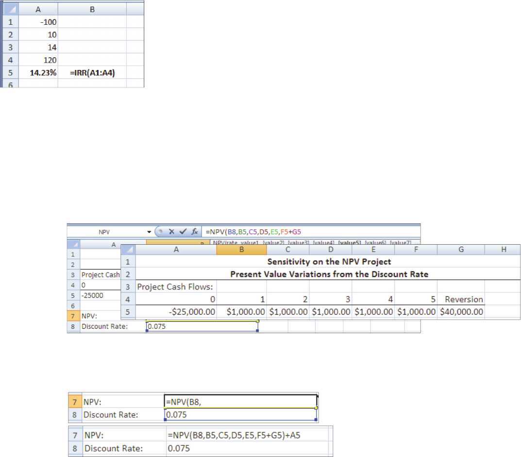
For example, assume you have an investment that costs you $100 today, and pays you $10 in one year, $14

in two years, and then $120 in three years. The discount rate is 10%. If you use the NPV function in Excel,

the formula is as follows: =NPV(B9,B4:B7) yielding a NPV of $9.84. This is calculated assuming that the

$100 was spent at the end of Year 1 and $10 was received at the end of Year 2, which is not correct since

the $100 was actually spent at the beginning of year 1 and $10 was received at the end of Year 1. This

problem can be corrected by using the NPV function to calculate the present value of all cash flows from the

end of Year 1 on, and then manually adding the initial cost. In Excel, the general formula is as follows:

=NPV(rate,CF

1:CFN)+CF0.

For our example, the formula will look as follows: =NPV(B9,B5:B7)+B4. The calculated NPV is now

$10.82, which is the same as the value calculated using the HP10BII/10BII+ business calculator.

It is worth noting that the IRR function in Excel already takes this initial cost issue into account and

correctly calculates the Internal Rate of Return (discussed in the next section). In this case, the IRR is

14.23%.

INTERNAL RATE OF RETURN

Internal Rate of Return (IRR) is another important financial function in Excel. Where NPV calculates the

present value dollar return given a discount rate, IRR will calculate the precise return on capital. To

calculate an IRR, perform the following steps:

 Select the Formulas tab, then click Insert Function;

 Select Financial from the drop-down list, scroll down, then double-click on IRR;

 The IRR program will have the following instructions:

Values Initial cost (negative) and subsequent periodic net cash flows

Guess 0.2 (rough estimate of IRR, to give software a starting point for its calculation)

Tip: rather than filling in each individual value, you can place the cursor in the Values blank space and then

use the mouse to highlight all of the series of individual cash flows.

The IRR is expressed as percentage.

WHAT-IF ANALYSIS

(Note: Do not confuse with IF function)

Excel allows you to perform a basic sensitivity analysis of a change in a variable. The What-If analysis is a

built in function that allows you to see the effect of a change in a key variable on a given outcome. In this

example we will be using an NPV formula and changing the discount

rate to see the varying outcomes (changes in NPV).

1. Set up the project's cash flows at the top of the page. Make

sure to carefully enter positive or negative cash flows in each cell of

the timeline. In this example the reversion is the sale price of the

project.

2. Create a dedicated cell for the discount rate (B8).



Enter your NPV formula - type the equal sign followed by NPV and the open bracket.



Then select the cell in which you have the discount rate (B8) followed by a comma.



Next select each of your cash flow cells starting with period one (B5). Separate each entry

with a comma. Note that the cash flow at period 5 is actually the sum of the $1,000 cash

flow (F5) and the $40,000 reversion price (G5). This is because both occur at the same

point in time.



Close the brackets after the final year's cash flow.



Add in the cash flow occurring at time zero (A5).



Press the enter key. You will notice that the cell now contains the NPV of the cash flows

using a discount rate of 0.075.

3. Now it is time to construct the What-If worksheet.

 Enter the desired discount rates in a column, these will be the different rates used to test the

NPV. Make sure the first cell in the worksheet corresponds to the rate that you used for

your initial NPV calculation.

 In the cell to the right of the first value (B12) you will need to set it equal to the NPV

formula. Click on the cell (B12) and press the = key, then click on the cell that contains the

NPV formula (B7) and press the enter key. It should appear as the figure below:

 Now select the range of discount rates and the range of NPV values that you want to fill.

Do this by clicking and dragging the mouse from the top left value to the bottom right value

you want to select.

 At the toolbar at the top of the page, navigate to the Data tab.

 Click on the What-If Analysis button and then on the Data Table option from the drop down

menu.

 A dialogue box will pop up on the screen. In the "Column input cell" dialogue box enter the

location of the cell that held the original discount rate used in the NPV formula. In our

example it is B8. The value can be entered in two ways, either by manually typing in $B$8

in the dialog box or by clicking on the discount rate cell.

 Click on the OK button and the table will be filled with different NPV values/outcomes for

each corresponding discount rate.

The result of our sensitivity analysis is displayed above. Changing any cash flow value will automatically

update the table.

GOAL SEEK FUNCTION

The Goal Seek function of Excel allows for a variable to be changed until the different outcomes match a

defined outcome. We will now use it to solve for an NPV of zero, also known as the IRR. We will continue

from the last example of creating a What-If worksheet.

1. Navigate to the Data tab found on the toolbar at the top of the page.

2. Click on the What-If Analysis button and then on the Goal Seek option from the drop down menu.

3. A dialogue box will appear on the screen. Place the cursor in the "Set cell" dialogue box and click

on the cell containing the NPV formula (B7). Enter a value of zero in the "To value" dialogue box.

Place the cursor in the "By changing cell" dialogue box and select the cell containing the discount

rate (B8).

4. Click OK and OK again. Excel will change the NPV to zero and a new discount rate will be

displayed.

In this example we used Goal Seek to find a discount rate that resulted in an NPV of zero. While some

might notice that this can also be achieved by using Excel's IRR function, the Goal Seek function allows the

user to look for any target NPV.

Accessing all the Functions

While it is possible to type in every function in the keyboard, in Excel there is a help tool for functions

called the Insert Function which will initiate the Function Wizard.

There are three ways to access the function wizard:

1. If you look at the Standard Toolbar, the function wizard icon looks like . Clicking on the icon

will open the Insert Function window.

2. Go to the Formulas tab, then Insert Function.

3. When you type in the "=" sign in a cell in order to start a formula, a menu of the most recent

functions used is available on the left.

Click on the arrow pointing down in order to open the menu and choose the function you want to use. If the

function that you need does not appear on the pull down menu, click on "More Functions..." and the Insert

Function window will appear.

The Insert Function window appears with the function

categories in a drop-down text box near the top with

choices (such as Most Recently Used, All, Financial,

and Statistical) and the functions in each category

listed in the window below. U pon choosing the

function and clicking OK, Excel will open a new

window (Function Arguments) where you will input

the data or cells or range of cells needed to complete

the function.

Mini descriptions are available for each of the

functions. It is often necessary for you to understand

the functions in order to be able to figure out these

descriptions. In the window below, many functions

needed to complete a statistics project are listed. You

can access all of these functions by choosing the

"Statistical" category and looking for the function

name in the menu. Make sure that you choose the appropriate function! Many of the functions look similar,

but have different properties (example: STDEV, STDEVA, STDEVP, STDEVPA). Read the brief

description at the bottom of the window. Most of the time, you will be using the first type of the function

listed (i.e. STDEV not

STDEVA, STDEVP, not STDEVPA).

Some statistical measures do not have a corresponding function. For example, to calculate the Coefficient of

Variation you will need to use the Excel functions to calculate the mean and the standard deviation and then

use the Coefficient of Variation formula to calculate the statistic.

Copying Formulas: Absolute and Relative Positioning

Sometimes when we enter a formula, we need to repeat the same formula for many different cells. In the

spreadsheet we can use the copy and paste command. The cell locations in the formula are pasted and any

references changed relative to the position we COPY them from.

For example, if the original cell (C1) had the equation (=A1+B1), when we copy and paste the function it

will look to the two cells to the left. So the equation pasted into (C2) would be (=A2+B2). The equation

pasted into (C3) would be (=A3+B3); the equation pasted into (C4) would be (=A4+B4); and so on.

Often we have several cells that need the same formula (in relationship) to the location it is to be typed into.

There is a short cut that is called Fill Down. There are a number of

ways to perform this operation. Here are the two most common

methods:

Method 1:

1. select the cell that has the original formula

2. hold the shift key down and click on the last cell (in the series that needs the formula)

3. go to the "Home" tab, "Editing" group, "Fill", then "Down")

Method 2:

1. select the cell that has the original formula

2. hold your mouse on the dot on the right bottom corner of the cell

3. without releasing your mouse drag the cursor down to the last cell (in the series that needs the

formula)

4. release the mouse

Sometimes when you are copying a formula, it is necessary to keep a certain position that is not relative to

the new cell location. For example, if you are producing an amortization table, you would want all the cells

that calculate the payment to refer to a single set of data (i.e., the term or the interest rate) contained in one

or more fixed cells. This is possible by inserting a $ before the Column letter and/or a $ before the Row

number. This is called Absolute Referencing.

Following our example, if we were to fill down with this formula we would have the exact same formula in

all of the cells C1, C2, C3, and C4. The dollar signs lock the cell location to a FIXED position. When it is

copied and pasted it remains exactly the same (not relative).

We can also fill right. We must select the original cell (and the cells to the right) and select from the Edit

menu–Fill and Right (Excel 2007: "Home" tab, "Editing" group, "Fill", then "Right").

If we were to fill right from A1 to C1 we would get the formulas displayed in the table below. Notice that

the second part of the equation is FIXED or ABSOLUTE REFERENCE, so always reference B3 which is

10.

Answers across Row 1 would be A1=16, B1=12, C1=15 (below).

Formatting

Spreadsheets can be pretty dry, so we need some tools to dress them up a little. We can use most of the

tricks in our word processor to do the formatting of text. We can use things like: bold face, italics,

underline, different colors of both text and cell background, different alignments (left, right, centre), and

changes in font size and font type, as well as setting the number of decimal places.

We need to select the cell (or group of cells) that we wish to change the formatting and then use the "Home"

tab; the "Font" group, "Alignment" group, and "Number" group all have various "quick formats" that you

can use.

A scan across the ribbon shows in the "Font" group the font type and size, bold, italic, underline, borders,

color fill, and text color; in the "Alignment" group vertical and horizontal alignment within cells,

orientation, left and right indent, text wrapping and cell merging; and, in the "Number" group, style,

currency, percentage, and comma formats, as well as increase or decrease the decimal.

If you want more options than those offered on the ribbon, click on the bottom-right corner of any of the

three groups: "Font", "Alignment", or "Number". The following window will be displayed; there are

several options beyond what is available on the ribbon.

As mentioned previously, we can change the format of numbers within cells. This means things like

displaying the appropriate number of decimals, showing currency signs, percentage, even red numerals for

negative dollars. It is best to keep numbers describing similar items as uniform as possible, and the count of

decimal places reasonable…if all of your numbers are in dollars and cents, there is not much point in an

interest rate being 15 decimal places. If we have the number 3.532626246724217, we would probably have

to make the column wider and at the least bore most people. We need to set the number of decimal places to

what is important. If this was a dollar figure that represented a calculated sales tax it should be formatted as

$3.53.

Below is a screen displaying what you would see if you select a cell (or group of cells) and then use the

"Home" tab and click on the bottom-right corner of the "Number" group (or click on the Number tab shown

on the Format Cells window previously). The first screen sample shows the General format (which is the

default) and the second the Number format with choices for a thousands separator, red negative numbers,

and number of decimal places.

A question that everyone who has ever worked on a spreadsheet has asked at one time or another is, "Where

did all my numbers go?" or a similar question, "Where did all of those ####### come from and why are

they in my spreadsheet?"

The problem is that the number trying to be displayed in a particular cell is too wide for the cell to display

properly. To clear up the problem we just need to make the column wider. You can do this many ways.

Here are two ways to change the column width:

1. Select the column (or columns) by clicking on their labels (letters), then on the "Home" tab, "Cells"

group, then "Format". Click Column Width and type in a new number for the column width in the

small window. The selected columns will have a new width. The example below changes the widths

of Columns A, B, and C to 22 (from

8.43).

2. Move the mouse (arrow) to the right side of the column label (see the following figure) and click

and drag the mouse to the right (to make wider) or left (to make smaller). Let up on the mouse

button when the column is wide enough. You could also double click the mouse button between the

column labels. This will automatically resize your column so that it will be large enough to display

the largest number or label in that column.

Notice that the cursor changes to a vertical line

with arrows pointing left and right. In this position

you are set to change the width of Column C.

3. You could also double click the mouse

button between the column labels, as shown in the figure above. This will automatically resize your

column so that it will be large enough to display the largest number or label in that column.

In many spreadsheets you can also change the vertical height of a row by moving the lower edge of the row

title (number).

If you have a spreadsheet designed and you forgot to include some important information, you can insert a

column into an existing spreadsheet. What you must do is click on the column label (letter) and on the

"Home" tab,"Cells" group, "Insert", then "Insert Sheet Columns". This will insert a column immediately

left of the selected column. The following example will insert a new column between the current columns B

and C.

As you can see from this example, there was a blank column inserted into the spreadsheet… a new column

C. The old column C is now column D, the old column D is now column E, and the old column E is now F.

You might wonder if this will affect your referenced formulas. The referenced cells are changed to their new

locations. For example:

C4 =C3+B4

BECOMES C4 =D3+B4

Likewise, we can also insert rows. With the row label (number) selected you must choose the "Insert Sheet

Rows" from the Insert menu. Again, this will insert a row above the row you have selected. The following

example will insert a new row between the current rows 2 and 3.

The old row 3 is now row 4 and the old row 4 is now row 5.

The formulas will be updated to their corresponding locations.

C3 = C2+B3

BECOMES C4 = C2+B4

Multiple Worksheets

Within Excel you can open and use multiple worksheets in one file. At the bottom of the Excel screen there

are three tabs called "Sheet1", "Sheet2" and "Sheet3". You can click on a new tab to start working on a

separate spreadsheet. You can also rename those tabs (ex. Question 1, Question 2 etc.) by right clicking on

the tab and selecting "Rename". Additionally, you can create further worksheets by clicking on the "Insert

Worksheet" tab. When working on one spreadsheet you can link to a cell in another spreadsheet by clicking

on the spreadsheet tab you want to go to, clicking the appropriate cell, and then returning to your original

spreadsheet. NOTE: You should only link to cells within the same excel file, otherwise, when you close the

second file your functions will not work.

Hiding Columns and Rows

Within Excel you can hide columns and rows if you want to simplify your spreadsheet. To hide a column,

right click on the column header (B, for example) and select "Hide". To unhide your column, highlight the

headers to the right and left of your hidden column (A and C, for example) and select "Unhide". The same

applies for hiding and unhiding rows.

Freezing Columns and Rows

In Excel, you can freeze panes to keep specific rows or columns visible when you scroll in the worksheet.

For example, you might want to keep row and column headings visible when you scroll. In order to freeze

rows or columns:

1. On the worksheet, do one of the following:

 To lock rows, select the row below the row or rows that you want to keep visible when you

scroll.

 To lock columns, select the column to the

right of the column or columns that you want

to keep visible when you scroll.

 To lock both rows and columns, click the cell below and to the right of the rows and

columns that you want to keep visible when you scroll. Tip: To cancel a selection of cells,

click any cell on the worksheet

2. On the View tab, in the Window group, click the arrow below Freeze Panes.

3. Do one of the following:

 To lock one row only, click Freeze Top Row.

 To lock one column only, click Freeze First Column.

 To lock more than one row or column, or to lock both rows and columns at the same time,

click Freeze Panes.

To unlock frozen columns or rows go to the View tab, in the Window group, and click Unfreeze Panes

Excel is a great tool! A good understanding of the program will go a long way in helping you prepare for the

Project work required in the course. Knowledge of the Math Review Kit and the use of HP10BII/10BII+

financial calculator are also highly recommended and excellent adjuncts to understanding Excel and the

financial concepts introduced in the course.