
CONCEPTS OF
PROGRAMMING LANGUAGES
TENTH EDITION
This page intentionally left blank

CONCEPTS OF
PROGRAMMING LANGUAGES
TENTH EDITION
ROBERT W. SEBESTA
University of Colorado at Colorado Springs
Boston Columbus Indianapolis New York San Francisco Upper Saddle River
Amsterdam Cape Town Dubai London Madrid Milan Munich Paris Montreal Toronto
Delhi Mexico City Sao Paulo Sydney Hong Kong Seoul Singapore Taipei Tokyo

Vice President and Editorial Director, ECS:
Marcia Horton
Editor in Chief: Michael Hirsch
Executive Editor: Matt Goldstein
Editorial Assistant: Chelsea Kharakozova
Vice President Marketing: Patrice Jones
Marketing Manager: Yez Alayan
Marketing Coordinator: Kathryn Ferranti
Marketing Assistant: Emma Snider
Vice President and Director of Production:
Vince O’Brien
Managing Editor: Jeff Holcomb
Senior Production Project Manager: Marilyn Lloyd
Manufacturing Manager: Nick Sklitsis
Operations Specialist: Lisa McDowell
Cover Designer: Anthony Gemmellaro
Text Designer: Gillian Hall
Cover Image: Mountain near Pisac, Peru;
Photo by author
Media Editor: Dan Sandin
Full-Service Vendor: Laserwords
Project Management: Gillian Hall
Printer/Binder: Courier Westford
Cover Printer: Lehigh-Phoenix Color
This book was composed in InDesign. Basal font is Janson Text. Display font is ITC Franklin Gothic.
Copyright © 2012, 2010, 2008, 2006, 2004 by Pearson Education, Inc., publishing as Addison-Wesley.
All rights reserved. Manufactured in the United States of America. This publication is protected by Copy-
right, and permission should be obtained from the publisher prior to any prohibited reproduction, storage
in a retrieval system, or transmission in any form or by any means, electronic, mechanical, photocopying,
recording, or likewise. To obtain permission(s) to use material from this work, please submit a written
request to Pearson Education, Inc., Permissions Department, One Lake Street, Upper Saddle River, New
Jersey 07458, or you may fax your request to 201-236-3290.
Many of the designations by manufacturers and sellers to distinguish their products are claimed as trade-
marks. Where those designations appear in this book, and the publisher was aware of a trademark claim,
the designations have been printed in initial caps or all caps.
Library of Congress Cataloging-in-Publication Data
Sebesta, Robert W.
Concepts of programming languages / Robert W. Sebesta.—10th ed.
p. cm.
Includes bibliographical references and index.
ISBN 978-0-13-139531-2 (alk. paper)
1. Programming languages (Electronic computers) I. Title.
QA76.7.S43 2009
005.13—dc22 2008055702
10 9 8 7 6 5 4 3 2 1
ISBN 10: 0-13-139531-9
ISBN 13: 978-0-13-139531-2

New
to the
Tenth
Ed
iti
on
Chapter
5: a new
section
on the let
construct
in
functional pro-
gramming languages
was
added
Chapter
6: the
section
on
COBOL's record operations
was
removed;
new
sections
on
lists, tuples,
and
unions
in F#
were added
Chapter
8:
discussions
of
Fortran's
Do
statement
and
Ada's
case
statement were removed; descriptions
of the
control statements
in
functional
programming languages were moved
to
this chapter
from
Chapter
15
Chapter
9: a new
section
on
closures,
a new
section
on
calling sub-
programs indirectly,
and a new
section
on
generic
functions
in F#
were
added;
the
description
of
Ada's
generic subprograms
was
removed
Chapter
11:
a new
section
on
Objective-C
was
added,
the
chapter
was
substantially revised
Chapter
12: a new
section
on
Objective-C
was
added,
five new fig-
ures were added
Chapter
13: a
section
on
concurrency
in
functional programming
languages
was
added;
the
discussion
of
Ada's asynchronous message
passing
was
removed
Chapter
14: a
section
on C#
event handling
was
added
Chapter
15: a new
section
on F# and a new
section
on
support
for
functional
programming
in
primarily imperative languages were added;
discussions
of
several
different
constructs
in
functional programming
languages
were moved
from
Chapter
15
to
earlier chapters

vi
Preface
Changes for the Tenth Edition
T
he goals, overall structure, and approach of this tenth edition of Concepts
of Programming Languages remain the same as those of the nine ear-
lier editions. The principal goals are to introduce the main constructs
of contemporary programming languages and to provide the reader with the
tools necessary for the critical evaluation of existing and future programming
languages. A secondary goal is to prepare the reader for the study of com-
piler design, by providing an in-depth discussion of programming language
structures, presenting a formal method of describing syntax and introducing
approaches to lexical and syntatic analysis.
The tenth edition evolved from the ninth through several different kinds
of changes. To maintain the currency of the material, some of the discussion
of older programming languages has been removed. For example, the descrip-
tion of COBOL’s record operations was removed from Chapter 6 and that of
Fortran’s Do statement was removed from Chapter 8. Likewise, the description
of Ada’s generic subprograms was removed from Chapter 9 and the discussion
of Ada’s asynchronous message passing was removed from Chapter 13.
On the other hand, a section on closures, a section on calling subprograms
indirectly, and a section on generic functions in F# were added to Chapter 9;
sections on Objective-C were added to Chapters 11 and 12; a section on con-
currency in functional programming languages was added to Chapter 13; a
section on C# event handling was added to Chapter 14; a section on F# and
a section on support for functional programming in primarily imperative lan-
guages were added to Chapter 15.
In some cases, material has been moved. For example, several different
discussions of constructs in functional programming languages were moved
from Chapter 15 to earlier chapters. Among these were the descriptions of the
control statements in functional programming languages to Chapter 8 and the
lists and list operations of Scheme and ML to Chapter 6. These moves indicate
a significant shift in the philosophy of the book—in a sense, the mainstreaming
of some of the constructs of functional programming languages. In previous
editions, all discussions of functional programming language constructs were
segregated in Chapter 15.
Chapters 11, 12, and 15 were substantially revised, with five figures being
added to Chapter 12.
Finally, numerous minor changes were made to a large number of sections
of the book, primarily to improve clarity.

The Vision
This book describes the fundamental concepts of programming languages by
discussing the design issues of the various language constructs, examining the
design choices for these constructs in some of the most common languages,
and critically comparing design alternatives.
Any serious study of programming languages requires an examination of
some related topics, among which are formal methods of describing the syntax
and semantics of programming languages, which are covered in Chapter 3.
Also, implementation techniques for various language constructs must be con-
sidered: Lexical and syntax analysis are discussed in Chapter 4, and implemen-
tation of subprogram linkage is covered in Chapter 10. Implementation of
some other language constructs is discussed in various other parts of the book.
The following paragraphs outline the contents of the tenth edition.
Chapter Outlines
Chapter 1 begins with a rationale for studying programming languages. It then
discusses the criteria used for evaluating programming languages and language
constructs. The primary influences on language design, common design trade-
offs, and the basic approaches to implementation are also examined.
Chapter 2 outlines the evolution of most of the important languages dis-
cussed in this book. Although no language is described completely, the origins,
purposes, and contributions of each are discussed. This historical overview is
valuable, because it provides the background necessary to understanding the
practical and theoretical basis for contemporary language design. It also moti-
vates further study of language design and evaluation. In addition, because none
of the remainder of the book depends on Chapter 2, it can be read on its own,
independent of the other chapters.
Chapter 3 describes the primary formal method for describing the syntax
of programming language—BNF. This is followed by a description of attribute
grammars, which describe both the syntax and static semantics of languages.
The difficult task of semantic description is then explored, including brief
introductions to the three most common methods: operational, denotational,
and axiomatic semantics.
Chapter 4 introduces lexical and syntax analysis. This chapter is targeted to
those colleges that no longer require a compiler design course in their curricula.
Like Chapter 2, this chapter stands alone and can be read independently of the
rest of the book.
Chapters 5 through 14 describe in detail the design issues for the primary
constructs of programming languages. In each case, the design choices for several
example languages are presented and evaluated. Specifically, Chapter 5 covers
the many characteristics of variables, Chapter 6 covers data types, and Chapter 7
explains expressions and assignment statements. Chapter 8 describes control
Preface vii

viii Preface
statements, and Chapters 9 and 10 discuss subprograms and their implementa-
tion. Chapter 11 examines data abstraction facilities. Chapter 12 provides an in-
depth discussion of language features that support object-oriented programming
(inheritance and dynamic method binding), Chapter 13 discusses concurrent
program units, and Chapter 14 is about exception handling, along with a brief
discussion of event handling.
The last two chapters (15 and 16) describe two of the most important alterna-
tive programming paradigms: functional programming and logic programming.
However, some of the data structures and control constructs of functional pro-
gramming languages are discussed in Chapters 6 and 8. Chapter 15 presents an
introduction to Scheme, including descriptions of some of its primitive functions,
special forms, and functional forms, as well as some examples of simple func-
tions written in Scheme. Brief introductions to ML, Haskell, and F# are given
to illustrate some different directions in functional language design. Chapter 16
introduces logic programming and the logic programming language, Prolog.
To the Instructor
In the junior-level programming language course at the University of Colorado
at Colorado Springs, the book is used as follows: We typically cover Chapters 1
and 3 in detail, and though students find it interesting and beneficial reading,
Chapter 2 receives little lecture time due to its lack of hard technical content.
Because no material in subsequent chapters depends on Chapter 2, as noted
earlier, it can be skipped entirely, and because we require a course in compiler
design, Chapter 4 is not covered.
Chapters 5 through 9 should be relatively easy for students with extensive
programming experience in C++, Java, or C#. Chapters 10 through 14 are more
challenging and require more detailed lectures.
Chapters 15 and 16 are entirely new to most students at the junior level.
Ideally, language processors for Scheme and Prolog should be available for
students required to learn the material in these chapters. Sufficient material is
included to allow students to dabble with some simple programs.
Undergraduate courses will probably not be able to cover all of the mate-
rial in the last two chapters. Graduate courses, however, should be able to
completely discuss the material in those chapters by skipping over parts of the
early chapters on imperative languages.
Supplemental Materials
The following supplements are available to all readers of this book at www
.pearsonhighered.com/cssupport.
• A set of lecture note slides. PowerPoint slides are available for each chapter
in the book.
• PowerPoint slides containing all the figures in the book.

A companion Website to the book is available at www.pearsonhighered.com/sebe-
sta. This site contains mini-manuals (approximately 100-page tutorials) on a
handful of languages. These proceed on the assumption that the student knows
how to program in some other language, giving the student enough informa-
tion to complete the chapter materials in each language. Currently the site
includes manuals for C++, C, Java, and Smalltalk.
Solutions to many of the problem sets are available to qualified instruc-
tors in our Instructor Resource Center at www.pearsonhighered.com/irc.
Please contact your school’s Pearson Education representative or visit
www.pearsonhighered.com/irc to register.
Language Processor Availability
Processors for and information about some of the programming languages
discussed in this book can be found at the following Websites:
C, C++, Fortran, and Ada gcc.gnu.org
C# and F# microsoft.com
Java java.sun.com
Haskell haskell.org
Lua www.lua.org
Scheme www.plt-scheme.org/software/drscheme
Perl www.perl.com
Python www.python.org
Ruby www.ruby-lang.org
JavaScript is included in virtually all browsers; PHP is included in virtually all
Web servers.
All this information is also included on the companion Website.
Acknowledgments
The suggestions from outstanding reviewers contributed greatly to this
book’s present form. In alphabetical order, they are:
Matthew Michael Burke
I-ping Chu DePaul University
Teresa Cole Boise State University
Pamela Cutter Kalamazoo College
Amer Diwan University of Colorado
Stephen Edwards Virginia Tech
David E. Goldschmidt
Nigel Gwee Southern University–Baton Rouge
Preface ix
x Preface
Timothy Henry University of Rhode Island
Paul M. Jackowitz University of Scranton
Duane J. Jarc University of Maryland, University College
K. N. King Georgia State University
Donald Kraft Louisiana State University
Simon H. Lin California State University–Northridge
Mark Llewellyn University of Central Florida
Bruce R. Maxim University of Michigan–Dearborn
Robert McCloskey University of Scranton
Curtis Meadow University of Maine
Gloria Melara California State University–Northridge
Frank J. Mitropoulos Nova Southeastern University
Euripides Montagne University of Central Florida
Serita Nelesen Calvin College
Bob Neufeld Wichita State University
Charles Nicholas University of Maryland-Baltimore County
Tim R. Norton University of Colorado-Colorado Springs
Richard M. Osborne University of Colorado-Denver
Saverio Perugini University of Dayton
Walter Pharr College of Charleston
Michael Prentice SUNY Buffalo
Amar Raheja California State Polytechnic University–Pomona
Hossein Saiedian University of Kansas
Stuart C. Shapiro SUNY Buffalo
Neelam Soundarajan Ohio State University
Ryan Stansifer Florida Institute of Technology
Nancy Tinkham Rowan University
Paul Tymann Rochester Institute of Technology
Cristian Videira Lopes University of California–Irvine
Sumanth Yenduri University of Southern Mississippi
Salih Yurttas Texas A&M University
Numerous other people provided input for the previous editions of
Concepts of Programming Languages at various stages of its development. All
of their comments were useful and greatly appreciated. In alphabetical order,
they are: Vicki Allan, Henry Bauer, Carter Bays, Manuel E. Bermudez, Peter
Brouwer, Margaret Burnett, Paosheng Chang, Liang Cheng, John Crenshaw,
Charles Dana, Barbara Ann Griem, Mary Lou Haag, John V. Harrison, Eileen
Head, Ralph C. Hilzer, Eric Joanis, Leon Jololian, Hikyoo Koh, Jiang B. Liu,
Meiliu Lu, Jon Mauney, Robert McCoard, Dennis L. Mumaugh, Michael G.
Murphy, Andrew Oldroyd, Young Park, Rebecca Parsons, Steve J. Phelps,
Jeffery Popyack, Raghvinder Sangwan, Steven Rapkin, Hamilton Richard,
Tom Sager, Joseph Schell, Sibylle Schupp, Mary Louise Soffa, Neelam
Soundarajan, Ryan Stansifer, Steve Stevenson, Virginia Teller, Yang Wang,
John M. Weiss, Franck Xia, and Salih Yurnas.

Matt Goldstein, editor; Chelsea Kharakozova, editorial assistant; and,
Marilyn Lloyd, senior production manager of Addison-Wesley, and Gillian
Hall of The Aardvark Group Publishing Services, all deserve my gratitude for
their efforts to produce the tenth edition both quickly and carefully.
About the Author
Robert Sebesta is an Associate Professor Emeritus in the Computer Science
Department at the University of Colorado–Colorado Springs. Professor Sebesta
received a BS in applied mathematics from the University of Colorado in Boulder
and MS and PhD degrees in computer science from Pennsylvania State University.
He has taught computer science for more than 38 years. His professional interests
are the design and evaluation of programming languages.
Preface xi
xii
Contents
Chapter 1 Preliminaries 1
1.1
Reasons for Studying Concepts of Programming Languages ............... 2
1.2 Programming Domains ..................................................................... 5
1.3 Language Evaluation Criteria ........................................................... 7
1.4 Influences on Language Design ....................................................... 18
1.5 Language Categories ...................................................................... 21
1.6 Language Design Trade-Offs ........................................................... 23
1.7 Implementation Methods ................................................................ 23
1.8 Programming Environments ........................................................... 31
Summary • Review Questions • Problem Set .............................................. 31
Chapter 2 Evolution of the Major Programming Languages 35
2.1
Zuse’s Plankalkül .......................................................................... 38
2.2 Pseudocodes .................................................................................. 39
2.3 The IBM 704 and Fortran .............................................................. 42
2.4 Functional Programming: LISP ...................................................... 47
2.5 The First Step Toward Sophistication: ALGOL 60 ........................... 52
2.6 Computerizing Business Records: COBOL ........................................ 58
2.7 The Beginnings of Timesharing: BASIC ........................................... 63
Interview: ALAN COOPER—User Design and Language Design ................. 66
2.8 Everything for Everybody: PL/I ...................................................... 68
2.9 Two Early Dynamic Languages: APL and SNOBOL ......................... 71
2.10 The Beginnings of Data Abstraction: SIMULA 67 ........................... 72
2.11 Orthogonal Design: ALGOL 68 ....................................................... 73
2.12 Some Early Descendants of the ALGOLs ......................................... 75
Contents xiii
2.13 Programming Based on Logic: Prolog ............................................. 79
2.14 History’s Largest Design Effort: Ada .............................................. 81
2.15 Object-Oriented Programming: Smalltalk ........................................ 85
2.16 Combining Imperative and Object-Oriented Features: C++................ 88
2.17 An Imperative-Based Object-Oriented Language: Java ..................... 91
2.18 Scripting Languages ....................................................................... 95
2.19 The Flagship .NET Language: C# ................................................. 101
2.20 Markup/Programming Hybrid Languages ...................................... 104
Summary • Bibliographic Notes • Review Questions • Problem Set •
Programming Exercises ........................................................................... 106
Chapter 3 Describing Syntax and Semantics 113
3.1
Introduction ................................................................................. 114
3.2 The General Problem of Describing Syntax .................................... 115
3.3 Formal Methods of Describing Syntax ........................................... 117
3.4 Attribute Grammars ..................................................................... 132
History Note ..................................................................................... 133
3.5 Describing the Meanings of Programs: Dynamic Semantics ............ 139
History Note ..................................................................................... 154
Summary • Bibliographic Notes • Review Questions • Problem Set ........... 161
Chapter 4 Lexical and Syntax Analysis 167
4.1
Introduction ................................................................................. 168
4.2 Lexical Analysis ........................................................................... 169
4.3 The Parsing Problem .................................................................... 177
4.4 Recursive-Descent Parsing ............................................................ 181
4.5 Bottom-Up Parsing ...................................................................... 190
Summary • Review Questions • Problem Set • Programming Exercises ..... 197
Chapter 5 Names, Bindings, and Scopes 203
5.1
Introduction ................................................................................. 204
5.2 Names ......................................................................................... 205
History Note ..................................................................................... 205
xiv Contents
5.3 Variables ..................................................................................... 207
5.4 The Concept of Binding ................................................................ 209
5.5 Scope .......................................................................................... 218
5.6 Scope and Lifetime ...................................................................... 229
5.7 Referencing Environments ............................................................ 230
5.8 Named Constants ......................................................................... 232
Summary • Review Questions • Problem Set • Programming Exercises ..... 234
Chapter 6 Data Types 243
6.1
Introduction ................................................................................. 244
6.2 Primitive Data Types .................................................................... 246
6.3 Character String Types ................................................................. 250
History Note ..................................................................................... 251
6.4 User-Defined Ordinal Types ........................................................... 255
6.5 Array Types .................................................................................. 259
History Note ..................................................................................... 260
History Note ..................................................................................... 261
6.6 Associative Arrays ........................................................................ 272
Interview: ROBERTO IERUSALIMSCHY—Lua ........................... 274
6.7 Record Types ................................................................................ 276
6.8 Tuple Types .................................................................................. 280
6.9 List Types .................................................................................... 281
6.10 Union Types ................................................................................. 284
6.11 Pointer and Reference Types ......................................................... 289
History Note ..................................................................................... 293
6.12 Type Checking .............................................................................. 302
6.13 Strong Typing ............................................................................... 303
6.14 Type Equivalence.......................................................................... 304
6.15 Theory and Data Types ................................................................. 308
Summary • Bibliographic Notes • Review Questions • Problem Set •
Programming Exercises ........................................................................... 310
Contents xv
Chapter 7 Expressions and Assignment Statements 317
7.1
Introduction ................................................................................. 318
7.2 Arithmetic Expressions ................................................................ 318
7.3 Overloaded Operators ................................................................... 328
7.4 Type Conversions .......................................................................... 329
History Note ..................................................................................... 332
7.5 Relational and Boolean Expressions .............................................. 332
History Note ..................................................................................... 333
7.6 Short-Circuit Evaluation .............................................................. 335
7.7 Assignment Statements ................................................................ 336
History Note ..................................................................................... 340
7.8 Mixed-Mode Assignment .............................................................. 341
Summary • Review Questions • Problem Set • Programming Exercises ..... 341
Chapter 8 Statement-Level Control Structures 347
8.1
Introduction ................................................................................. 348
8.2 Selection Statements .................................................................... 350
8.3 Iterative Statements ..................................................................... 362
8.4 Unconditional Branching .............................................................. 375
History Note ..................................................................................... 376
8.5 Guarded Commands ..................................................................... 376
8.6 Conclusions .................................................................................. 379
Summary • Review Questions • Problem Set • Programming Exercises ..... 380
Chapter 9 Subprograms 387
9.1
Introduction ................................................................................. 388
9.2 Fundamentals of Subprograms ..................................................... 388
9.3 Design Issues for Subprograms ..................................................... 396
9.4 Local Referencing Environments ................................................... 397
9.5 Parameter-Passing Methods ......................................................... 399
History Note ..................................................................................... 407
History Note ..................................................................................... 407
xvi Contents
9.6 Parameters That Are Subprograms ............................................... 417
9.7 Calling Subprograms Indirectly ..................................................... 419
History Note ..................................................................................... 419
9.8 Overloaded Subprograms .............................................................. 421
9.9 Generic Subprograms ................................................................... 422
9.10 Design Issues for Functions .......................................................... 428
9.11 User-Defined Overloaded Operators ............................................... 430
9.12 Closures ...................................................................................... 430
9.13 Coroutines ................................................................................... 432
Summary • Review Questions • Problem Set • Programming Exercises ..... 435
Chapter 10 Implementing Subprograms 441
10.1
The General Semantics of Calls and Returns.................................. 442
10.2 Implementing “Simple” Subprograms ........................................... 443
10.3 Implementing Subprograms with Stack-Dynamic Local Variables ... 445
10.4 Nested Subprograms .................................................................... 454
10.5 Blocks ......................................................................................... 460
10.6 Implementing Dynamic Scoping .................................................... 462
Summary • Review Questions • Problem Set • Programming Exercises ..... 466
Chapter 11 Abstract Data Types and Encapsulation Constructs 473
11.1
The Concept of Abstraction .......................................................... 474
11.2 Introduction to Data Abstraction .................................................. 475
11.3 Design Issues for Abstract Data Types ........................................... 478
11.4 Language Examples ..................................................................... 479
Interview: BJARNE STROUSTRUP—C++: Its Birth,
Its Ubiquitousness, and Common Criticisms ............................................. 480
11.5 Parameterized Abstract Data Types ............................................... 503
11.6 Encapsulation Constructs ............................................................. 509
11.7 Naming Encapsulations ................................................................ 513
Summary • Review Questions • Problem Set • Programming Exercises ..... 517
Contents xvii
Chapter 12 Support for Object-Oriented Programming 523
12.1
Introduction ................................................................................. 524
12.2 Object-Oriented Programming ...................................................... 525
12.3 Design Issues for Object-Oriented Languages ................................. 529
12.4 Support for Object-Oriented Programming in Smalltalk ................. 534
Interview: BJARNE STROUSTRUP—On Paradigms and Better
Programming ......................................................................................... 536
12.5 Support for Object-Oriented Programming in C++ ......................... 538
12.6 Support for Object-Oriented Programming in Objective-C .............. 549
12.7 Support for Object-Oriented Programming in Java ......................... 552
12.8 Support for Object-Oriented Programming in C# ........................... 556
12.9 Support for Object-Oriented Programming in Ada 95 .................... 558
12.10 Support for Object-Oriented Programming in Ruby ........................ 563
12.11 Implementation of Object-Oriented Constructs ............................... 566
Summary • Review Questions • Problem Set • Programming Exercises .... 569
Chapter 13 Concurrency 575
13.1
Introduction ................................................................................. 576
13.2 Introduction to Subprogram-Level Concurrency ............................. 581
13.3 Semaphores ................................................................................. 586
13.4 Monitors ...................................................................................... 591
13.5 Message Passing .......................................................................... 593
13.6 Ada Support for Concurrency ....................................................... 594
13.7 Java Threads ................................................................................ 603
13.8 C# Threads .................................................................................. 613
13.9 Concurrency in Functional Languages ........................................... 618
13.10 Statement-Level Concurrency ....................................................... 621
Summary • Bibliographic Notes • Review Questions • Problem Set •
Programming Exercises ........................................................................... 623
xviii Contents
Chapter 14 Exception Handling and Event Handling 629
14.1
Introduction to Exception Handling .............................................. 630
History Note ..................................................................................... 634
14.2 Exception Handling in Ada ........................................................... 636
14.3 Exception Handling in C++ ........................................................... 643
14.4 Exception Handling in Java .......................................................... 647
14.5 Introduction to Event Handling ..................................................... 655
14.6 Event Handling with Java ............................................................. 656
14.7 Event Handling in C# ................................................................... 661
Summary • Bibliographic Notes • Review Questions • Problem Set •
Programming Exercises ........................................................................... 664
Chapter 15 Functional Programming Languages 671
15.1
Introduction ................................................................................. 672
15.2 Mathematical Functions ............................................................... 673
15.3 Fundamentals of Functional Programming Languages ................... 676
15.4 The First Functional Programming Language: LISP ..................... 677
15.5 An Introduction to Scheme ........................................................... 681
15.6 Common LISP ............................................................................. 699
15.7 ML .............................................................................................. 701
15.8 Haskell ........................................................................................ 707
15.9 F# ............................................................................................... 712
15.10 Support for Functional Programming in Primarily
Imperative Languages .................................................................. 715
15.11 A Comparison of Functional and Imperative Languages ................. 717
Summary • Bibliographic Notes • Review Questions • Problem Set •
Programming Exercises ........................................................................... 720
Chapter 16 Logic Programming Languages 727
16.1
Introduction ................................................................................. 728
16.2 A Brief Introduction to Predicate Calculus .................................... 728
16.3 Predicate Calculus and Proving Theorems ..................................... 732
Contents xix
16.4 An Overview of Logic Programming .............................................. 734
16.5 The Origins of Prolog ................................................................... 736
16.6 The Basic Elements of Prolog ....................................................... 736
16.7 Deficiencies of Prolog .................................................................. 751
16.8 Applications of Logic Programming .............................................. 757
Summary • Bibliographic Notes • Review Questions • Problem Set •
Programming Exercises ........................................................................... 758
Bibliography ................................................................................ 763
Index ........................................................................................... 773
This page intentionally left blank


2 Chapter 1 Preliminaries
B
efore we begin discussing the concepts of programming languages, we must
consider a few preliminaries. First, we explain some reasons why computer
science students and professional software developers should study general
concepts of language design and evaluation. This discussion is especially valu-
able for those who believe that a working knowledge of one or two programming
languages is sufficient for computer scientists. Then, we briefly describe the major
programming domains. Next, because the book evaluates language constructs and
features, we present a list of criteria that can serve as a basis for such judgments.
Then, we discuss the two major influences on language design: machine architecture
and program design methodologies. After that, we introduce the various categories
of programming languages. Next, we describe a few of the major trade-offs that
must be considered during language design.
Because this book is also about the implementation of programming languages,
this chapter includes an overview of the most common general approaches to imple-
mentation. Finally, we briefly describe a few examples of programming environments
an
d discuss their impact on software production.
1.1 Reasons for Studying Concepts of Programming Languages
It is natural for students to wonder how they will benefit from the study of pro-
gramming language concepts. After all, many other topics in computer science
are worthy of serious study. The following is what we believe to be a compel-
ling list of potential benefits of studying concepts of programming languages:
• Increased capacity to express ideas. It is widely believed that the depth at
which people can think is influenced by the expressive power of the lan-
guage in which they communicate their thoughts. Those with only a weak
understanding of natural language are limited in the complexity of their
thoughts, particularly in depth of abstraction. In other words, it is difficult
for people to conceptualize structures they cannot describe, verbally or in
writing.
Programmers, in the process of developing software, are similarly con-
strained. The language in which they develop software places limits on
the kinds of control structures, data structures, and abstractions they can
use; thus, the forms of algorithms they can construct are likewise limited.
Awareness of a wider variety of programming language features can reduce
such limitations in software development. Programmers can increase the
range of their software development thought processes by learning new
language constructs.
It might be argued that learning the capabilities of other languages does
not help a programmer who is forced to use a language that lacks those
capabilities. That argument does not hold up, however, because often, lan-
guage constructs can be simulated in other languages that do not support
those constructs directly. For example, a C programmer who had learned
the structure and uses of associative arrays in Perl (Wall et al., 2000) might
design structures that simulate associative arrays in that language. In other

1.1 Reasons for Studying Concepts of Programming Languages 3
words, the study of programming language concepts builds an appreciation
for valuable language features and constructs and encourages programmers
to use them, even when the language they are using does not directly sup-
port such features and constructs.
• Improved background for choosing appropriate languages. Many professional
programmers have had little formal education in computer science; rather,
they have developed their programming skills independently or through in-
house training programs. Such training programs often limit instruction to
one or two languages that are directly relevant to the current projects of the
organization. Many other programmers received their formal training years
ago. The languages they learned then are no longer used, and many features
now available in programming languages were not widely known at the time.
The result is that many programmers, when given a choice of languages for a
new project, use the language with which they are most familiar, even if it is
poorly suited for the project at hand. If these programmers were familiar with
a wider range of languages and language constructs, they would be better able
to choose the language with the features that best address the problem.
Some of the features of one language often can be simulated in another
language. However, it is preferable to use a feature whose design has been
integrated into a language than to use a simulation of that feature, which is
often less elegant, more cumbersome, and less safe.
• Increased ability to learn new languages. Computer programming is still a rela-
tively young discipline, and design methodologies, software development
tools, and programming languages are still in a state of continuous evolu-
tion. This makes software development an exciting profession, but it also
means that continuous learning is essential. The process of learning a new
programming language can be lengthy and difficult, especially for someone
who is comfortable with only one or two languages and has never examined
programming language concepts in general. Once a thorough understanding
of the fundamental concepts of languages is acquired, it becomes far easier
to see how these concepts are incorporated into the design of the language
being learned. For example, programmers who understand the concepts of
object-oriented programming will have a much easier time learning Java
(Arnold et al., 2006) than those who have never used those concepts.
The same phenomenon occurs in natural languages. The better you
know the grammar of your native language, the easier it is to learn a sec-
ond language. Furthermore, learning a second language has the benefit of
teaching you more about your first language.
The TIOBE Programming Community issues an index (http://www
.tiobe.com/tiobe_index/index.htm) that is an indicator of the
relative popularity of programming languages. For example, according to
the index, Java, C, and C++ were the three most popular languages in use
in August 2011.
1
However, dozens of other languages were widely used at
1. Note that this index is only one measure of the popularity of programming languages, and
its accuracy is not universally accepted.
4 Chapter 1 Preliminaries
the time. The index data also show that the distribution of usage of pro-
gramming languages is always changing. The number of languages in use
and the dynamic nature of the statistics imply that every software developer
must be prepared to learn different languages.
Finally, it is essential that practicing programmers know the vocabulary
and fundamental concepts of programming languages so they can read and
understand programming language descriptions and evaluations, as well as
promotional literature for languages and compilers. These are the sources
of information needed in order to choose and learn a language.
• Better understanding of the significance of implementation. In learning the con-
cepts of programming languages, it is both interesting and necessary to touch
on the implementation issues that affect those concepts. In some cases, an
understanding of implementation issues leads to an understanding of why
languages are designed the way they are. In turn, this knowledge leads to
the ability to use a language more intelligently, as it was designed to be used.
We can become better programmers by understanding the choices among
programming language constructs and the consequences of those choices.
Certain kinds of program bugs can be found and fixed only by a pro-
grammer who knows some related implementation details. Another ben-
efit of understanding implementation issues is that it allows us to visualize
how a computer executes various language constructs. In some cases, some
knowledge of implementation issues provides hints about the relative effi-
ciency of alternative constructs that may be chosen for a program. For
example, programmers who know little about the complexity of the imple-
mentation of subprogram calls often do not realize that a small subprogram
that is frequently called can be a highly inefficient design choice.
Because this book touches on only a few of the issues of implementa-
tion, the previous two paragraphs also serve well as rationale for studying
compiler design.
• Better use of languages that are already known. Many contemporary program-
ming languages are large and complex. Accordingly, it is uncommon for
a programmer to be familiar with and use all of the features of a language
he or she uses. By studying the concepts of programming languages, pro-
grammers can learn about previously unknown and unused parts of the
languages they already use and begin to use those features.
• Overall advancement of computing. Finally, there is a global view of comput-
ing that can justify the study of programming language concepts. Although
it is usually possible to determine why a particular programming language
became popular, many believe, at least in retrospect, that the most popu-
lar languages are not always the best available. In some cases, it might be
concluded that a language became widely used, at least in part, because
those in positions to choose languages were not sufficiently familiar with
programming language concepts.
For example, many people believe it would have been better if ALGOL
60 (Backus et al., 1963) had displaced Fortran (Metcalf et al., 2004) in the

1.2 Programming Domains 5
early 1960s, because it was more elegant and had much better control state-
ments, among other reasons. That it did not, is due partly to the program-
mers and software development managers of that time, many of whom did
not clearly understand the conceptual design of ALGOL 60. They found its
description difficult to read (which it was) and even more difficult to under-
stand. They did not appreciate the benefits of block structure, recursion,
and well-structured control statements, so they failed to see the benefits of
ALGOL 60 over Fortran.
Of course, many other factors contributed to the lack of acceptance of
ALGOL 60, as we will see in Chapter 2. However, the fact that computer
users were generally unaware of the benefits of the language played a sig-
nificant role.
In general, if those who choose languages were well informed, perhaps
better languages would eventually squeeze out poorer ones.
1.2 Programming Domains
Computers have been applied to a myriad of different areas, from controlling
nuclear power plants to providing video games in mobile phones. Because of
this great diversity in computer use, programming languages with very different
goals have been developed. In this section, we briefly discuss a few of the areas
of computer applications and their associated languages.
1.2.1 Scientific Applications
The first digital computers, which appeared in the late 1940s and early 1950s,
were invented and used for scientific applications. Typically, the scientific appli-
cations of that time used relatively simple data structures, but required large
numbers of floating-point arithmetic computations. The most common data
structures were arrays and matrices; the most common control structures were
counting loops and selections. The early high-level programming languages
invented for scientific applications were designed to provide for those needs.
Their competition was assembly language, so efficiency was a primary concern.
The first language for scientific applications was Fortran. ALGOL 60 and most
of its descendants were also intended to be used in this area, although they were
designed to be used in related areas as well. For some scientific applications
where efficiency is the primary concern, such as those that were common in the
1950s and 1960s, no subsequent language is significantly better than Fortran,
which explains why Fortran is still used.
1.2.2 Business Applications
The use of computers for business applications began in the 1950s. Special
computers were developed for this purpose, along with special languages. The
first successful high-level language for business was COBOL (ISO/IEC, 2002),
6 Chapter 1 Preliminaries
the initial version of which appeared in 1960. It is still the most commonly
used language for these applications. Business languages are characterized by
facilities for producing elaborate reports, precise ways of describing and stor-
ing decimal numbers and character data, and the ability to specify decimal
arithmetic operations.
There have been few developments in business application languages out-
side the development and evolution of COBOL. Therefore, this book includes
only limited discussions of the structures in COBOL.
1.2.3 Artificial Intelligence
Artificial intelligence (AI) is a broad area of computer applications charac-
terized by the use of symbolic rather than numeric computations. Symbolic
computation means that symbols, consisting of names rather than numbers,
are manipulated. Also, symbolic computation is more conveniently done with
linked lists of data rather than arrays. This kind of programming sometimes
requires more flexibility than other programming domains. For example, in
some AI applications the ability to create and execute code segments during
execution is convenient.
The first widely used programming language developed for AI applications
was the functional language LISP (McCarthy et al., 1965), which appeared
in 1959. Most AI applications developed prior to 1990 were written in LISP
or one of its close relatives. During the early 1970s, however, an alternative
approach to some of these applications appeared—logic programming using
the Prolog (Clocksin and Mellish, 2003) language. More recently, some
AI applications have been written in systems languages such as C. Scheme
(Dybvig, 2003), a dialect of LISP, and Prolog are introduced in Chapters 15
and 16, respectively.
1.2.4 Systems Programming
The operating system and the programming support tools of a computer sys-
tem are collectively known as its systems software. Systems software is used
almost continuously and so it must be efficient. Furthermore, it must have low-
level features that allow the software interfaces to external devices to be written.
In the 1960s and 1970s, some computer manufacturers, such as IBM,
Digital, and Burroughs (now UNISYS), developed special machine-oriented
high-level languages for systems software on their machines. For IBM main-
frame computers, the language was PL/S, a dialect of PL/I; for Digital, it was
BLISS, a language at a level just above assembly language; for Burroughs, it
was Extended ALGOL. However, most system software is now written in more
general programming languages, such as C and C++.
The UNIX operating system is written almost entirely in C (ISO, 1999),
which has made it relatively easy to port, or move, to different machines. Some
of the characteristics of C make it a good choice for systems programming.
It is low level, execution efficient, and does not burden the user with many

1.3 Language Evaluation Criteria 7
safety restrictions. Systems programmers are often excellent programmers
who believe they do not need such restrictions. Some nonsystems program-
mers, however, find C to be too dangerous to use on large, important software
systems.
1.2.5 Web Software
The World Wide Web is supported by an eclectic collection of languages,
ranging from markup languages, such as HTML, which is not a programming
language, to general-purpose programming languages, such as Java. Because
of the pervasive need for dynamic Web content, some computation capability
is often included in the technology of content presentation. This functionality
can be provided by embedding programming code in an HTML document.
Such code is often in the form of a scripting language, such as JavaScript or
PHP. There are also some markup-like languages that have been extended to
include constructs that control document processing, which are discussed in
Section 1.5 and in Chapter 2.
1.3 Language Evaluation Criteria
As noted previously, the purpose of this book is to examine carefully the under-
lying concepts of the various constructs and capabilities of programming lan-
guages. We will also evaluate these features, focusing on their impact on the
software development process, including maintenance. To do this, we need a set
of evaluation criteria. Such a list of criteria is necessarily controversial, because
it is difficult to get even two computer scientists to agree on the value of some
given language characteristic relative to others. In spite of these differences,
most would agree that the criteria discussed in the following subsections are
important.
Some of the characteristics that influence three of the four most impor-
tant of these criteria are shown in Table 1.1, and the criteria themselves
are discussed in the following sections.
2
Note that only the most impor-
tant characteristics are included in the table, mirroring the discussion in
the following subsections. One could probably make the case that if one
considered less important characteristics, virtually all table positions could
include “bullets.”
Note that some of these characteristics are broad and somewhat vague,
such as writability, whereas others are specific language constructs, such as
exception handling. Furthermore, although the discussion might seem to imply
that the criteria have equal importance, that implication is not intended, and
it is clearly not the case.
2. The fourth primary criterion is cost, which is not included in the table because it is only
slightly related to the other criteria and the characteristics that influence them.

8 Chapter 1 Preliminaries
1.3.1 Readability
One of the most important criteria for judging a programming language is the
ease with which programs can be read and understood. Before 1970, software
development was largely thought of in terms of writing code. The primary
positive characteristic of programming languages was efficiency. Language
constructs were designed more from the point of view of the computer than
of the computer users. In the 1970s, however, the software life-cycle concept
(Booch, 1987) was developed; coding was relegated to a much smaller role, and
maintenance was recognized as a major part of the cycle, particularly in terms
of cost. Because ease of maintenance is determined in large part by the read-
ability of programs, readability became an important measure of the quality of
programs and programming languages. This was an important juncture in the
evolution of programming languages. There was a distinct crossover from a
focus on machine orientation to a focus on human orientation.
Readability must be considered in the context of the problem domain. For
example, if a program that describes a computation is written in a language not
designed for such use, the program may be unnatural and convoluted, making
it unusually difficult to read.
The following subsections describe characteristics that contribute to the
readability of a programming language.
1.3.1.1 Overall Simplicity
The overall simplicity of a programming language strongly affects its readabil-
ity. A language with a large number of basic constructs is more difficult to learn
than one with a smaller number. Programmers who must use a large language
often learn a subset of the language and ignore its other features. This learning
pattern is sometimes used to excuse the large number of language constructs,
Table 1.1
Language evaluation criteria and the characteristics that affect them
CRITERIA
Characteristic
READABILITY WRITABILITY RELIABILITY
Simplicity • • •
Orthogonality • • •
Data types • • •
Syntax design • • •
Support for abstraction • •
Expressivity • •
Type checking •
Exception handling •
Restricted aliasing •
1.3 Language Evaluation Criteria 9
but that argument is not valid. Readability problems occur whenever the pro-
gram’s author has learned a different subset from that subset with which the
reader is familiar.
A second complicating characteristic of a programming language is feature
multiplicity—that is, having more than one way to accomplish a particular
operation. For example, in Java, a user can increment a simple integer variable
in four different ways:
count = count + 1
count += 1
count++
++count
Although the last two statements have slightly different meanings from each
other and from the others in some contexts, all of them have the same mean-
ing when used as stand-alone expressions. These variations are discussed in
Chapter 7.
A third potential problem is operator overloading, in which a single oper-
ator symbol has more than one meaning. Although this is often useful, it can
lead to reduced readability if users are allowed to create their own overloading
and do not do it sensibly. For example, it is clearly acceptable to overload +
to use it for both integer and floating-point addition. In fact, this overloading
simplifies a language by reducing the number of operators. However, suppose
the programmer defined + used between single-dimensioned array operands
to mean the sum of all elements of both arrays. Because the usual meaning of
vector addition is quite different from this, it would make the program more
confusing for both the author and the program’s readers. An even more extreme
example of program confusion would be a user defining + between two vector
operands to mean the difference between their respective first elements. Opera-
tor overloading is further discussed in Chapter 7.
Simplicity in languages can, of course, be carried too far. For example,
the form and meaning of most assembly language statements are models of
simplicity, as you can see when you consider the statements that appear in the
next section. This very simplicity, however, makes assembly language programs
less readable. Because they lack more complex control statements, program
structure is less obvious; because the statements are simple, far more of them
are required than in equivalent programs in a high-level language. These same
arguments apply to the less extreme case of high-level languages with inad-
equate control and data-structuring constructs.
1.3.1.2 Orthogonality
Orthogonality in a programming language means that a relatively small set of
primitive constructs can be combined in a relatively small number of ways to
build the control and data structures of the language. Furthermore, every pos-
sible combination of primitives is legal and meaningful. For example, consider
10 Chapter 1 Preliminaries
data types. Suppose a language has four primitive data types (integer, float,
double, and character) and two type operators (array and pointer). If the two
type operators can be applied to themselves and the four primitive data types,
a large number of data structures can be defined.
The meaning of an orthogonal language feature is independent of the
context of its appearance in a program. (the word orthogonal comes from the
mathematical concept of orthogonal vectors, which are independent of each
other.) Orthogonality follows from a symmetry of relationships among primi-
tives. A lack of orthogonality leads to exceptions to the rules of the language.
For example, in a programming language that supports pointers, it should be
possible to define a pointer to point to any specific type defined in the language.
However, if pointers are not allowed to point to arrays, many potentially useful
user-defined data structures cannot be defined.
We can illustrate the use of orthogonality as a design concept by compar-
ing one aspect of the assembly languages of the IBM mainframe computers
and the VAX series of minicomputers. We consider a single simple situation:
adding two 32-bit integer values that reside in either memory or registers and
replacing one of the two values with the sum. The IBM mainframes have two
instructions for this purpose, which have the forms
A Reg1, memory_cell
AR Reg1, Reg2
where Reg1 and Reg2 represent registers. The semantics of these are
Reg1 ← contents(Reg1) + contents(memory_cell)
Reg1 ← contents(Reg1) + contents(Reg2)
The VAX addition instruction for 32-bit integer values is
ADDL operand_1, operand_2
whose semantics is
operand_2 ← contents(operand_1) + contents(operand_2)
In this case, either operand can be a register or a memory cell.
The VAX instruction design is orthogonal in that a single instruction can
use either registers or memory cells as the operands. There are two ways to
specify operands, which can be combined in all possible ways. The IBM design
is not orthogonal. Only two out of four operand combinations possibilities are
legal, and the two require different instructions, A and AR. The IBM design
is more restricted and therefore less writable. For example, you cannot add
two values and store the sum in a memory location. Furthermore, the IBM
design is more difficult to learn because of the restrictions and the additional
instruction.
1.3 Language Evaluation Criteria 11
Orthogonality is closely related to simplicity: The more orthogonal the
design of a language, the fewer exceptions the language rules require. Fewer
exceptions mean a higher degree of regularity in the design, which makes the
language easier to learn, read, and understand. Anyone who has learned a sig-
nificant part of the English language can testify to the difficulty of learning its
many rule exceptions (for example, i before e except after c).
As examples of the lack of orthogonality in a high-level language, consider
the following rules and exceptions in C. Although C has two kinds of struc-
tured data types, arrays and records (structs), records can be returned from
functions but arrays cannot. A member of a structure can be any data type
except void or a structure of the same type. An array element can be any data
type except void or a function. Parameters are passed by value, unless they
are arrays, in which case they are, in effect, passed by reference (because the
appearance of an array name without a subscript in a C program is interpreted
to be the address of the array’s first element).
As an example of context dependence, consider the C expression
a + b
This expression often means that the values of a and b are fetched and added
together. However, if a happens to be a pointer, it affects the value of b. For
example, if a points to a float value that occupies four bytes, then the value of b
must be scaled—in this case multiplied by 4—before it is added to a. Therefore,
the type of a affects the treatment of the value of b. The context of b affects
its meaning.
Too much orthogonality can also cause problems. Perhaps the most
orthogonal programming language is ALGOL 68 (van Wijngaarden et al.,
1969). Every language construct in ALGOL 68 has a type, and there are no
restrictions on those types. In addition, most constructs produce values. This
combinational freedom allows extremely complex constructs. For example, a
conditional can appear as the left side of an assignment, along with declarations
and other assorted statements, as long as the result is an address. This extreme
form of orthogonality leads to unnecessary complexity. Furthermore, because
languages require a large number of primitives, a high degree of orthogonality
results in an explosion of combinations. So, even if the combinations are simple,
their sheer numbers lead to complexity.
Simplicity in a language, therefore, is at least in part the result of a com-
bination of a relatively small number of primitive constructs and a limited use
of the concept of orthogonality.
Some believe that functional languages offer a good combination of sim-
plicity and orthogonality. A functional language, such as LISP, is one in which
computations are made primarily by applying functions to given parameters.
In contrast, in imperative languages such as C, C++, and Java, computations
are usually specified with variables and assignment statements. Functional
languages offer potentially the greatest overall simplicity, because they can
accomplish everything with a single construct, the function call, which can be
12 Chapter 1 Preliminaries
combined simply with other function calls. This simple elegance is the reason
why some language researchers are attracted to functional languages as the
primary alternative to complex nonfunctional languages such as C++. Other
factors, such as efficiency, however, have prevented functional languages from
becoming more widely used.
1.3.1.3 Data Types
The presence of adequate facilities for defining data types and data structures
in a language is another significant aid to readability. For example, suppose a
numeric type is used for an indicator flag because there is no Boolean type in the
language. In such a language, we might have an assignment such as the following:
timeOut = 1
The meaning of this statement is unclear, whereas in a language that includes
Boolean types, we would have the following:
timeOut = true
The meaning of this statement is perfectly clear.
1.3.1.4 Syntax Design
The syntax, or form, of the elements of a language has a significant effect on
the readability of programs. Following are some examples of syntactic design
choices that affect readability:
• Special words. Program appearance and thus program readability are strongly
influenced by the forms of a language’s special words (for example, while,
class, and for). Especially important is the method of forming compound
statements, or statement groups, primarily in control constructs. Some lan-
guages have used matching pairs of special words or symbols to form groups.
C and its descendants use braces to specify compound statements. All of
these languages suffer because statement groups are always terminated in the
same way, which makes it difficult to determine which group is being ended
when an
end or a right brace appears. Fortran 95 and Ada make this clearer
by using a distinct closing syntax for each type of statement group. For
example, Ada uses end if to terminate a selection construct and end loop
to terminate a loop construct. This is an example of the conflict between
simplicity that results in fewer reserved words, as in C++, and the greater
readability that can result from using more reserved words, as in Ada.
Another important issue is whether the special words of a language can
be used as names for program variables. If so, the resulting programs can
be very confusing. For example, in Fortran 95, special words, such as
Do
and End, are legal variable names, so the appearance of these words in a
program may or may not connote something special.
1.3 Language Evaluation Criteria 13
• Form and meaning. Designing statements so that their appearance at least
partially indicates their purpose is an obvious aid to readability. Semantics,
or meaning, should follow directly from syntax, or form. In some cases, this
principle is violated by two language constructs that are identical or similar
in appearance but have different meanings, depending perhaps on context. In
C, for example, the meaning of the reserved word static depends on the
context of its appearance. If used on the definition of a variable inside a func-
tion, it means the variable is created at compile time. If used on the definition
of a variable that is outside all functions, it means the variable is visible only in
the file in which its definition appears; that is, it is not exported from that file.
One of the primary complaints about the shell commands of UNIX
(Raymond, 2004) is that their appearance does not always suggest their
function. For example, the meaning of the UNIX command
grep can be
deciphered only through prior knowledge, or perhaps cleverness and famil-
iarity with the UNIX editor, ed. The appearance of grep connotes nothing
to UNIX beginners. (In ed, the command /regular_expression/ searches for a
substring that matches the regular expression. Preceding this with g makes
it a global command, specifying that the scope of the search is the whole
file being edited. Following the command with p specifies that lines with
the matching substring are to be printed. So g/regular_expression/p, which
can obviously be abbreviated as grep, prints all lines in a file that contain
substrings that match the regular expression.)
1.3.2 Writability
Writability is a measure of how easily a language can be used to create programs
for a chosen problem domain. Most of the language characteristics that affect
readability also affect writability. This follows directly from the fact that the
process of writing a program requires the programmer frequently to reread the
part of the program that is already written.
As is the case with readability, writability must be considered in the con-
text of the target problem domain of a language. It is simply not reasonable to
compare the writability of two languages in the realm of a particular application
when one was designed for that application and the other was not. For example,
the writabilities of Visual BASIC (VB) and C are dramatically different for
creating a program that has a graphical user interface, for which VB is ideal.
Their writabilities are also quite different for writing systems programs, such
as an operation system, for which C was designed.
The following subsections describe the most important characteristics
influencing the writability of a language.
1.3.2.1 Simplicity and Orthogonality
If a language has a large number of different constructs, some programmers
might not be familiar with all of them. This situation can lead to a misuse of
some features and a disuse of others that may be either more elegant or more
14 Chapter 1 Preliminaries
efficient, or both, than those that are used. It may even be possible, as noted
by Hoare (1973), to use unknown features accidentally, with bizarre results.
Therefore, a smaller number of primitive constructs and a consistent set of
rules for combining them (that is, orthogonality) is much better than simply
having a large number of primitives. A programmer can design a solution to a
complex problem after learning only a simple set of primitive constructs.
On the other hand, too much orthogonality can be a detriment to writ-
ability. Errors in programs can go undetected when nearly any combination of
primitives is legal. This can lead to code absurdities that cannot be discovered
by the compiler.
1.3.2.2 Support for Abstraction
Briefly, abstraction means the ability to define and then use complicated
structures or operations in ways that allow many of the details to be ignored.
Abstraction is a key concept in contemporary programming language design.
This is a reflection of the central role that abstraction plays in modern pro-
gram design methodologies. The degree of abstraction allowed by a program-
ming language and the naturalness of its expression are therefore important to
its writability. Programming languages can support two distinct categories of
abstraction, process and data.
A simple example of process abstraction is the use of a subprogram to
implement a sort algorithm that is required several times in a program. With-
out the subprogram, the sort code would need to be replicated in all places
where it was needed, which would make the program much longer and more
tedious to write. Perhaps more important, if the subprogram were not used, the
code that used the sort subprogram would be cluttered with the sort algorithm
details, greatly obscuring the flow and overall intent of that code.
As an example of data abstraction, consider a binary tree that stores integer
data in its nodes. Such a binary tree would usually be implemented in a language
that does not support pointers and dynamic storage management with a heap,
such as Fortran 77, as three parallel integer arrays, where two of the integers are
used as subscripts to specify offspring nodes. In C++ and Java, these trees can be
implemented by using an abstraction of a tree node in the form of a simple class
with two pointers (or references) and an integer. The naturalness of the latter
representation makes it much easier to write a program that uses binary trees
in these languages than to write one in Fortran 77. It is a simple matter of the
problem solution domain of the language being closer to the problem domain.
The overall support for abstraction is clearly an important factor in the
writability of a language.
1.3.2.3 Expressivity
Expressivity in a language can refer to several different characteristics. In a
language such as APL (Gilman and Rose, 1976), it means that there are very
powerful operators that allow a great deal of computation to be accomplished

1.3 Language Evaluation Criteria 15
with a very small program. More commonly, it means that a language has
relatively convenient, rather than cumbersome, ways of specifying computa-
tions. For example, in C, the notation count++ is more convenient and shorter
than count = count + 1. Also, the and then Boolean operator in Ada is a
convenient way of specifying short-circuit evaluation of a Boolean expression.
The inclusion of the for statement in Java makes writing counting loops easier
than with the use of while, which is also possible. All of these increase the
writability of a language.
1.3.3 Reliability
A program is said to be reliable if it performs to its specifications under
all conditions. The following subsections describe several language fea-
tures that have a significant effect on the reliability of programs in a given
language.
1.3.3.1 Type Checking
Type checking is simply testing for type errors in a given program, either
by the compiler or during program execution. Type checking is an impor-
tant factor in language reliability. Because run-time type checking is expen-
sive, compile-time type checking is more desirable. Furthermore, the earlier
errors in programs are detected, the less expensive it is to make the required
repairs. The design of Java requires checks of the types of nearly all variables
and expressions at compile time. This virtually eliminates type errors at run
time in Java programs. Types and type checking are discussed in depth in
Chapter 6.
One example of how failure to type check, at either compile time or run
time, has led to countless program errors is the use of subprogram parameters
in the original C language (Kernighan and Ritchie, 1978). In this language,
the type of an actual parameter in a function call was not checked to determine
whether its type matched that of the corresponding formal parameter in the
function. An int type variable could be used as an actual parameter in a call to
a function that expected a float type as its formal parameter, and neither the
compiler nor the run-time system would detect the inconsistency. For example,
because the bit string that represents the integer 23 is essentially unrelated to
the bit string that represents a floating-point 23, if an integer 23 is sent to a
function that expects a floating-point parameter, any uses of the parameter in
the function will produce nonsense. Furthermore, such problems are often
difficult to diagnose.
3
The current version of C has eliminated this problem
by requiring all parameters to be type checked. Subprograms and parameter-
passing techniques are discussed in Chapter 9.
3. In response to this and other similar problems, UNIX systems include a utility program
named lint that checks C programs for such problems.
16 Chapter 1 Preliminaries
1.3.3.2 Exception Handling
The ability of a program to intercept run-time errors (as well as other unusual
conditions detectable by the program), take corrective measures, and then
continue is an obvious aid to reliability. This language facility is called excep-
tion handling. Ada, C++, Java, and C# include extensive capabilities for
exception handling, but such facilities are practically nonexistent in many
widely used languages, including C and Fortran. Exception handling is dis-
cussed in Chapter 14.
1.3.3.3 Aliasing
Loosely defined, aliasing is having two or more distinct names that can be
used to access the same memory cell. It is now widely accepted that aliasing
is a dangerous feature in a programming language. Most programming lan-
guages allow some kind of aliasing—for example, two pointers set to point to
the same variable, which is possible in most languages. In such a program, the
programmer must always remember that changing the value pointed to by one
of the two changes the value referenced by the other. Some kinds of aliasing,
as described in Chapters 5 and 9 can be prohibited by the design of a language.
In some languages, aliasing is used to overcome deficiencies in the lan-
guage’s data abstraction facilities. Other languages greatly restrict aliasing to
increase their reliability.
1.3.3.4 Readability and Writability
Both readability and writability influence reliability. A program written in a
language that does not support natural ways to express the required algorithms
will necessarily use unnatural approaches. Unnatural approaches are less likely
to be correct for all possible situations. The easier a program is to write, the
more likely it is to be correct.
Readability affects reliability in both the writing and maintenance phases
of the life cycle. Programs that are difficult to read are difficult both to write
and to modify.
1.3.4 Cost
The total cost of a programming language is a function of many of its
characteristics.
First, there is the cost of training programmers to use the language, which
is a function of the simplicity and orthogonality of the language and the experi-
ence of the programmers. Although more powerful languages are not neces-
sarily more difficult to learn, they often are.
Second, there is the cost of writing programs in the language. This is a
function of the writability of the language, which depends in part on its close-
ness in purpose to the particular application. The original efforts to design and
1.3 Language Evaluation Criteria 17
implement high-level languages were driven by the desire to lower the costs
of creating software.
Both the cost of training programmers and the cost of writing programs in
a language can be significantly reduced in a good programming environment.
Programming environments are discussed in Section 1.8.
Third, there is the cost of compiling programs in the language. A major
impediment to the early use of Ada was the prohibitively high cost of run-
ning the first-generation Ada compilers. This problem was diminished by the
appearance of improved Ada compilers.
Fourth, the cost of executing programs written in a language is greatly
influenced by that language’s design. A language that requires many run-time
type checks will prohibit fast code execution, regardless of the quality of the
compiler. Although execution efficiency was the foremost concern in the design
of early languages, it is now considered to be less important.
A simple trade-off can be made between compilation cost and execution
speed of the compiled code. Optimization is the name given to the collection of
techniques that compilers may use to decrease the size and/or increase the execu-
tion speed of the code they produce. If little or no optimization is done, com-
pilation can be done much faster than if a significant effort is made to produce
optimized code. The choice between the two alternatives is influenced by the
environment in which the compiler will be used. In a laboratory for beginning
programming students, who often compile their programs many times during
development but use little code at execution time (their programs are small and
they must execute correctly only once), little or no optimization should be done.
In a production environment, where compiled programs are executed many
times after development, it is better to pay the extra cost to optimize the code.
The fifth factor in the cost of a language is the cost of the language imple-
mentation system. One of the factors that explains the rapid acceptance of
Java is that free compiler/interpreter systems became available for it soon after
its design was released. A language whose implementation system is either
expensive or runs only on expensive hardware will have a much smaller chance
of becoming widely used. For example, the high cost of first-generation Ada
compilers helped prevent Ada from becoming popular in its early days.
Sixth, there is the cost of poor reliability. If the software fails in a critical sys-
tem, such as a nuclear power plant or an X-ray machine for medical use, the cost
could be very high. The failures of noncritical systems can also be very expensive
in terms of lost future business or lawsuits over defective software systems.
The final consideration is the cost of maintaining programs, which includes
both corrections and modifications to add new functionality. The cost of software
maintenance depends on a number of language characteristics, primarily read-
ability. Because maintenance is often done by individuals other than the original
author of the software, poor readability can make the task extremely challenging.
The importance of software maintainability cannot be overstated. It has
been estimated that for large software systems with relatively long lifetimes,
maintenance costs can be as high as two to four times as much as development
costs (Sommerville, 2005).

18 Chapter 1 Preliminaries
Of all the contributors to language costs, three are most important: program
development, maintenance, and reliability. Because these are functions of writabil-
ity and readability, these two evaluation criteria are, in turn, the most important.
Of course, a number of other criteria could be used for evaluating program-
ming languages. One example is portability, or the ease with which programs
can be moved from one implementation to another. Portability is most strongly
influenced by the degree of standardization of the language. Some languages,
such as BASIC, are not standardized at all, making programs in these languages
very difficult to move from one implementation to another. Standardization is
a time-consuming and difficult process. A committee began work on producing
a standard version of C++ in 1989. It was approved in 1998.
Generality (the applicability to a wide range of applications) and well-
definedness (the completeness and precision of the language’s official defining
document) are two other criteria.
Most criteria, particularly readability, writability, and reliability, are neither
precisely defined nor exactly measurable. Nevertheless, they are useful concepts
and they provide valuable insight into the design and evaluation of program-
ming languages.
A final note on evaluation criteria: language design criteria are weighed
differently from different perspectives. Language implementors are concerned
primarily with the difficulty of implementing the constructs and features of the
language. Language users are worried about writability first and readability
later. Language designers are likely to emphasize elegance and the ability to
attract widespread use. These characteristics often conflict with one another.
1.4 Influences on Language Design
In addition to those factors described in Section 1.3, several other factors influ-
ence the basic design of programming languages. The most important of these
are computer architecture and programming design methodologies.
1.4.1 Computer Architecture
The basic architecture of computers has had a profound effect on language
design. Most of the popular languages of the past 50 years have been designed
around the prevalent computer architecture, called the von Neumann archi-
tecture, after one of its originators, John von Neumann (pronounced “von
Noyman”). These languages are called imperative languages. In a von Neu-
mann computer, both data and programs are stored in the same memory. The
central processing unit (CPU), which executes instructions, is separate from the
memory. Therefore, instructions and data must be transmitted, or piped, from
memory to the CPU. Results of operations in the CPU must be moved back
to memory. Nearly all digital computers built since the 1940s have been based
on the von Neumann architecture. The overall structure of a von Neumann
computer is shown in Figure 1.1.

1.4 Influences on Language Design 19
Because of the von Neumann architecture, the central features of impera-
tive languages are variables, which model the memory cells; assignment state-
ments, which are based on the piping operation; and the iterative form of
repetition, which is the most efficient way to implement repetition on this
architecture. Operands in expressions are piped from memory to the CPU,
and the result of evaluating the expression is piped back to the memory cell
represented by the left side of the assignment. Iteration is fast on von Neumann
computers because instructions are stored in adjacent cells of memory and
repeating the execution of a section of code requires only a branch instruction.
This efficiency discourages the use of recursion for repetition, although recur-
sion is sometimes more natural.
The execution of a machine code program on a von Neumann architecture
computer occurs in a process called the fetch-execute cycle. As stated earlier,
programs reside in memory but are executed in the CPU. Each instruction to
be executed must be moved from memory to the processor. The address of the
next instruction to be executed is maintained in a register called the program
counter. The fetch-execute cycle can be simply described by the following
algorithm:
initialize the program counter
repeat forever
fetch the instruction pointed to by the program counter
increment the program counter to point at the next instruction
decode the instruction
execute the instruction
end repeat
Arithmetic and
logic unit
Control
unit
Memory (stores both instructions and data)
Instructions and data
Input and output devices
Results of
operations
Central processing unit
Figure 1.1
The von Neumann
computer architecture
20 Chapter 1 Preliminaries
The “decode the instruction” step in the algorithm means the instruction is
examined to determine what action it specifies. Program execution terminates
when a stop instruction is encountered, although on an actual computer a stop
instruction is rarely executed. Rather, control transfers from the operating sys-
tem to a user program for its execution and then back to the operating system
when the user program execution is complete. In a computer system in which
more than one user program may be in memory at a given time, this process
is far more complex.
As stated earlier, a functional, or applicative, language is one in which
the primary means of computation is applying functions to given parameters.
Programming can be done in a functional language without the kind of vari-
ables that are used in imperative languages, without assignment statements, and
without iteration. Although many computer scientists have expounded on the
myriad benefits of functional languages, such as Scheme, it is unlikely that they
will displace the imperative languages until a non–von Neumann computer is
designed that allows efficient execution of programs in functional languages.
Among those who have bemoaned this fact, the most eloquent is John Backus
(1978), the principal designer of the original version of Fortran.
In spite of the fact that the structure of imperative programming languages
is modeled on a machine architecture, rather than on the abilities and inclina-
tions of the users of programming languages, some believe that using imperative
languages is somehow more natural than using a functional language. So, these
people believe that even if functional programs were as efficient as imperative
programs, the use of imperative programming languages would still dominate.
1.4.2 Programming Design Methodologies
The late 1960s and early 1970s brought an intense analysis, begun in large part
by the structured-programming movement, of both the software development
process and programming language design.
An important reason for this research was the shift in the major cost of
computing from hardware to software, as hardware costs decreased and pro-
grammer costs increased. Increases in programmer productivity were relatively
small. In addition, progressively larger and more complex problems were being
solved by computers. Rather than simply solving sets of equations to simulate
satellite tracks, as in the early 1960s, programs were being written for large
and complex tasks, such as controlling large petroleum-refining facilities and
providing worldwide airline reservation systems.
The new software development methodologies that emerged as a result
of the research of the 1970s were called top-down design and stepwise refine-
ment. The primary programming language deficiencies that were discovered
were incompleteness of type checking and inadequacy of control statements
(requiring the extensive use of gotos).
In the late 1970s, a shift from procedure-oriented to data-oriented pro-
gram design methodologies began. Simply put, data-oriented methods empha-
size data design, focusing on the use of abstract data types to solve problems.

1.5 Language Categories 21
For data abstraction to be used effectively in software system design, it
must be supported by the languages used for implementation. The first lan-
guage to provide even limited support for data abstraction was SIMULA 67
(Birtwistle et al., 1973), although that language certainly was not propelled
to popularity because of it. The benefits of data abstraction were not widely
recognized until the early 1970s. However, most languages designed since the
late 1970s support data abstraction, which is discussed in detail in Chapter 11.
The latest step in the evolution of data-oriented software development,
which began in the early 1980s, is object-oriented design. Object-oriented
methodology begins with data abstraction, which encapsulates processing with
data objects and controls access to data, and adds inheritance and dynamic
method binding. Inheritance is a powerful concept that greatly enhances the
potential reuse of existing software, thereby providing the possibility of signifi-
cant increases in software development productivity. This is an important factor
in the increase in popularity of object-oriented languages. Dynamic (run-time)
method binding allows more flexible use of inheritance.
Object-oriented programming developed along with a language that
supported its concepts: Smalltalk (Goldberg and Robson, 1989). Although
Smalltalk never became as widely used as many other languages, support for
object-oriented programming is now part of most popular imperative lan-
guages, including Ada 95 (ARM, 1995), Java, C++, and C#. Object-oriented
concepts have also found their way into functional programming in CLOS
(Bobrow et al., 1988) and F# (Syme, et al., 2010), as well as logic programming
in Prolog++ (Moss, 1994). Language support for object-oriented programming
is discussed in detail in Chapter 12.
Procedure-oriented programming is, in a sense, the opposite of data-
oriented programming. Although data-oriented methods now dominate soft-
ware development, procedure-oriented methods have not been abandoned.
On the contrary, in recent years, a good deal of research has occurred in
procedure-oriented programming, especially in the area of concurrency.
These research efforts brought with them the need for language facilities for
creating and controlling concurrent program units. Ada, Java, and C# include
such capabilities. Concurrency is discussed in detail in Chapter 13.
All of these evolutionary steps in software development methodologies led
to new language constructs to support them.
1.5 Language Categories
Programming languages are often categorized into four bins: imperative,
functional, logic, and object oriented. However, we do not consider languages
that support object-oriented programming to form a separate category of
languages. We have described how the most popular languages that support
object-oriented programming grew out of imperative languages. Although
the object-oriented software development paradigm differs significantly from
the procedure-oriented paradigm usually used with imperative languages, the
22 Chapter 1 Preliminaries
extensions to an imperative language required to support object-oriented pro-
gramming are not intensive. For example, the expressions, assignment state-
ments, and control statements of C and Java are nearly identical. (On the other
hand, the arrays, subprograms, and semantics of Java are very different from
those of C.) Similar statements can be made for functional languages that sup-
port object-oriented programming.
Another kind of language, the visual language, is a subcategory of the impera-
tive languages. The most popular visual languages are the .NET languages. These
languages (or their implementations) include capabilities for drag-and-drop gen-
eration of code segments. Such languages were once called fourth-generation
languages, although that name has fallen out of use. The visual languages provide
a simple way to generate graphical user interfaces to programs. For example, using
Visual Studio to develop software in the .NET languages, the code to produce a
display of a form control, such as a button or text box, can be created with a single
keystroke. These capabilities are now available in all of the .NET languages.
Some authors refer to scripting languages as a separate category of pro-
gramming languages. However, languages in this category are bound together
more by their implementation method, partial or full interpretation, than by
a common language design. The languages that are typically called scripting
languages, among them Perl, JavaScript, and Ruby, are imperative languages
in every sense.
A logic programming language is an example of a rule-based language.
In an imperative language, an algorithm is specified in great detail, and the
specific order of execution of the instructions or statements must be included.
In a rule-based language, however, rules are specified in no particular order,
and the language implementation system must choose an order in which the
rules are used to produce the desired result. This approach to software devel-
opment is radically different from those used with the other two categories of
languages and clearly requires a completely different kind of language. Prolog,
the most commonly used logic programming language, and logic programming
are discussed in Chapter 16.
In recent years, a new category of languages has emerged, the markup/
programming hybrid languages. Markup languages are not programming
languages. For instance, HTML, the most widely used markup language, is
used to specify the layout of information in Web documents. However, some
programming capability has crept into some extensions to HTML and XML.
Among these are the Java Server Pages Standard Tag Library ( JSTL) and
eXtensible Stylesheet Language Transformations (XSLT). Both of these are
briefly introduced in Chapter 2.Those languages cannot be compared to any
of the complete programming languages and therefore will not be discussed
after Chapter 2.
A host of special-purpose languages have appeared over the past 50 years.
These range from Report Program Generator (RPG), which is used to produce
business reports; to Automatically Programmed Tools (APT), which is used for
instructing programmable machine tools; to General Purpose Simulation Sys-
tem (GPSS), which is used for systems simulation. This book does not discuss

1.7 Implementation Methods 23
special-purpose languages, primarily because of their narrow applicability and
the difficulty of comparing them with other languages.
1.6 Language Design Trade-Offs
The programming language evaluation criteria described in Section 1.3
provide a framework for language design. Unfortunately, that framework is
self-contradictory. In his insightful paper on language design, Hoare (1973)
stated that “there are so many important but conflicting criteria, that their
reconciliation and satisfaction is a major engineering task.”
Two criteria that conflict are reliability and cost of execution. For example, the
Java language definition demands that all references to array elements be checked
to ensure that the index or indices are in their legal ranges. This step adds a great
deal to the cost of execution of Java programs that contain large numbers of refer-
ences to array elements. C does not require index range checking, so C programs
execute faster than semantically equivalent Java programs, although Java programs
are more reliable. The designers of Java traded execution efficiency for reliability.
As another example of conflicting criteria that leads directly to design
trade-offs, consider the case of APL. APL includes a powerful set of operators
for array operands. Because of the large number of operators, a significant
number of new symbols had to be included in APL to represent the operators.
Also, many APL operators can be used in a single, long, complex expression.
One result of this high degree of expressivity is that, for applications involv-
ing many array operations, APL is very writable. Indeed, a huge amount of
computation can be specified in a very small program. Another result is that
APL programs have very poor readability. A compact and concise expression
has a certain mathematical beauty but it is difficult for anyone other than the
programmer to understand. Well-known author Daniel McCracken (1970)
once noted that it took him four hours to read and understand a four-line APL
program. The designer of APL traded readability for writability.
The conflict between writability and reliability is a common one in lan-
guage design. The pointers of C++ can be manipulated in a variety of ways,
which supports highly flexible addressing of data. Because of the potential reli-
ability problems with pointers, they are not included in Java.
Examples of conflicts among language design (and evaluation) criteria
abound; some are subtle, others are obvious. It is therefore clear that the task
of choosing constructs and features when designing a programming language
requires many compromises and trade-offs.
1.7 Implementation Methods
As described in Section 1.4.1, two of the primary components of a computer
are its internal memory and its processor. The internal memory is used to
store programs and data. The processor is a collection of circuits that provides
24 Chapter 1 Preliminaries
a realization of a set of primitive operations, or machine instructions, such as
those for arithmetic and logic operations. In most computers, some of these
instructions, which are sometimes called macroinstructions, are actually imple-
mented with a set of instructions called microinstructions, which are defined
at an even lower level. Because microinstructions are never seen by software,
they will not be discussed further here.
The machine language of the computer is its set of instructions. In the
absence of other supporting software, its own machine language is the only
language that most hardware computers “understand.” Theoretically, a com-
puter could be designed and built with a particular high-level language as its
machine language, but it would be very complex and expensive. Furthermore,
it would be highly inflexible, because it would be difficult (but not impossible)
to use it with other high-level languages. The more practical machine design
choice implements in hardware a very low-level language that provides the
most commonly needed primitive operations and requires system software to
create an interface to programs in higher-level languages.
A language implementation system cannot be the only software on a com-
puter. Also required is a large collection of programs, called the operating sys-
tem, which supplies higher-level primitives than those of the machine language.
These primitives provide system resource management, input and output oper-
ations, a file management system, text and/or program editors, and a variety of
other commonly needed functions. Because language implementation systems
need many of the operating system facilities, they interface with the operating
system rather than directly with the processor (in machine language).
The operating system and language implementations are layered over the
machine language interface of a computer. These layers can be thought of as
virtual computers, providing interfaces to the user at higher levels. For exam-
ple, an operating system and a C compiler provide a virtual C computer. With
other compilers, a machine can become other kinds of virtual computers. Most
computer systems provide several different virtual computers. User programs
form another layer over the top of the layer of virtual computers. The layered
view of a computer is shown in Figure 1.2.
The implementation systems of the first high-level programming lan-
guages, constructed in the late 1950s, were among the most complex software
systems of that time. In the 1960s, intensive research efforts were made to
understand and formalize the process of constructing these high-level language
implementations. The greatest success of those efforts was in the area of syn-
tax analysis, primarily because that part of the implementation process is an
application of parts of automata theory and formal language theory that were
then well understood.
1.7.1 Compilation
Programming languages can be implemented by any of three general methods.
At one extreme, programs can be translated into machine language, which
can be executed directly on the computer. This method is called a compiler

1.7 Implementation Methods 25
implementation and has the advantage of very fast program execution, once
the translation process is complete. Most production implementations of lan-
guages, such as C, COBOL, C++, and Ada, are by compilers.
The language that a compiler translates is called the source language. The
process of compilation and program execution takes place in several phases, the
most important of which are shown in Figure 1.3.
The lexical analyzer gathers the characters of the source program into lexi-
cal units. The lexical units of a program are identifiers, special words, operators,
and punctuation symbols. The lexical analyzer ignores comments in the source
program because the compiler has no use for them.
The syntax analyzer takes the lexical units from the lexical analyzer and uses
them to construct hierarchical structures called parse trees. These parse trees
represent the syntactic structure of the program. In many cases, no actual parse
tree structure is constructed; rather, the information that would be required to
build a tree is generated and used directly. Both lexical units and parse trees are
further discussed in Chapter 3. Lexical analysis and syntax analysis, or parsing,
are discussed in Chapter 4.
Operating
system
command
interpreter
Scheme
interpreter
C
compiler
Virtual
C
computer
Virtual
Ada
computer
Ada
compiler
. . .
. . .
Assembler
Virtual
assembly
language
computer
Java Virtual
Machine
Java
compiler
.NET
common
language
run time
VB.NET
compiler
C#
compiler
Virtual
VB .NET
computer
Virtual C#
computer
Bare
machine
Macroinstruction
interpreter
Operating system
Virtual Java
computer
Virtual
Scheme
computer
Figure 1.2
Layered interface of
virtual computers,
provided by a typical
computer system

26 Chapter 1 Preliminaries
Source
program
Lexical
analyzer
Syntax
analyzer
Intermediate
code generator
and semantic
analyzer
Optimization
(optional)
Symbol
table
Code
generator
Computer
Results
Input data
Machine
language
Intermediate
code
Parse trees
Lexical units
Figure 1.3
The compilation process
The intermediate code generator produces a program in a different lan-
guage, at an intermediate level between the source program and the final out-
put of the compiler: the machine language program.
4
Intermediate languages
sometimes look very much like assembly languages, and in fact, sometimes are
actual assembly languages. In other cases, the intermediate code is at a level
4. Note that the words program and code are often used interchangeably.
1.7 Implementation Methods 27
somewhat higher than an assembly language. The semantic analyzer is an inte-
gral part of the intermediate code generator. The semantic analyzer checks for
errors, such as type errors, that are difficult, if not impossible, to detect during
syntax analysis.
Optimization, which improves programs (usually in their intermediate
code version) by making them smaller or faster or both, is often an optional part
of compilation. In fact, some compilers are incapable of doing any significant
optimization. This type of compiler would be used in situations where execu-
tion speed of the translated program is far less important than compilation
speed. An example of such a situation is a computing laboratory for beginning
programmers. In most commercial and industrial situations, execution speed is
more important than compilation speed, so optimization is routinely desirable.
Because many kinds of optimization are difficult to do on machine language,
most optimization is done on the intermediate code.
The code generator translates the optimized intermediate code version of
the program into an equivalent machine language program.
The symbol table serves as a database for the compilation process. The
primary contents of the symbol table are the type and attribute information
of each user-defined name in the program. This information is placed in the
symbol table by the lexical and syntax analyzers and is used by the semantic
analyzer and the code generator.
As stated previously, although the machine language generated by a com-
piler can be executed directly on the hardware, it must nearly always be run
along with some other code. Most user programs also require programs from
the operating system. Among the most common of these are programs for input
and output. The compiler builds calls to required system programs when they
are needed by the user program. Before the machine language programs pro-
duced by a compiler can be executed, the required programs from the operating
system must be found and linked to the user program. The linking operation
connects the user program to the system programs by placing the addresses of
the entry points of the system programs in the calls to them in the user pro-
gram. The user and system code together are sometimes called a load module,
or executable image. The process of collecting system programs and linking
them to user programs is called linking and loading, or sometimes just link-
ing. It is accomplished by a systems program called a linker.
In addition to systems programs, user programs must often be linked to
previously compiled user programs that reside in libraries. So the linker not
only links a given program to system programs, but also it may link it to other
user programs.
The speed of the connection between a computer’s memory and its proces-
sor usually determines the speed of the computer, because instructions often
can be executed faster than they can be moved to the processor for execution.
This connection is called the von Neumann bottleneck; it is the primary
limiting factor in the speed of von Neumann architecture computers. The von
Neumann bottleneck has been one of the primary motivations for the research
and development of parallel computers.

28 Chapter 1 Preliminaries
1.7.2 Pure Interpretation
Pure interpretation lies at the opposite end (from compilation) of implementa-
tion methods. With this approach, programs are interpreted by another program
called an interpreter, with no translation whatever. The interpreter program
acts as a software simulation of a machine whose fetch-execute cycle deals with
high-level language program statements rather than machine instructions. This
software simulation obviously provides a virtual machine for the language.
Pure interpretation has the advantage of allowing easy implementation of
many source-level debugging operations, because all run-time error messages
can refer to source-level units. For example, if an array index is found to be out
of range, the error message can easily indicate the source line and the name
of the array. On the other hand, this method has the serious disadvantage that
execution is 10 to 100 times slower than in compiled systems. The primary
source of this slowness is the decoding of the high-level language statements,
which are far more complex than machine language instructions (although
there may be fewer statements than instructions in equivalent machine code).
Furthermore, regardless of how many times a statement is executed, it must be
decoded every time. Therefore, statement decoding, rather than the connec-
tion between the processor and memory, is the bottleneck of a pure interpreter.
Another disadvantage of pure interpretation is that it often requires more
space. In addition to the source program, the symbol table must be present during
interpretation. Furthermore, the source program may be stored in a form designed
for easy access and modification rather than one that provides for minimal size.
Although some simple early languages of the 1960s (APL, SNOBOL, and
LISP) were purely interpreted, by the 1980s, the approach was rarely used on
high-level languages. However, in recent years, pure interpretation has made
a significant comeback with some Web scripting languages, such as JavaScript
and PHP, which are now widely used. The process of pure interpretation is
shown in Figure 1.4.
Source
program
Interpreter
Results
Input data
Figure 1.4
Pure interpretation

1.7 Implementation Methods 29
1.7.3 Hybrid Implementation Systems
Some language implementation systems are a compromise between compilers
and pure interpreters; they translate high-level language programs to an inter-
mediate language designed to allow easy interpretation. This method is faster
than pure interpretation because the source language statements are decoded
only once. Such implementations are called hybrid implementation systems.
The process used in a hybrid implementation system is shown in
Figure 1.5. Instead of translating intermediate language code to machine
code, it simply interprets the intermediate code.
Source
program
Interpreter
Results
Input data
Lexical
analyzer
Syntax
analyzer
Intermediate
code generator
Parse trees
Lexical units
Intermediate
code
Figure 1.5
Hybrid implementation
system
30 Chapter 1 Preliminaries
Perl is implemented with a hybrid system. Perl programs are partially com-
piled to detect errors before interpretation and to simplify the interpreter.
Initial implementations of Java were all hybrid. Its intermediate form,
called byte code, provides portability to any machine that has a byte code
interpreter and an associated run-time system. Together, these are called the
Java Virtual Machine. There are now systems that translate Java byte code into
machine code for faster execution.
A Just-in-Time ( JIT) implementation system initially translates programs
to an intermediate language. Then, during execution, it compiles intermediate
language methods into machine code when they are called. The machine code
version is kept for subsequent calls. JIT systems are now widely used for Java
programs. Also, the .NET languages are all implemented with a JIT system.
Sometimes an implementor may provide both compiled and interpreted
implementations for a language. In these cases, the interpreter is used to develop
and debug programs. Then, after a (relatively) bug-free state is reached, the
programs are compiled to increase their execution speed.
1.7.4 Preprocessors
A preprocessor is a program that processes a program immediately before the
program is compiled. Preprocessor instructions are embedded in programs.
The preprocessor is essentially a macro expander. Preprocessor instructions
are commonly used to specify that the code from another file is to be included.
For example, the C preprocessor instruction
#include "myLib.h"
causes the preprocessor to copy the contents of myLib.h into the program at
the position of the #include.
Other preprocessor instructions are used to define symbols to represent
expressions. For example, one could use
#define max(A, B) ((A) > (B) ? (A) : (B))
to determine the largest of two given expressions. For example, the expression
x = max(2 * y, z / 1.73);
would be expanded by the preprocessor to
x = ((2 * y) > (z / 1.73) ? (2 * y) : (z / 1.73);
Notice that this is one of those cases where expression side effects can cause
trouble. For example, if either of the expressions given to the max macro have
side effects—such as z++—it could cause a problem. Because one of the two
expression parameters is evaluated twice, this could result in z being incre-
mented twice by the code produced by the macro expansion.

Summary 31
1.8 Programming Environments
A programming environment is the collection of tools used in the development of
software. This collection may consist of only a file system, a text editor, a linker, and
a compiler. Or it may include a large collection of integrated tools, each accessed
through a uniform user interface. In the latter case, the development and mainte-
nance of software is greatly enhanced. Therefore, the characteristics of a program-
ming language are not the only measure of the software development capability of
a system. We now briefly describe several programming environments.
UNIX is an older programming environment, first distributed in the middle
1970s, built around a portable multiprogramming operating system. It provides a
wide array of powerful support tools for software production and maintenance in
a variety of languages. In the past, the most important feature absent from UNIX
was a uniform interface among its tools. This made it more difficult to learn and
to use. However, UNIX is now often used through a graphical user interface
(GUI) that runs on top of UNIX. Examples of UNIX GUIs are the Solaris Com-
mon Desktop Environment (CDE), GNOME, and KDE. These GUIs make the
interface to UNIX appear similar to that of Windows and Macintosh systems.
Borland JBuilder is a programming environment that provides an inte-
grated compiler, editor, debugger, and file system for Java development, where
all four are accessed through a graphical interface. JBuilder is a complex and
powerful system for creating Java software.
Microsoft Visual Studio .NET is a relatively recent step in the evolution
of software development environments. It is a large and elaborate collection
of software development tools, all used through a windowed interface. This
system can be used to develop software in any one of the five .NET languages:
C#, Visual BASIC .NET, JScript (Microsoft’s version of JavaScript), F# (a func-
tional language), and C++/CLI.
NetBeans is a development environment that is primarily used for Java
application development but also supports JavaScript, Ruby, and PHP. Both
Visual Studio and NetBeans are more than development environments—they
are also frameworks, which means they actually provide common parts of the
code of the application.
SUMMARY
The study of programming languages is valuable for some important reasons: It
increases our capacity to use different constructs in writing programs, enables
us to choose languages for projects more intelligently, and makes learning new
languages easier.
Computers are used in a wide variety of problem-solving domains. The
design and evaluation of a particular programming language is highly depen-
dent on the domain in which it is to be used.

32 Chapter 1 Preliminaries
Among the most important criteria for evaluating languages are readability,
writability, reliability, and overall cost. These will be the basis on which we
examine and judge the various language features discussed in the remainder
of the book.
The major influences on language design have been machine architecture
and software design methodologies.
Designing a programming language is primarily an engineering feat, in
which a long list of trade-offs must be made among features, constructs, and
capabilities.
The major methods of implementing programming languages are compila-
tion, pure interpretation, and hybrid implementation.
Programming environments have become important parts of software
development systems, in which the language is just one of the components.
REVIEW QUESTIONS
1. Why is it useful for a programmer to have some background in language
design, even though he or she may never actually design a programming
language?
2. How can knowledge of programming language characteristics benefit the
whole computing community?
3. What programming language has dominated scientific computing over
the past 50 years?
4. What programming language has dominated business applications over
the past 50 years?
5. What programming language has dominated artificial intelligence over
the past 50 years?
6. In what language is most of UNIX written?
7. What is the disadvantage of having too many features in a language?
8. How can user-defined operator overloading harm the readability of a
program?
9. What is one example of a lack of orthogonality in the design of C?
10. What language used orthogonality as a primary design criterion?
11. What primitive control statement is used to build more complicated
control statements in languages that lack them?
12. What construct of a programming language provides process
abstraction?
13. What does it mean for a program to be reliable?
14. Why is type checking the parameters of a subprogram important?
15. What is aliasing?

Problem Set 33
16. What is exception handling?
17. Why is readability important to writability?
18. How is the cost of compilers for a given language related to the design of
that language?
19. What have been the strongest influences on programming language
design over the past 50 years?
20. What is the name of the category of programming languages whose
structure is dictated by the von Neumann computer architecture?
21. What two programming language deficiencies were discovered as a
result of the research in software development in the 1970s?
22. What are the three fundamental features of an object-oriented program-
ming language?
23. What language was the first to support the three fundamental features of
object-oriented programming?
24. What is an example of two language design criteria that are in direct
conflict with each other?
25. What are the three general methods of implementing a programming
language?
26. Which produces faster program execution, a compiler or a pure
interpreter?
27. What role does the symbol table play in a compiler?
28. What does a linker do?
29. Why is the von Neumann bottleneck important?
30. What are the advantages in implementing a language with a pure
interpreter?
PROBLEM SET
1. Do you believe our capacity for abstract thought is influenced by our
language skills? Support your opinion.
2. What are some features of specific programming languages you know
whose rationales are a mystery to you?
3. What arguments can you make for the idea of a single language for all
programming domains?
4. What arguments can you make against the idea of a single language for
all programming domains?
5. Name and explain another criterion by which languages can be judged
(in addition to those discussed in this chapter).
34 Chapter 1 Preliminaries
6. What common programming language statement, in your opinion, is
most detrimental to readability?
7. Java uses a right brace to mark the end of all compound statements.
What are the arguments for and against this design?
8. Many languages distinguish between uppercase and lowercase letters in
user-defined names. What are the pros and cons of this design decision?
9. Explain the different aspects of the cost of a programming language.
10. What are the arguments for writing efficient programs even though
hardware is relatively inexpensive?
11. Describe some design trade-offs between efficiency and safety in some
language you know.
12. In your opinion, what major features would a perfect programming lan-
guage include?
13. Was the first high-level programming language you learned imple-
mented with a pure interpreter, a hybrid implementation system, or a
compiler? (You may have to research this.)
14. Describe the advantages and disadvantages of some programming envi-
ronment you have used.
15. How do type declaration statements for simple variables affect the read-
ability of a language, considering that some languages do not require
them?
16. Write an evaluation of some programming language you know, using the
criteria described in this chapter.
17. Some programming languages—for example, Pascal—have used the
semicolon to separate statements, while Java uses it to terminate state-
ments. Which of these, in your opinion, is most natural and least likely
to result in syntax errors? Support your answer.
18. Many contemporary languages allow two kinds of comments: one in
which delimiters are used on both ends (multiple-line comments), and
one in which a delimiter marks only the beginning of the comment (one-
line comments). Discuss the advantages and disadvantages of each of
these with respect to our criteria.

35
2.1 Zuse’s Plankalkül
2.2 Pseudocodes
2.3 The IBM 704 and Fortran
2.4 Functional Programming: LISP
2.5 The First Step Toward Sophistication: ALGOL 60
2.6 Computerizing Business Records: COBOL
2.7 The Beginnings of Timesharing: BASIC
2.8 Everything for Everybody: PL/I
2.9 Two Early Dynamic Languages: APL and SNOBOL
2.10 The Beginnings of Data Abstraction: SIMULA 67
2.11 Orthogonal Design: ALGOL 68
2.12 Some Early Descendants of the ALGOLs
2.13 Programming Based on Logic: Prolog
2.14 History’s Largest Design Effort: Ada
2.15 Object-Oriented Programming: Smalltalk
2.16 Combining Imperative and Object-Oriented Features: C++
2.17 An Imperative-Based Object-Oriented Language: Java
2.18 Scripting Languages
2.19 The Flagship .NET Language: C#
2.20 Markup/Programming Hybrid Languages
2
Evolution of the Major
Programming Languages
36 Chapter 2 Evolution of the Major Programming Languages
T
his chapter describes the development of a collection of programming lan-
guages. It explores the environment in which each was designed and focuses
on the contributions of the language and the motivation for its development.
Overall language descriptions are not included; rather, we discuss only some of the
new features introduced by each language. Of particular interest are the features
that most influenced subsequent languages or the field of computer science.
This chapter does not include an in-depth discussion of any language feature or
concept; that is left for later chapters. Brief, informal explanations of features will
suffice for our trek through the development of these languages.
This chapter discusses a wide variety of languages and language concepts that
will not be familiar to many readers. These topics are discussed in detail only in
later chapters. Those who find this unsettling may prefer to delay reading this chap-
ter until the rest of the book has been studied.
The choice as to which languages to discuss here was subjective, and some
readers will unhappily note the absence of one or more of their favorites. However,
to keep this historical coverage to a reasonable size, it was necessary to leave out
some languages that some regard highly. The choices were based on our estimate of
each language’s importance to language development and the computing world as a
whole. We also include brief discussions of some other languages that are referenced
later in the book.
The organization of this chapter is as follows: The initial versions of languages
generally are discussed in chronological order. However, subsequent versions of lan-
guages appear with their initial version, rather than in later sections. For example,
Fortran 2003 is discussed in the section with Fortran I (1956). Also, in some cases,
languages of secondary importance that are related to a language that has its own
section appear in that section.
This chapter includes listings of 14 complete example programs, each in a
different language. These programs are not described in this chapter; they are meant
simply to illustrate the appearance of programs in these languages. Readers familiar
with any of the common imperative languages should be able to read and understand
most of the code in these programs, except those in LISP, COBOL, and Smalltalk.
(A Scheme function similar to the LISP example is discussed in Chapter 15.) The same
problem is solved by the Fortran, ALGOL 60, PL/I, BASIC, Pascal, C, Perl, Ada, Java,
JavaScript, and C# programs. Note that most of the contemporary languages in this
list support dynamic arrays, but because of the simplicity of the example problem,
we did not use them in the example programs. Also, in the Fortran 95 program, we
avoided using the features that could have avoided the use of loops altogether, in
part to keep the program simple and readable and in part just to illustrate the basic
loop structure of the language.
Figure 2.1 is a chart of the genealogy of the high-level languages discussed in
this chapter.

Chapter 2 Evolution of the Major Programming Languages 37
1957
58
59
60
61
62
63
64
65
66
67
68
69
70
71
72
73
74
75
76
77
78
79
80
81
82
83
84
85
86
87
88
89
90
91
92
93
94
95
96
97
98
99
00
01
02
03
04
05
06
07
08
09
10
11
ALGOL 58
ALGOL 60
ALGOL W
Pascal
BASIC
Oberon
MODULA-3
Eiffel
ANSI C (C89)
Fortran 90
Fortran 95
Fortran 77
Fortran IV
Fortran II
Fortran I
Visual BASIC
QuickBASIC
CPL
BCPL
C
B
PL/I
COBOL
LISP
Scheme
FLOW-MATIC
C++
APL
COMMON LISP
MODULA-2
SNOBOL
ICON
SIMULA I
SIMULA 67
ALGOL 68
Ada 83
Smalltalk 80
Ada 95
Ada 2005
Lua
Java
Javascript
Ruby
Ruby 1.8
Ruby 1.9
Prolog
Java 5.0
Java 6.0
Java 7.0
Miranda
Haskell
Python
Python 2.0
Python 3.0
ML
Perl
PHP
C99
C#
C# 2.0
C# 3.0
C# 4.0
Visual Basic.NET
awk
Fortran 2003
Fortran 2008
Figure 2.1
Genealogy of common high-level programming languages

38 Chapter 2 Evolution of the Major Programming Languages
2.1 Zuse’s Plankalkül
The first programming language discussed in this chapter is highly unusual
in several respects. For one thing, it was never implemented. Furthermore,
although developed in 1945, its description was not published until 1972.
Because so few people were familiar with the language, some of its capabilities
did not appear in other languages until 15 years after its development.
2.1.1 Historical Background
Between 1936 and 1945, German scientist Konrad Zuse (pronounced “Tsoo-
zuh”) built a series of complex and sophisticated computers from electrome-
chanical relays. By early 1945, Allied bombing had destroyed all but one of his
latest models, the Z4, so he moved to a remote Bavarian village, Hinterstein,
and his research group members went their separate ways.
Working alone, Zuse embarked on an effort to develop a language for
expressing computations for the Z4, a project he had begun in 1943 as a pro-
posal for his Ph.D. dissertation. He named this language Plankalkül, which
means program calculus. In a lengthy manuscript dated 1945 but not published
until 1972 (Zuse, 1972), Zuse defined Plankalkül and wrote algorithms in the
language to solve a wide variety of problems.
2.1.2 Language Overview
Plankalkül was remarkably complete, with some of its most advanced features
in the area of data structures. The simplest data type in Plankalkül was the
single bit. Integer and floating-point numeric types were built from the bit
type. The floating-point type used twos-complement notation and the “hid-
den bit” scheme currently used to avoid storing the most significant bit of the
normalized fraction part of a floating-point value.
In addition to the usual scalar types, Plankalkül included arrays and records
(called structs in the C-based languages). The records could include nested
records.
Although the language had no explicit goto, it did include an iterative state-
ment similar to the Ada
for. It also had the command Fin with a superscript
that specified an exit out of a given number of iteration loop nestings or to the
beginning of a new iteration cycle. Plankalkül included a selection statement,
but it did not allow an else clause.
One of the most interesting features of Zuse’s programs was the inclusion
of mathematical expressions showing the current relationships between pro-
gram variables. These expressions stated what would be true during execution
at the points in the code where they appeared. These are very similar to the
assertions of Java and in those in axiomatic semantics, which is discussed in
Chapter 3.

Zuse’s manuscript contained programs of far greater complexity than any
written prior to 1945. Included were programs to sort arrays of numbers; test
the connectivity of a given graph; carry out integer and floating-point opera-
tions, including square root; and perform syntax analysis on logic formulas that
had parentheses and operators in six different levels of precedence. Perhaps
most remarkable were his 49 pages of algorithms for playing chess, a game in
which he was not an expert.
If a computer scientist had found Zuse’s description of Plankalkül in the
early 1950s, the single aspect of the language that would have hindered its
implementation as defined would have been the notation. Each statement con-
sisted of either two or three lines of code. The first line was most like the state-
ments of current languages. The second line, which was optional, contained
the subscripts of the array references in the first line. The same method of
indicating subscripts was used by Charles Babbage in programs for his Ana-
lytical Engine in the middle of the nineteenth century. The last line of each
Plankalkül statement contained the type names for the variables mentioned in
the first line. This notation is quite intimidating when first seen.
The following example assignment statement, which assigns the value of
the expression
A[4] +1 to A[5], illustrates this notation. The row labeled V is
for subscripts, and the row labeled S is for the data types. In this example, 1.n
means an integer of n bits:
| A + 1 => A
V | 4 5
S | 1.n 1.n
We can only speculate on the direction that programming language design
might have taken if Zuse’s work had been widely known in 1945 or even 1950.
It is also interesting to consider how his work might have been different had he
done it in a peaceful environment surrounded by other scientists, rather than
in Germany in 1945 in virtual isolation.
2.2 Pseudocodes
First, note that the word pseudocode is used here in a different sense than its
contemporary meaning. We call the languages discussed in this section pseudo-
codes because that’s what they were named at the time they were developed and
used (the late 1940s and early 1950s). However, they are clearly not pseudo-
codes in the contemporary sense.
The computers that became available in the late 1940s and early 1950s
were far less usable than those of today. In addition to being slow, unreliable,
expensive, and having extremely small memories, the machines of that time
were difficult to program because of the lack of supporting software.
There were no high-level programming languages or even assembly lan-
guages, so programming was done in machine code, which is both tedious and
2.2 Pseudocodes 39
40 Chapter 2 Evolution of the Major Programming Languages
error prone. Among its problems is the use of numeric codes for specifying
instructions. For example, an ADD instruction might be specified by the code
14 rather than a connotative textual name, even if only a single letter. This
makes programs very difficult to read. A more serious problem is absolute
addressing, which makes program modification tedious and error prone. For
example, suppose we have a machine language program stored in memory.
Many of the instructions in such a program refer to other locations within the
program, usually to reference data or to indicate the targets of branch instruc-
tions. Inserting an instruction at any position in the program other than at
the end invalidates the correctness of all instructions that refer to addresses
beyond the insertion point, because those addresses must be increased to make
room for the new instruction. To make the addition correctly, all instructions
that refer to addresses that follow the addition must be found and modified. A
similar problem occurs with deletion of an instruction. In this case, however,
machine languages often include a “no operation” instruction that can replace
deleted instructions, thereby avoiding the problem.
These are standard problems with all machine languages and were the
primary motivations for inventing assemblers and assembly languages. In addi-
tion, most programming problems of that time were numerical and required
floating-point arithmetic operations and indexing of some sort to allow the
convenient use of arrays. Neither of these capabilities, however, was included in
the architecture of the computers of the late 1940s and early 1950s. These defi-
ciencies naturally led to the development of somewhat higher-level languages.
2.2.1 Short Code
The first of these new languages, named Short Code, was developed by John
Mauchly in 1949 for the BINAC computer, which was one of the first success-
ful stored-program electronic computers. Short Code was later transferred to
a UNIVAC I computer (the first commercial electronic computer sold in the
United States) and, for several years, was one of the primary means of pro-
gramming those machines. Although little is known of the original Short Code
because its complete description was never published, a programming manual
for the UNIVAC I version did survive (Remington-Rand, 1952). It is safe to
assume that the two versions were very similar.
The words of the UNIVAC I’s memory had 72 bits, grouped as 12 six-bit
bytes. Short Code consisted of coded versions of mathematical expressions that
were to be evaluated. The codes were byte-pair values, and many equations
could be coded in a word. The following operation codes were included:
01 - 06 abs value 1n (n+2)nd power
02 ) 07 + 2n (n+2)nd root
03 = 08 pause 4n if <= n
04 / 09 ( 58 print and tab
Variables were named with byte-pair codes, as were locations to be used as
constants. For example, X0 and Y0 could be variables. The statement
X0 = SQRT(ABS(Y0))
would be coded in a word as 00 X0 03 20 06 Y0. The initial 00 was used
as padding to fill the word. Interestingly, there was no multiplication code;
multiplication was indicated by simply placing the two operands next to each
other, as in algebra.
Short Code was not translated to machine code; rather, it was implemented
with a pure interpreter. At the time, this process was called automatic program-
ming. It clearly simplified the programming process, but at the expense of
execution time. Short Code interpretation was approximately 50 times slower
than machine code.
2.2.2 Speedcoding
In other places, interpretive systems were being developed that extended
machine languages to include floating-point operations. The Speedcoding
system developed by John Backus for the IBM 701 is an example of such a
system (Backus, 1954). The Speedcoding interpreter effectively converted the
701 to a virtual three-address floating-point calculator. The system included
pseudoinstructions for the four arithmetic operations on floating-point
data, as well as operations such as square root, sine, arc tangent, exponent,
and logarithm. Conditional and unconditional branches and input/output
conversions were also part of the virtual architecture. To get an idea of the
limitations of such systems, consider that the remaining usable memory after
loading the interpreter was only 700 words and that the add instruction took
4.2 milliseconds to execute. On the other hand, Speedcoding included the
novel facility of automatically incrementing address registers. This facility did
not appear in hardware until the UNIVAC 1107 computers of 1962. Because of
such features, matrix multiplication could be done in 12 Speedcoding instruc-
tions. Backus claimed that problems that could take two weeks to program in
machine code could be programmed in a few hours using Speedcoding.
2.2.3 The UNIVAC “Compiling” System
Between 1951 and 1953, a team led by Grace Hopper at UNIVAC developed a
series of “compiling” systems named A-0, A-1, and A-2 that expanded a pseudo-
code into machine code subprograms in the same way as macros are expanded
into assembly language. The pseudocode source for these “compilers” was still
quite primitive, although even this was a great improvement over machine code
because it made source programs much shorter. Wilkes (1952) independently
suggested a similar process.
2.2 Pseudocodes 41

42 Chapter 2 Evolution of the Major Programming Languages
2.2.4 Related Work
Other means of easing the task of programming were being developed at about
the same time. At Cambridge University, David J. Wheeler (1950) developed
a method of using blocks of relocatable addresses to solve, at least partially, the
problem of absolute addressing, and later, Maurice V. Wilkes (also at Cam-
bridge) extended the idea to design an assembly program that could combine
chosen subroutines and allocate storage (Wilkes et al., 1951, 1957). This was
indeed an important and fundamental advance.
We should also mention that assembly languages, which are quite different
from the pseudocodes discussed, evolved during the early 1950s. However, they
had little impact on the design of high-level languages.
2.3 The IBM 704 and Fortran
Certainly one of the greatest single advances in computing came with the
introduction of the IBM 704 in 1954, in large measure because its capabilities
prompted the development of Fortran. One could argue that if it had not been
IBM with the 704 and Fortran, it would soon thereafter have been some other
organization with a similar computer and related high-level language. How-
ever, IBM was the first with both the foresight and the resources to undertake
these developments.
2.3.1 Historical Background
One of the primary reasons why the slowness of interpretive systems was tol-
erated from the late 1940s to the mid-1950s was the lack of floating-point
hardware in the available computers. All floating-point operations had to be
simulated in software, a very time-consuming process. Because so much pro-
cessor time was spent in software floating-point processing, the overhead of
interpretation and the simulation of indexing were relatively insignificant. As
long as floating-point had to be done by software, interpretation was an accept-
able expense. However, many programmers of that time never used interpre-
tive systems, preferring the efficiency of hand-coded machine (or assembly)
language. The announcement of the IBM 704 system, with both indexing and
floating-point instructions in hardware, heralded the end of the interpretive
era, at least for scientific computation. The inclusion of floating-point hard-
ware removed the hiding place for the cost of interpretation.
Although Fortran is often credited with being the first compiled high-
level language, the question of who deserves credit for implementing the first
such language is somewhat open. Knuth and Pardo (1977) give the credit to
Alick E. Glennie for his Autocode compiler for the Manchester Mark I com-
puter. Glennie developed the compiler at Fort Halstead, Royal Armaments
Research Establishment, in England. The compiler was operational by Sep-
tember 1952. However, according to John Backus (Wexelblat, 1981, p. 26),
Glennie’s Autocode was so low level and machine oriented that it should not
be considered a compiled system. Backus gives the credit to Laning and Zierler
at the Massachusetts Institute of Technology.
The Laning and Zierler system (Laning and Zierler, 1954) was the first
algebraic translation system to be implemented. By algebraic, we mean that it
translated arithmetic expressions, used separately coded subprograms to com-
pute transcendental functions (e.g., sine and logarithm), and included arrays.
The system was implemented on the MIT Whirlwind computer, in experi-
mental prototype form, in the summer of 1952 and in a more usable form by
May 1953. The translator generated a subroutine call to code each formula,
or expression, in the program. The source language was easy to read, and the
only actual machine instructions included were for branching. Although this
work preceded the work on Fortran, it never escaped MIT.
In spite of these earlier works, the first widely accepted compiled high-
level language was Fortran. The following subsections chronicle this important
development.
2.3.2 Design Process
Even before the 704 system was announced in May 1954, plans were begun for
Fortran. By November 1954, John Backus and his group at IBM had produced
the report titled “The IBM Mathematical FORmula TRANslating System:
FORTRAN” (IBM, 1954). This document described the first version of For-
tran, which we refer to as Fortran 0, prior to its implementation. It also boldly
stated that Fortran would provide the efficiency of hand-coded programs and
the ease of programming of the interpretive pseudocode systems. In another
burst of optimism, the document stated that Fortran would eliminate coding
errors and the debugging process. Based on this premise, the first Fortran
compiler included little syntax error checking.
The environment in which Fortran was developed was as follows: (1) Com-
puters had small memories and were slow and relatively unreliable; (2) the
primary use of computers was for scientific computations; (3) there were no
existing efficient and effective ways to program computers; and (4) because of
the high cost of computers compared to the cost of programmers, speed of
the generated object code was the primary goal of the first Fortran compilers.
The characteristics of the early versions of Fortran follow directly from this
environment.
2.3.3 Fortran I Overview
Fortran 0 was modified during the implementation period, which began in
January 1955 and continued until the release of the compiler in April 1957. The
implemented language, which we call Fortran I, is described in the first Fortran
Programmer’s Reference Manual, published in October 1956 (IBM, 1956). For-
tran I included input/output formatting, variable names of up to six characters
(it had been just two in Fortran 0), user-defined subroutines, although they
2.3 The IBM 704 and Fortran 43

44 Chapter 2 Evolution of the Major Programming Languages
could not be separately compiled, the If selection statement, and the Do loop
statement.
All of Fortran I’s control statements were based on 704 instructions. It is
not clear whether the 704 designers dictated the control statement design of
Fortran I or whether the designers of Fortran I suggested these instructions
to the 704 designers.
There were no data-typing statements in the Fortran I language. Variables
whose names began with I, J, K, L, M, and N were implicitly integer type, and all
others were implicitly floating-point. The choice of the letters for this conven-
tion was based on the fact that at that time scientists and engineers used letters
as variable subscripts, usually i, j, and k. In a gesture of generosity, Fortran’s
designers threw in the three additional letters.
The most audacious claim made by the Fortran development group during
the design of the language was that the machine code produced by the compiler
would be about half as efficient as what could be produced by hand.
1
This, more
than anything else, made skeptics of potential users and prevented a great deal
of interest in Fortran before its actual release. To almost everyone’s surprise,
however, the Fortran development group nearly achieved its goal in efficiency.
The largest part of the 18 worker-years of effort used to construct the first com-
piler had been spent on optimization, and the results were remarkably effective.
The early success of Fortran is shown by the results of a survey made in
April 1958. At that time, roughly half of the code being written for 704s was
being written in Fortran, in spite of the skepticism of most of the programming
world only a year earlier.
2.3.4 Fortran II
The Fortran II compiler was distributed in the spring of 1958. It fixed many
of the bugs in the Fortran I compilation system and added some significant
features to the language, the most important being the independent com-
pilation of subroutines. Without independent compilation, any change in a
program required that the entire program be recompiled. Fortran I’s lack of
independent-compilation capability, coupled with the poor reliability of the
704, placed a practical restriction on the length of programs to about 300 to
400 lines (Wexelblat, 1981, p. 68). Longer programs had a poor chance of
being compiled completely before a machine failure occurred. The capability
of including precompiled machine language versions of subprograms shortened
the compilation process considerably and made it practical to develop much
larger programs.
1. In fact, the Fortran team believed that the code generated by their compiler could be no
less than half as fast as handwritten machine code, or the language would not be adopted by
users.
2.3.5 Fortrans IV, 77, 90, 95, 2003, and 2008
A Fortran III was developed, but it was never widely distributed. Fortran IV,
however, became one of the most widely used programming languages of its
time. It evolved over the period 1960 to 1962 and was standardized as For-
tran 66 (ANSI, 1966), although that name was rarely used. Fortran IV was an
improvement over Fortran II in many ways. Among its most important addi-
tions were explicit type declarations for variables, a logical If construct, and
the capability of passing subprograms as parameters to other subprograms.
Fortran IV was replaced by Fortran 77, which became the new standard
in 1978 (ANSI, 1978a). Fortran 77 retained most of the features of Fortran IV
and added character string handling, logical loop control statements, and an
If with an optional Else clause.
Fortran 90 (ANSI, 1992) was dramatically different from Fortran 77. The
most significant additions were dynamic arrays, records, pointers, a multiple
selection statement, and modules. In addition, Fortran 90 subprograms could
be recursively called.
A new concept that was included in the Fortran 90 definition was that of
removing some language features from earlier versions. While Fortran 90 included
all of the features of Fortran 77, the language definition included a list of con-
structs that were recommended for removal in the next version of the language.
Fortran 90 included two simple syntactic changes that altered the appearance
of both programs and the literature describing the language. First, the required
fixed format of code, which required the use of specific character positions for spe-
cific parts of statements, was dropped. For example, statement labels could appear
only in the first five positions and statements could not begin before the seventh
position. This rigid formatting of code was designed around the use of punch cards.
The second change was that the official spelling of FORTRAN became Fortran.
This change was accompanied by the change in convention of using all uppercase
letters for keywords and identifiers in Fortran programs. The new convention was
that only the first letter of keywords and identifiers would be uppercase.
Fortran 95 (INCITS/ISO/IEC, 1997) continued the evolution of the lan-
guage, but only a few changes were made. Among other things, a new iteration
construct, Forall, was added to ease the task of parallelizing Fortran programs.
Fortran 2003 (Metcalf et al., 2004), added support for object-oriented pro-
gramming, parameterized derived types, procedure pointers, and interoper-
ability with the C programming language.
The latest version of Fortran, Fortran 2008 (ISO/IEC 1539-1, 2010) added
support for blocks to define local scopes, co-arrays, which provide a parallel
execution model, and the
DO CONCURRENT construct, to specify loops without
interdependencies.
2.3.6 Evaluation
The original Fortran design team thought of language design only as a nec-
essary prelude to the critical task of designing the translator. Furthermore,
it never occurred to them that Fortran would be used on computers not
2.3 The IBM 704 and Fortran 45
46 Chapter 2 Evolution of the Major Programming Languages
manufactured by IBM. Indeed, they were forced to consider building Fortran
compilers for other IBM machines only because the successor to the 704, the
709, was announced before the 704 Fortran compiler was released. The effect
that Fortran has had on the use of computers, along with the fact that all sub-
sequent programming languages owe a debt to Fortran, is indeed impressive
in light of the modest goals of its designers.
One of the features of Fortran I, and all of its successors before 90, that allows
highly optimizing compilers was that the types and storage for all variables are
fixed before run time. No new variables or space could be allocated during execu-
tion time. This was a sacrifice of flexibility to simplicity and efficiency. It elimi-
nated the possibility of recursive subprograms and made it difficult to implement
data structures that grow or change shape dynamically. Of course, the kinds of
programs that were being built at the time of the development of the early versions
of Fortran were primarily numerical in nature and were simple in comparison
with more recent software projects. Therefore, the sacrifice was not a great one.
The overall success of Fortran is difficult to overstate: It dramatically
changed the way computers are used. This is, of course, in large part due to its
being the first widely used high-level language. In comparison with concepts
and languages developed later, early versions of Fortran suffer in a variety
of ways, as should be expected. After all, it would not be fair to compare the
performance and comfort of a 1910 Model T Ford with the performance and
comfort of a 2013 Ford Mustang. Nevertheless, in spite of the inadequacies of
Fortran, the momentum of the huge investment in Fortran software, among
other factors, has kept it in use for more than a half century.
Alan Perlis, one of the designers of ALGOL 60, said of Fortran in 1978,
“Fortran is the lingua franca of the computing world. It is the language of the
streets in the best sense of the word, not in the prostitutional sense of the word.
And it has survived and will survive because it has turned out to be a remarkably
useful part of a very vital commerce” (Wexelblat, 1981, p. 161).
The following is an example of a Fortran 95 program:
! Fortran 95 Example program
! Input: An integer, List_Len, where List_Len is less
! than 100, followed by List_Len-Integer values
! Output: The number of input values that are greater
! than the average of all input values
Implicit none
Integer Dimension(99) :: Int_List
Integer :: List_Len, Counter, Sum, Average, Result
Result= 0
Sum = 0
Read *, List_Len
If ((List_Len > 0) .AND. (List_Len < 100)) Then
! Read input data into an array and compute its sum
Do Counter = 1, List_Len
Read *, Int_List(Counter)
Sum = Sum + Int_List(Counter)

End Do
! Compute the average
Average = Sum / List_Len
! Count the values that are greater than the average
Do Counter = 1, List_Len
If (Int_List(Counter) > Average) Then
Result = Result + 1
End If
End Do
! Print the result
Print *, 'Number of values > Average is:', Result
Else
Print *, 'Error - list length value is not legal'
End If
End Program Example
2.4 Functional Programming: LISP
The first functional programming language was invented to provide language
features for list processing, the need for which grew out of the first applications
in the area of artificial intelligence (AI).
2.4.1 The Beginnings of Artificial Intelligence and List Processing
Interest in AI appeared in the mid-1950s in a number of places. Some of this
interest grew out of linguistics, some from psychology, and some from math-
ematics. Linguists were concerned with natural language processing. Psycholo-
gists were interested in modeling human information storage and retrieval, as
well as other fundamental processes of the brain. Mathematicians were inter-
ested in mechanizing certain intelligent processes, such as theorem proving.
All of these investigations arrived at the same conclusion: Some method must
be developed to allow computers to process symbolic data in linked lists. At the
time, most computation was on numeric data in arrays.
The concept of list processing was developed by Allen Newell, J. C. Shaw,
and Herbert Simon at the RAND Corporation. It was first published in a clas-
sic paper that describes one of the first AI programs, the Logic Theorist,
2
and
a language in which it could be implemented (Newell and Simon, 1956). The
language, named IPL-I (Information Processing Language I), was never imple-
mented. The next version, IPL-II, was implemented on a RAND Johnniac
computer. Development of IPL continued until 1960, when the description
of IPL-V was published (Newell and Tonge, 1960). The low level of the IPL
languages prevented their widespread use. They were actually assembly lan-
guages for a hypothetical computer, implemented with an interpreter, in which
2. Logic Theorist discovered proofs for theorems in propositional calculus.
2.4 Functional Programming: LISP 47

48 Chapter 2 Evolution of the Major Programming Languages
list-processing instructions were included. Another factor that kept the IPL
languages from becoming popular was their implementation on the obscure
Johnniac machine.
The contributions of the IPL languages were in their list design and their
demonstration that list processing was feasible and useful.
IBM became interested in AI in the mid-1950s and chose theorem prov-
ing as a demonstration area. At the time, the Fortran project was still under-
way. The high cost of the Fortran I compiler convinced IBM that their list
processing should be attached to Fortran, rather than in the form of a new
language. Thus, the Fortran List Processing Language (FLPL) was designed
and implemented as an extension to Fortran. FLPL was used to construct a
theorem prover for plane geometry, which was then considered the easiest area
for mechanical theorem proving.
2.4.2 LISP Design Process
John McCarthy of MIT took a summer position at the IBM Information
Research Department in 1958. His goal for the summer was to investigate
symbolic computations and to develop a set of requirements for doing such
computations. As a pilot example problem area, he chose differentiation of
algebraic expressions. From this study came a list of language requirements.
Among them were the control flow methods of mathematical functions: recur-
sion and conditional expressions. The only available high-level language of the
time, Fortran I, had neither of these.
Another requirement that grew from the symbolic-differentiation inves-
tigation was the need for dynamically allocated linked lists and some kind of
implicit deallocation of abandoned lists. McCarthy simply would not allow his
elegant algorithm for differentiation to be cluttered with explicit deallocation
statements.
Because FLPL did not support recursion, conditional expressions, dynamic
storage allocation, or implicit deallocation, it was clear to McCarthy that a new
language was needed.
When McCarthy returned to MIT in the fall of 1958, he and Marvin
Minsky formed the MIT AI Project, with funding from the Research Labora-
tory for Electronics. The first important effort of the project was to produce
a software system for list processing. It was to be used initially to implement
a program proposed by McCarthy called the Advice Taker.
3
This application
became the impetus for the development of the list-processing language LISP.
The first version of LISP is sometimes called “pure LISP” because it is a purely
functional language. In the following section, we describe the development of
pure LISP.
3. Advice Taker represented information with sentences written in a formal language and used
a logical inferencing process to decide what to do.
2.4.3 Language Overview
2.4.3.1 Data Structures
Pure LISP has only two kinds of data structures: atoms and lists. Atoms are
either symbols, which have the form of identifiers, or numeric literals. The con-
cept of storing symbolic information in linked lists is natural and was used in
IPL-II. Such structures allow insertions and deletions at any point, operations
that were then thought to be a necessary part of list processing. It was eventu-
ally determined, however, that LISP programs rarely require these operations.
Lists are specified by delimiting their elements with parentheses. Simple
lists, in which elements are restricted to atoms, have the form
(A B C D)
Nested list structures are also specified by parentheses. For example, the list
(A (B C) D (E (F G)))
is composed of four elements. The first is the atom A; the second is the sublist
(B C); the third is the atom D; the fourth is the sublist (E (F G)), which has
as its second element the sublist (F G).
Internally, lists are stored as single-linked list structures, in which each
node has two pointers and represents a list element. A node containing an
atom has its first pointer pointing to some representation of the atom, such
as its symbol or numeric value, or a pointer to a sublist. A node for a sublist
element has its first pointer pointing to the first node of the sublist. In both
cases, the second pointer of a node points to the next element of the list. A list
is referenced by a pointer to its first element.
The internal representations of the two lists shown earlier are depicted in
Figure 2.2. Note that the elements of a list are shown horizontally. The last
element of a list has no successor, so its link is NIL, which is represented in
Figure 2.2 as a diagonal line in the element. Sublists are shown with the same
structure.
2.4.3.2 Processes in Functional Programming
LISP was designed as a functional programming language. All computation in a
purely functional program is accomplished by applying functions to arguments.
Neither the assignment statements nor the variables that abound in imperative
language programs are necessary in functional language programs. Furthermore,
repetitive processes can be specified with recursive function calls, making itera-
tion (loops) unnecessary. These basic concepts of functional programming make
it significantly different from programming in an imperative language.
2.4 Functional Programming: LISP 49

50 Chapter 2 Evolution of the Major Programming Languages
2.4.3.3 The Syntax of LISP
LISP is very different from the imperative languages, both because it is a func-
tional programming language and because the appearance of LISP programs is
so different from those in languages like Java or C++. For example, the syntax
of Java is a complicated mixture of English and algebra, while LISP’s syntax
is a model of simplicity. Program code and data have exactly the same form:
parenthesized lists. Consider again the list
(A B C D)
When interpreted as data, it is a list of four elements. When viewed as code, it
is the application of the function named
A to the three parameters B, C, and D.
2.4.4 Evaluation
LISP completely dominated AI applications for a quarter century. Much of
the cause of LISP’s reputation for being highly inefficient has been eliminated.
Many contemporary implementations are compiled, and the resulting code is
much faster than running the source code on an interpreter. In addition to its
success in AI, LISP pioneered functional programming, which has proven to
be a lively area of research in programming languages. As stated in Chapter 1,
many programming language researchers believe functional programming is a
much better approach to software development than procedural programming
using imperative languages.
B
CD
FG
BC
E
A
D
A
Figure 2.2
Internal representation
of two LISP lists
The following is an example of a LISP program:
; LISP Example function
; The following code defines a LISP predicate function
; that takes two lists as arguments and returns True
; if the two lists are equal, and NIL (false) otherwise
(DEFUN equal_lists (lis1 lis2)
(COND
((ATOM lis1) (EQ lis1 lis2))
((ATOM lis2) NIL)
((equal_lists (CAR lis1) (CAR lis2))
(equal_lists (CDR lis1) (CDR lis2)))
(T NIL)
)
)
2.4.5 Two Descendants of LISP
Two dialects of LISP are now widely used, Scheme and Common LISP. These
are briefly discussed in the following subsections.
2.4.5.1 Scheme
The Scheme language emerged from MIT in the mid-1970s (Dybvig, 2003).
It is characterized by its small size, its exclusive use of static scoping (discussed
in Chapter 5), and its treatment of functions as first-class entities. As first-class
entities, Scheme functions can be assigned to variables, passed as parameters,
and returned as the values of function applications. They can also be the ele-
ments of lists. Early versions of LISP did not provide all of these capabilities,
nor did they use static scoping.
As a small language with simple syntax and semantics, Scheme is well suited
to educational applications, such as courses in functional programming and
general introductions to programming. Scheme is described in some detail in
Chapter 15.
2.4.5.2 Common LISP
During the 1970s and early 1980s, a large number of different dialects of LISP
were developed and used. This led to the familiar problem of lack of portabil-
ity among programs written in the various dialects. Common LISP (Graham,
1996) was created in an effort to rectify this situation. Common LISP was
designed by combining the features of several dialects of LISP developed in the
early 1980s, including Scheme, into a single language. Being such an amalgam,
Common LISP is a relatively large and complex language. Its basis, however,
is pure LISP, so its syntax, primitive functions, and fundamental nature come
from that language.
2.4 Functional Programming: LISP 51

52 Chapter 2 Evolution of the Major Programming Languages
Recognizing the flexibility provided by dynamic scoping as well as the
simplicity of static scoping, Common LISP allows both. The default scoping
for variables is static, but by declaring a variable to be special, that variable
becomes dynamically scoped.
Common LISP has a large number of data types and structures, including
records, arrays, complex numbers, and character strings. It also has a form of
packages for modularizing collections of functions and data providing access
control.
Common LISP is further described in Chapter 15.
2.4.6 Related Languages
ML (MetaLanguage; Ullman, 1998) was originally designed in the 1980s by
Robin Milner at the University of Edinburgh as a metalanguage for a program
verification system named Logic for Computable Functions (LCF; Milner et
al., 1990). ML is primarily a functional language, but it also supports impera-
tive programming. Unlike LISP and Scheme, the type of every variable and
expression in ML can be determined at compile time. Types are associated with
objects rather than names. Types of names and expressions are inferred from
their context.
Unlike LISP and Scheme, ML does not use the parenthesized functional
syntax that originated with lambda expressions. Rather, the syntax of ML
resembles that of the imperative languages, such as Java and C++.
Miranda was developed by David Turner (1986) at the University of Kent
in Canterbury, England, in the early 1980s. Miranda is based partly on the
languages ML, SASL, and KRC. Haskell (Hudak and Fasel, 1992) is based in
large part on Miranda. Like Miranda, it is a purely functional language, having
no variables and no assignment statement. Another distinguishing character-
istic of Haskell is its use of lazy evaluation. This means that no expression is
evaluated until its value is required. This leads to some surprising capabilities
in the language.
Caml (Cousineau et al., 1998) and its dialect that supports object-oriented
programming, OCaml (Smith, 2006), descended from ML and Haskell. Finally,
F# is a relatively new typed language based directly on OCaml. F# (Syme et al.,
2010) is a .NET language with direct access to the whole .NET library. Being a
.NET language also means it can smoothly interoperate with any other .NET
language. F# supports both functional programming and procedural program-
ming. It also fully supports object-oriented programming.
ML, Haskell, and F# are further discussed in Chapter 15.
2.5 The First Step Toward Sophistication: ALGOL 60
ALGOL 60 has had much influence on subsequent programming languages
and is therefore of central importance in any historical study of languages.
2.5.1 Historical Background
ALGOL 60 was the result of efforts to design a universal programming language
for scientific applications. By late 1954, the Laning and Zierler algebraic system
had been in operation for over a year, and the first report on Fortran had been
published. Fortran became a reality in 1957, and several other high-level languages
were being developed. Most notable among them were IT, which was designed
by Alan Perlis at Carnegie Tech, and two languages for the UNIVAC computers,
MATH-MATIC and UNICODE. The proliferation of languages made program
sharing among users difficult. Furthermore, the new languages were all grow-
ing up around single architectures, some for UNIVAC computers and some for
IBM 700-series machines. In response to this blossoming of machine-dependent
languages, several major computer user groups in the United States, including
SHARE (the IBM scientific user group) and USE (UNIVAC Scientific Exchange,
the large-scale UNIVAC scientific user group), submitted a petition to the Asso-
ciation for Computing Machinery (ACM) on May 10, 1957, to form a commit-
tee to study and recommend action to create a machine-independent scientific
programming language. Although Fortran might have been a candidate, it could
not become a universal language, because at the time it was solely owned by IBM.
Previously, in 1955, GAMM (a German acronym for Society for Applied
Mathematics and Mechanics) had formed a committee to design one universal,
machine-independent algorithmic language. The desire for this new language
was in part due to the Europeans’ fear of being dominated by IBM. By late
1957, however, the appearance of several high-level languages in the United
States convinced the GAMM subcommittee that their effort had to be widened
to include the Americans, and a letter of invitation was sent to ACM. In April
1958, after Fritz Bauer of GAMM presented the formal proposal to ACM, the
two groups officially agreed to a joint language design project.
2.5.2 Early Design Process
GAMM and ACM each sent four members to the first design meeting. The
meeting, which was held in Zurich from May 27 to June 1, 1958, began with
the following goals for the new language:
• The syntax of the language should be as close as possible to standard math-
ematical notation, and programs written in it should be readable with little
further explanation.
• It should be possible to use the language for the description of algorithms
in printed publications.
• Programs in the new language must be mechanically translatable into
machine language.
The first goal indicated that the new language was to be used for scientific
programming, which was the primary computer application area at that time.
The second was something entirely new to the computing business. The last
goal is an obvious necessity for any programming language.
2.5 The First Step Toward Sophistication: ALGOL 60 53

54 Chapter 2 Evolution of the Major Programming Languages
The Zurich meeting succeeded in producing a language that met the stated
goals, but the design process required innumerable compromises, both among
individuals and between the two sides of the Atlantic. In some cases, the com-
promises were not so much over great issues as they were over spheres of
influence. The question of whether to use a comma (the European method) or
a period (the American method) for a decimal point is one example.
2.5.3 ALGOL 58 Overview
The language designed at the Zurich meeting was named the International
Algorithmic Language (IAL). It was suggested during the design that the lan-
guage be named ALGOL, for ALGOrithmic Language, but the name was
rejected because it did not reflect the international scope of the committee.
During the following year, however, the name was changed to ALGOL, and
the language subsequently became known as ALGOL 58.
In many ways, ALGOL 58 was a descendant of Fortran, which is quite
natural. It generalized many of Fortran’s features and added several new con-
structs and concepts. Some of the generalizations had to do with the goal of
not tying the language to any particular machine, and others were attempts to
make the language more flexible and powerful. A rare combination of simplicity
and elegance emerged from the effort.
ALGOL 58 formalized the concept of data type, although only variables
that were not floating-point required explicit declaration. It added the idea of
compound statements, which most subsequent languages incorporated. Some
features of Fortran that were generalized were the following: Identifiers were
allowed to have any length, as opposed to Fortran I’s restriction to six or fewer
characters; any number of array dimensions was allowed, unlike Fortran I’s
limitation to no more than three; the lower bound of arrays could be specified
by the programmer, whereas in Fortran it was implicitly 1; nested selection
statements were allowed, which was not the case in Fortran I.
ALGOL 58 acquired the assignment operator in a rather unusual way.
Zuse used the form
expression => variable
for the assignment statement in Plankalkül. Although Plankalkül had not yet
been published, some of the European members of the ALGOL 58 committee
were familiar with the language. The committee dabbled with the Plankalkül
assignment form but, because of arguments about character set limitations,
4
the
greater-than symbol was changed to a colon. Then, largely at the insistence of
the Americans, the whole statement was turned around to the Fortran form
variable
:= expression
The Europeans preferred the opposite form, but that would be the reverse of
Fortran.
4. The card punches of that time did not include the greater-than symbol.
2.5.4 Reception of the ALGOL 58 Report
In December 1958, publication of the ALGOL 58 report (Perlis and Samelson,
1958) was greeted with a good deal of enthusiasm. In the United States, the new
language was viewed more as a collection of ideas for programming language
design than as a universal standard language. Actually, the ALGOL 58 report
was not meant to be a finished product but rather a preliminary document for
international discussion. Nevertheless, three major design and implementation
efforts used the report as their basis. At the University of Michigan, the MAD
language was born (Arden et al., 1961). The U.S. Naval Electronics Group pro-
duced the NELIAC language (Huskey et al., 1963). At System Development
Corporation, JOVIAL was designed and implemented (Shaw, 1963). JOVIAL,
an acronym for Jules’ Own Version of the International Algebraic Language,
represents the only language based on ALGOL 58 to achieve widespread use
( Jules was Jules I. Schwartz, one of JOVIAL’s designers). JOVIAL became
widely used because it was the official scientific language for the U.S. Air Force
for a quarter century.
The rest of the U.S. computing community was not so kind to the new lan-
guage. At first, both IBM and its major scientific user group, SHARE, seemed
to embrace ALGOL 58. IBM began an implementation shortly after the report
was published, and SHARE formed a subcommittee, SHARE IAL, to study the
language. The subcommittee subsequently recommended that ACM standard-
ize ALGOL 58 and that IBM implement it for all of the 700-series computers.
The enthusiasm was short-lived, however. By the spring of 1959, both IBM
and SHARE, through their Fortran experience, had had enough of the pain
and expense of getting a new language started, both in terms of developing and
using the first-generation compilers and in terms of training users in the new
language and persuading them to use it. By the middle of 1959, both IBM and
SHARE had developed such a vested interest in Fortran that they decided to
retain it as the scientific language for the IBM 700-series machines, thereby
abandoning ALGOL 58.
2.5.5 ALGOL 60 Design Process
During 1959, ALGOL 58 was furiously debated in both Europe and the United
States. Large numbers of suggested modifications and additions were published
in the European ALGOL Bulletin and in Communications of the ACM. One of the
most important events of 1959 was the presentation of the work of the Zurich
committee to the International Conference on Information Processing, for
there Backus introduced his new notation for describing the syntax of program-
ming languages, which later became known as BNF (Backus-Naur form). BNF
is described in detail in Chapter 3.
In January 1960, the second ALGOL meeting was held, this time in Paris.
The purpose of the meeting was to debate the 80 suggestions that had been
formally submitted for consideration. Peter Naur of Denmark had become
heavily involved in the development of ALGOL, even though he had not been
2.5 The First Step Toward Sophistication: ALGOL 60 55
56 Chapter 2 Evolution of the Major Programming Languages
a member of the Zurich group. It was Naur who created and published the
ALGOL Bulletin. He spent a good deal of time studying Backus’s paper that
introduced BNF and decided that BNF should be used to describe formally
the results of the 1960 meeting. After making a few relatively minor changes to
BNF, he wrote a description of the new proposed language in BNF and handed
it out to the members of the 1960 group at the beginning of the meeting.
2.5.6 ALGOL 60 Overview
Although the 1960 meeting lasted only six days, the modifications made to
ALGOL 58 were dramatic. Among the most important new developments
were the following:
• The concept of block structure was introduced. This allowed the program-
mer to localize parts of programs by introducing new data environments,
or scopes.
• Two different means of passing parameters to subprograms were allowed:
pass by value and pass by name.
• Procedures were allowed to be recursive. The ALGOL 58 description was
unclear on this issue. Note that although this recursion was new for the
imperative languages, LISP had already provided recursive functions in
1959.
• Stack-dynamic arrays were allowed. A stack-dynamic array is one for which
the subscript range or ranges are specified by variables, so that the size of
the array is set at the time storage is allocated to the array, which happens
when the declaration is reached during execution. Stack-dynamic arrays
are described in detail in Chapter 6.
Several features that might have had a dramatic impact on the success or
failure of the language were proposed and rejected. Most important among
these were input and output statements with formatting, which were omitted
because they were thought to be machine-dependent.
The ALGOL 60 report was published in May 1960 (Naur, 1960). A num-
ber of ambiguities still remained in the language description, and a third meet-
ing was scheduled for April 1962 in Rome to address the problems. At this
meeting the group dealt only with problems; no additions to the language were
allowed. The results of this meeting were published under the title “Revised
Report on the Algorithmic Language ALGOL 60” (Backus et al., 1963).
2.5.7 Evaluation
In some ways, ALGOL 60 was a great success; in other ways, it was a dismal
failure. It succeeded in becoming, almost immediately, the only acceptable
formal means of communicating algorithms in computing literature, and it
remained that for more than 20 years. Every imperative programming language
designed since 1960 owes something to ALGOL 60. In fact, most are direct
or indirect descendants; examples include PL/I, SIMULA 67, ALGOL 68, C,
Pascal, Ada, C++, Java, and C#.
The ALGOL 58/ALGOL 60 design effort included a long list of firsts. It
was the first time that an international group attempted to design a program-
ming language. It was the first language that was designed to be machine inde-
pendent. It was also the first language whose syntax was formally described.
This successful use of the BNF formalism initiated several important fields of
computer science: formal languages, parsing theory, and BNF-based compiler
design. Finally, the structure of ALGOL 60 affected machine architecture. In
the most striking example of this, an extension of the language was used as the
systems language of a series of large-scale computers, the Burroughs B5000,
B6000, and B7000 machines, which were designed with a hardware stack to
implement efficiently the block structure and recursive subprograms of the
language.
On the other side of the coin, ALGOL 60 never achieved widespread use
in the United States. Even in Europe, where it was more popular than in the
United States, it never became the dominant language. There are a number
of reasons for its lack of acceptance. For one thing, some of the features of
ALGOL 60 turned out to be too flexible; they made understanding difficult
and implementation inefficient. The best example of this is the pass-by-name
method of passing parameters to subprograms, which is explained in Chapter
9. The difficulties of implementing ALGOL 60 are evidenced by Rutishauser’s
statement in 1967 that few, if any, implementations included the full ALGOL
60 language (Rutishauser, 1967, p. 8).
The lack of input and output statements in the language was another major
reason for its lack of acceptance. Implementation-dependent input/output
made programs difficult to port to other computers.
Ironically, one of the most important contributions to computer science
associated with ALGOL 60, BNF, was also a factor in its lack of acceptance.
Although BNF is now considered a simple and elegant means of syntax descrip-
tion, in 1960 it seemed strange and complicated.
Finally, although there were many other problems, the entrenchment of
Fortran among users and the lack of support by IBM were probably the most
important factors in ALGOL 60’s failure to gain widespread use.
The ALGOL 60 effort was never really complete, in the sense that ambi-
guities and obscurities were always a part of the language description (Knuth,
1967).
The following is an example of an ALGOL 60 program:
comment ALGOL 60 Example Program
Input: An integer, listlen, where listlen is less than
100, followed by listlen-integer values
Output: The number of input values that are greater than
the average of all the input values ;
begin
integer array intlist [1:99];
2.5 The First Step Toward Sophistication: ALGOL 60 57

58 Chapter 2 Evolution of the Major Programming Languages
integer listlen, counter, sum, average, result;
sum := 0;
result := 0;
readint (listlen);
if (listlen > 0) ∧ (listlen < 100) then
begin
comment Read input into an array and compute the average;
for counter := 1 step 1 until listlen do
begin
readint (intlist[counter]);
sum := sum + intlist[counter]
end;
comment Compute the average;
average := sum / listlen;
comment Count the input values that are > average;
for counter := 1 step 1 until listlen do
if intlist[counter] > average
then result := result + 1;
comment Print result;
printstring("The number of values > average is:");
printint (result)
end
else
printstring ("Error—input list length is not legal";
end
2.6 Computerizing Business Records: COBOL
The story of COBOL is, in a sense, the opposite of that of ALGOL 60. Although
it has been used more than any other programming language, COBOL has had
little effect on the design of subsequent languages, except for PL/I. It may
still be the most widely used language,
5
although it is difficult to be sure one
way or the other. Perhaps the most important reason why COBOL has had
little influence is that few have attempted to design a new language for busi-
ness applications since it appeared. That is due in part to how well COBOL’s
capabilities meet the needs of its application area. Another reason is that a great
deal of growth in business computing over the past 30 years has occurred in
small businesses. In these businesses, very little software development has taken
place. Instead, most of the software used is purchased as off-the-shelf packages
for various general business applications.
5. In the late 1990s, in a study associated with the Y2K problem, it was estimated that there
were approximately 800 million lines of COBOL in use in the 22 square miles of Manhattan.
2.6.1 Historical Background
The beginning of COBOL is somewhat similar to that of ALGOL 60, in the
sense that the language was designed by a committee of people meeting for
relatively short periods of time. At the time, in 1959, the state of business
computing was similar to the state of scientific computing several years earlier,
when Fortran was being designed. One compiled language for business appli-
cations, FLOW-MATIC, had been implemented in 1957, but it belonged to
one manufacturer, UNIVAC, and was designed for that company’s computers.
Another language, AIMACO, was being used by the U.S. Air Force, but it was
only a minor variation of FLOW-MATIC. IBM had designed a programming
language for business applications, COMTRAN (COMmercial TRANslator),
but it had not yet been implemented. Several other language design projects
were being planned.
2.6.2 FLOW-MATIC
The origins of FLOW-MATIC are worth at least a brief discussion, because
it was the primary progenitor of COBOL. In December 1953, Grace Hopper
at Remington-Rand UNIVAC wrote a proposal that was indeed prophetic.
It suggested that “mathematical programs should be written in mathematical
notation, data processing programs should be written in English statements”
(Wexelblat, 1981, p. 16). Unfortunately, in 1953, it was impossible to convince
nonprogrammers that a computer could be made to understand English words.
It was not until 1955 that a similar proposal had some hope of being funded
by UNIVAC management, and even then it took a prototype system to do the
final convincing. Part of this selling process involved compiling and running a
small program, first using English keywords, then using French keywords, and
then using German keywords. This demonstration was considered remarkable
by UNIVAC management and was instrumental in their acceptance of Hop-
per’s proposal.
2.6.3 COBOL Design Process
The first formal meeting on the subject of a common language for business
applications, which was sponsored by the Department of Defense, was held
at the Pentagon on May 28 and 29, 1959 (exactly one year after the Zurich
ALGOL meeting). The consensus of the group was that the language, then
named CBL (Common Business Language), should have the following general
characteristics: Most agreed that it should use English as much as possible,
although a few argued for a more mathematical notation. The language must
be easy to use, even at the expense of being less powerful, in order to broaden
the base of those who could program computers. In addition to making the
language easy to use, it was believed that the use of English would allow man-
agers to read programs. Finally, the design should not be overly restricted by
the problems of its implementation.
2.6 Computerizing Business Records: COBOL 59
60 Chapter 2 Evolution of the Major Programming Languages
One of the overriding concerns at the meeting was that steps to create this
universal language should be taken quickly, as a lot of work was already being
done to create other business languages. In addition to the existing languages,
RCA and Sylvania were working on their own business applications languages.
It was clear that the longer it took to produce a universal language, the more
difficult it would be for the language to become widely used. On this basis, it
was decided that there should be a quick study of existing languages. For this
task, the Short Range Committee was formed.
There were early decisions to separate the statements of the language into
two categories—data description and executable operations—and to have state-
ments in these two categories be in different parts of programs. One of the debates
of the Short Range Committee was over the inclusion of subscripts. Many com-
mittee members argued that subscripts were too complex for the people in data
processing, who were thought to be uncomfortable with mathematical notation.
Similar arguments revolved around whether arithmetic expressions should be
included. The final report of the Short Range Committee, which was completed
in December 1959, described the language that was later named COBOL 60.
The language specifications for COBOL 60, published by the Government
Printing Office in April 1960 (Department of Defense, 1960), were described
as “initial.” Revised versions were published in 1961 and 1962 (Department of
Defense, 1961, 1962). The language was standardized by the American National
Standards Institute (ANSI) group in 1968. The next three revisions were standard-
ized by ANSI in 1974, 1985, and 2002. The language continues to evolve today.
2.6.4 Evaluation
The COBOL language originated a number of novel concepts, some of
which eventually appeared in other languages. For example, the DEFINE verb
of COBOL 60 was the first high-level language construct for macros. More
important, hierarchical data structures (records), which first appeared in Plan-
kalkül, were first implemented in COBOL. They have been included in most
of the imperative languages designed since then. COBOL was also the first
language that allowed names to be truly connotative, because it allowed both
long names (up to 30 characters) and word-connector characters (hyphens).
Overall, the data division is the strong part of COBOL’s design, whereas
the procedure division is relatively weak. Every variable is defined in detail in
the data division, including the number of decimal digits and the location of the
implied decimal point. File records are also described with this level of detail,
as are lines to be output to a printer, which makes COBOL ideal for printing
accounting reports. Perhaps the most important weakness of the original pro-
cedure division was in its lack of functions. Versions of COBOL prior to the
1974 standard also did not allow subprograms with parameters.
Our final comment on COBOL: It was the first programming language
whose use was mandated by the Department of Defense (DoD). This mandate
came after its initial development, because COBOL was not designed specifi-
cally for the DoD. In spite of its merits, COBOL probably would not have
survived without that mandate. The poor performance of the early compilers
simply made the language too expensive to use. Eventually, of course, compilers
became more efficient and computers became much faster and cheaper and had
much larger memories. Together, these factors allowed COBOL to succeed,
inside and outside DoD. Its appearance led to the electronic mechanization of
accounting, an important revolution by any measure.
The following is an example of a COBOL program. This program reads
a file named BAL-FWD-FILE that contains inventory information about a
certain collection of items. Among other things, each item record includes
the number currently on hand (BAL-ON-HAND) and the item’s reorder point
(BAL-REORDER-POINT). The reorder point is the threshold number of items
on hand at which more must be ordered. The program produces a list of items
that must be reordered as a file named
REORDER-LISTING.
IDENTIFICATION DIVISION.
PROGRAM-ID. PRODUCE-REORDER-LISTING.
ENVIRONMENT DIVISION.
CONFIGURATION SECTION.
SOURCE-COMPUTER. DEC-VAX.
OBJECT-COMPUTER. DEC-VAX.
INPUT-OUTPUT SECTION.
FILE-CONTROL.
SELECT BAL-FWD-FILE ASSIGN TO READER.
SELECT REORDER-LISTING ASSIGN TO LOCAL-PRINTER.
DATA DIVISION.
FILE SECTION.
FD BAL-FWD-FILE
LABEL RECORDS ARE STANDARD
RECORD CONTAINS 80 CHARACTERS.
01 BAL-FWD-CARD.
02 BAL-ITEM-NO PICTURE IS 9(5).
02 BAL-ITEM-DESC PICTURE IS X(20).
02 FILLER PICTURE IS X(5).
02 BAL-UNIT-PRICE PICTURE IS 999V99.
02 BAL-REORDER-POINT PICTURE IS 9(5).
02 BAL-ON-HAND PICTURE IS 9(5).
02 BAL-ON-ORDER PICTURE IS 9(5).
02 FILLER PICTURE IS X(30).
FD REORDER-LISTING
LABEL RECORDS ARE STANDARD
RECORD CONTAINS 132 CHARACTERS.
01 REORDER-LINE.
2.6 Computerizing Business Records: COBOL 61
62 Chapter 2 Evolution of the Major Programming Languages
02 RL-ITEM-NO PICTURE IS Z(5).
02 FILLER PICTURE IS X(5).
02 RL-ITEM-DESC PICTURE IS X(20).
02 FILLER PICTURE IS X(5).
02 RL-UNIT-PRICE PICTURE IS ZZZ.99.
02 FILLER PICTURE IS X(5).
02 RL-AVAILABLE-STOCK PICTURE IS Z(5).
02 FILLER PICTURE IS X(5).
02 RL-REORDER-POINT PICTURE IS Z(5).
02 FILLER PICTURE IS X(71).
WORKING-STORAGE SECTION.
01 SWITCHES.
02 CARD-EOF-SWITCH PICTURE IS X.
01 WORK-FIELDS.
02 AVAILABLE-STOCK PICTURE IS 9(5).
PROCEDURE DIVISION.
000-PRODUCE-REORDER-LISTING.
OPEN INPUT BAL-FWD-FILE.
OPEN OUTPUT REORDER-LISTING.
MOVE "N" TO CARD-EOF-SWITCH.
PERFORM 100-PRODUCE-REORDER-LINE
UNTIL CARD-EOF-SWITCH IS EQUAL TO "Y".
CLOSE BAL-FWD-FILE.
CLOSE REORDER-LISTING.
STOP RUN.
100-PRODUCE-REORDER-LINE.
PERFORM 110-READ-INVENTORY-RECORD.
IF CARD-EOF-SWITCH IS NOT EQUAL TO "Y"]
PERFORM 120-CALCULATE-AVAILABLE-STOCK
IF AVAILABLE-STOCK IS LESS THAN BAL-REORDER-POINT
PERFORM 130-PRINT-REORDER-LINE.
110-READ-INVENTORY-RECORD.
READ BAL-FWD-FILE RECORD
AT END
MOVE "Y" TO CARD-EOF-SWITCH.
120-CALCULATE-AVAILABLE-STOCK.
ADD BAL-ON-HAND BAL-ON-ORDER
GIVING AVAILABLE-STOCK.
130-PRINT-REORDER-LINE.
MOVE SPACE TO REORDER-LINE.

MOVE BAL-ITEM-NO TO RL-ITEM-NO.
MOVE BAL-ITEM-DESC TO RL-ITEM-DESC.
MOVE BAL-UNIT-PRICE TO RL-UNIT-PRICE.
MOVE AVAILABLE-STOCK TO RL-AVAILABLE-STOCK.
MOVE BAL-REORDER-POINT TO RL-REORDER-POINT.
WRITE REORDER-LINE.
2.7 The Beginnings of Timesharing: BASIC
BASIC (Mather and Waite, 1971) is another programming language that
has enjoyed widespread use but has gotten little respect. Like COBOL, it
has largely been ignored by computer scientists. Also, like COBOL, in its
earliest versions it was inelegant and included only a meager set of control
statements.
BASIC was very popular on microcomputers in the late 1970s and early
1980s. This followed directly from two of the main characteristics of early ver-
sions of BASIC. It was easy for beginners to learn, especially those who were
not science oriented, and its smaller dialects can be implemented on comput-
ers with very small memories.
6
When the capabilities of microcomputers grew
and other languages were implemented, the use of BASIC waned. A strong
resurgence in the use of BASIC began with the appearance of Visual Basic
(Microsoft, 1991) in the early 1990s.
2.7.1 Design Process
BASIC (Beginner’s All-purpose Symbolic Instruction Code) was originally
designed at Dartmouth College (now Dartmouth University) in New Hamp-
shire by two mathematicians, John Kemeny and Thomas Kurtz, who, in
the early 1960s, developed compilers for a variety of dialects of Fortran and
ALGOL 60. Their science students generally had little trouble learning or
using those languages in their studies. However, Dartmouth was primarily a
liberal arts institution, where science and engineering students made up only
about 25 percent of the student body. It was decided in the spring of 1963 to
design a new language especially for liberal arts students. This new language
would use terminals as the method of computer access. The goals of the system
were as follows:
1. It must be easy for nonscience students to learn and use.
2. It must be “pleasant and friendly.”
3. It must provide fast turnaround for homework.
6. Some early microcomputers included BASIC interpreters that resided in 4096 bytes of
ROM.
2.7 The Beginnings of Timesharing: BASIC 63

64 Chapter 2 Evolution of the Major Programming Languages
4. It must allow free and private access.
5. It must consider user time more important than computer time.
The last goal was indeed a revolutionary concept. It was based at least partly
on the belief that computers would become significantly cheaper as time went
on, which of course they did.
The combination of the second, third, and fourth goals led to the time-
shared aspect of BASIC. Only with individual access through terminals by
numerous simultaneous users could these goals be met in the early 1960s.
In the summer of 1963, Kemeny began work on the compiler for the first
version of BASIC, using remote access to a GE 225 computer. Design and
coding of the operating system for BASIC began in the fall of 1963. At 4:00
A.M. on May 1, 1964, the first program using the timeshared BASIC was typed
in and run. In June, the number of terminals on the system grew to 11, and by
the fall it had ballooned to 20.
2.7.2 Language Overview
The original version of BASIC was very small and, oddly, was not interactive:
There was no way for an executing program to get input data from the user.
Programs were typed in, compiled, and run, in a sort of batch-oriented way.
The original BASIC had only 14 different statement types and a single data
type—floating-point. Because it was believed that few of the targeted users
would appreciate the difference between integer and floating-point types, the
type was referred to as “numbers.” Overall, it was a very limited language,
though quite easy to learn.
2.7.3 Evaluation
The most important aspect of the original BASIC was that it was the first
widely used language that was used through terminals connected to a remote
computer.
7
Terminals had just begun to be available at that time. Before then,
most programs were entered into computers through either punched cards or
paper tape.
Much of the design of BASIC came from Fortran, with some minor influ-
ence from the syntax of ALGOL 60. Later, it grew in a variety of ways, with
little or no effort made to standardize it. The American National Standards
Institute issued a Minimal BASIC standard (ANSI, 1978b), but this represented
only the bare minimum of language features. In fact, the original BASIC was
very similar to Minimal BASIC.
Although it may seem surprising, Digital Equipment Corporation used a
rather elaborate version of BASIC named BASIC-PLUS to write significant
7. LISP initially was used through terminals, but it was not widely used in the early 1960s.
portions of their largest operating system for the PDP-11 minicomputers,
RSTS, in the 1970s.
BASIC has been criticized for the poor structure of programs written in
it, among other things. By the evaluation criteria discussed in Chapter 1, spe-
cifically readability and reliability, the language does indeed fare very poorly.
Clearly, the early versions of the language were not meant for and should not
have been used for serious programs of any significant size. Later versions are
much better suited to such tasks.
The resurgence of BASIC in the 1990s was driven by the appearance of
Visual BASIC (VB). VB became widely used in large part because it provided
a simple way of building graphical user interfaces (GUIs), hence the name
Visual BASIC. Visual Basic .NET, or just VB.NET, is one of Microsoft’s .NET
languages. Although it is a significant departure from VB, it quickly displaced
the older language. Perhaps the most important difference between VB and
VB.NET is that VB.NET fully supports object-oriented programming.
The following is an example of a BASIC program:
REM BASIC Example Program
REM Input: An integer, listlen, where listlen is less
REM than 100, followed by listlen-integer values
REM Output: The number of input values that are greater
REM than the average of all input values
DIM intlist(99)
result = 0
sum = 0
INPUT listlen
IF listlen > 0 AND listlen < 100 THEN
REM Read input into an array and compute the sum
FOR counter = 1 TO listlen
INPUT intlist(counter)
sum = sum + intlist(counter)
NEXT counter
REM Compute the average
average = sum / listlen
REM Count the number of input values that are > average
FOR counter = 1 TO listlen
IF intlist(counter) > average
THEN result = result + 1
NEXT counter
REM Print the result
PRINT "The number of values that are > average is:";
result
ELSE
PRINT "Error—input list length is not legal"
END IF
END
2.7 The Beginnings of Timesharing: BASIC 65

interview
User Design and Language Design
ALAN COOPER
Best-selling author of
About Face: The Essentials of User Interface Design,
Alan
Cooper also had a large hand in designing what can be touted as the language with
the most concern for user interface design, Visual Basic. For him, it all comes down
to a vision for humanizing technology.
SOME INFORMATION ON THE BASICS
How did you get started in all of this? I’m a high
school dropout with an associate degree in program-
ming from a California community college. My first job
was as a programmer for American President Lines
(one of the United States’ oldest ocean transportation
companies) in San Francisco. Except for a few months
here and there, I’ve remained self-employed.
What is your current job? Founder and chairman
of Cooper, the company that humanizes technology
(www.cooper.com).
What is or was your favorite job? Interaction
design consultant.
You are very well known in the fields of lan-
guage design and user interface design. Any
thoughts on designing languages versus design-
ing software, versus designing anything else?
It’s
pretty much the same in the world of software: Know
your user.
ABOUT THAT EARLY WINDOWS RELEASE
In the 1980s, you started using Windows and
have talked about being lured by its plusses: the
graphical user interface support and the dynami-
cally linked library that let you create tools that
configured themselves. What about the parts of
Windows that you eventually helped shape?
I was
very impressed by Microsoft’s inclusion of support
for practical multitasking in Windows. This included
dynamic relocation and interprocess communications.
MSDOS.exe was the shell program for the first few
releases of Windows. It was a terrible program, and I
believed that it could be improved dramatically, and I
was the guy to do it. In my spare time, I immediately
began to write a better shell program than the one
Windows came with. I called it Tripod. Microsoft’s
original shell, MSDOS.exe, was one of the main stum-
bling blocks to the initial success of Windows. Tripod
attempted to solve the problem by being easier to use
and to configure.
When was that “Aha!” moment? It wasn’t until
late in 1987, when I was interviewing a corporate cli-
ent, that the key design strategy for Tripod popped into
my head. As the IS manager explained to me his need
to create and publish a wide range of shell solutions
to his disparate user base, I realized the conundrum
that there is no such thing as an ideal shell. Every user
would need their own personal shell, configured to their
own needs and skill levels. In an instant, I perceived the
solution to the shell design problem: It would be a shell
construction set; a tool where each user would be able
to construct exactly the shell that he or she needed for
a unique mix of applications and training.
What is so compelling about the idea of a shell
that can be individualized?
Instead of me telling
the users what the ideal shell was, they could design
their own, personalized ideal shell. With a customiz-
able shell, a programmer would create a shell that was
powerful and wide ranging but also somewhat danger-
ous, whereas an IT manager would create a shell that
could be given to a desk clerk that exposed only those
few application-specific tools that the clerk used.
66

How did you get from writing
a shell program to collabo-
rating with Microsoft?
Tripod
and Ruby are the same thing.
After I signed a deal with Bill
Gates, I changed the name of
the prototype from Tripod to
Ruby. I then used the Ruby
prototype as prototypes should
be used: as a disposable model
for constructing release-quality
code. Which is what I did. MS took the release version
of Ruby and added QuickBASIC to it, creating VB. All
of those original innovations were in Tripod/Ruby.
RUBY AS THE INCUBATOR FOR VISUAL BASIC
Let’s revisit your interest in early Windows and
that DLL feature.
The DLL wasn’t a thing, it was a
facility in the OS. It allowed a programmer to build
code objects that could be linked to at run time as
opposed to only at compile time. This is what allowed
me to invent the dynamically extensible parts of VB,
where controls can be added by third-party vendors.
The Ruby product embodied many significant
advances in software design, but two of them stand
out as exceptionally successful. As I mentioned, the
dynamic linking capability of Windows had always
intrigued me, but having the tools and knowing what
to do with them were two different things. With Ruby,
I finally found two practical uses for dynamic linking,
and the original program contained both. First, the
language was both installable and could be extended
dynamically. Second, the palette of gizmos could be
added to dynamically.
Was your language in Ruby the first to have a
dynamic linked library and to be linked to a
visual front end?
As far as I know, yes.
Using a simple example, what would this enable a
programmer to do with his or her program?
Pur-
chase a control, such as a grid control, from a third-
party vendor, install it on his or her computer, and have
the grid control appear as an integral part of the lan-
guage, including the visual programming front end.
Why do they call you “the father of Visual
Basic”?
Ruby came with a small language, one suited
only for executing the dozen or so simple commands
that a shell program needs. However, this language was
implemented as a chain of DLLs, any number of which
could be installed at run time. The internal parser
would identify a verb and then pass it along the chain
of DLLs until one of them acknowledged that it knew
how to process the verb. If all of the DLLs passed,
there was a syntax error. From our earliest discussions,
both Microsoft and I had entertained the idea of grow-
ing the language, possibly even replacing it altogether
with a “real” language. C was the candidate most
frequently mentioned, but eventually, Microsoft took
advantage of this dynamic interface to unplug our
little shell language and replace it entirely with Quick-
BASIC. This new marriage of language to visual front
end was static and permanent, and although the origi-
nal dynamic interface made the coupling possible, it
was lost in the process.
SOME FINAL COMMENTS ON NEW IDEAS
In the world of programming and programming
tools, including languages and environments,
what projects most interest you?
I’m interested in
creating programming tools that are designed to help
users instead of programmers.
What’s the most critical rule, famous quote, or
design idea to keep in mind?
Bridges are not built
by engineers. They are built by ironworkers.
Similarly, software programs are not built by engi-
neers. They are built by programmers.
“MSDOS.exe was the shell program for the first few
releases of Windows. It was a terrible program, and
I believed that it could be improved dramatically,
and I was the guy to do it. In my spare time, I
immediately began to write a better shell program
than the one Windows came with.
”
67

68 Chapter 2 Evolution of the Major Programming Languages
2.8 Everything for Everybody: PL/I
PL/I represents the first large-scale attempt to design a language that could
be used for a broad spectrum of application areas. All previous and most sub-
sequent languages have focused on one particular application area, such as
science, artificial intelligence, or business.
2.8.1 Historical Background
Like Fortran, PL/I was developed as an IBM product. By the early 1960s, the
users of computers in industry had settled into two separate and quite dif-
ferent camps: scientific and business. From the IBM point of view, scientific
programmers could use either the large-scale 7090 or the small-scale 1620 IBM
computers. This group used floating-point data and arrays extensively. Fortran
was the primary language, although some assembly language was also used.
They had their own user group, SHARE, and had little contact with anyone
who worked on business applications.
For business applications, people used the large 7080 or the small 1401
IBM computers. They needed the decimal and character string data types, as
well as elaborate and efficient input and output facilities. They used COBOL,
although in early 1963 when the PL/I story begins, the conversion from assem-
bly language to COBOL was far from complete. This category of users also
had its own user group, GUIDE, and seldom had contact with scientific users.
In early 1963, IBM planners perceived the beginnings of a change in this
situation. The two widely separated computer user groups were moving toward
each other in ways that were thought certain to create problems. Scientists
began to gather large files of data to be processed. This data required more
sophisticated and more efficient input and output facilities. Business applica-
tions people began to use regression analysis to build management information
systems, which required floating-point data and arrays. It began to appear that
computing installations would soon require two separate computers and techni-
cal staffs, supporting two very different programming languages.
8
These perceptions naturally led to the concept of designing a single univer-
sal computer that would be capable of doing both floating-point and decimal
arithmetic, and therefore both scientific and business applications. Thus was
born the concept of the IBM System/360 line of computers. Along with this
came the idea of a programming language that could be used for both business
and scientific applications. For good measure, features to support systems pro-
gramming and list processing were thrown in. Therefore, the new language was
to replace Fortran, COBOL, LISP, and the systems applications of assembly
language.
8. At the time, large computer installations required both full-time hardware and full-time sys-
tem software maintenance staff.
2.8.2 Design Process
The design effort began when IBM and SHARE formed the Advanced Lan-
guage Development Committee of the SHARE Fortran Project in October
1963. This new committee quickly met and formed a subcommittee called the
3 × 3 Committee, so named because it had three members from IBM and three
from SHARE. The 3 × 3 Committee met for three or four days every other
week to design the language.
As with the Short Range Committee for COBOL, the initial design was
scheduled for completion in a remarkably short time. Apparently, regardless
of the scope of a language design effort, in the early 1960s the prevailing belief
was that it could be done in three months. The first version of PL/I, which
was then named Fortran VI, was supposed to be completed by December, less
than three months after the committee was formed. The committee pleaded
successfully on two different occasions for extensions, moving the due date back
to January and then to late February 1964.
The initial design concept was that the new language would be an exten-
sion of Fortran IV, maintaining compatibility, but that goal was dropped
quickly along with the name Fortran VI. Until 1965, the language was known
as NPL (New Programming Language). The first published report on NPL
was given at the SHARE meeting in March 1964. A more complete descrip-
tion followed in April, and the version that would actually be implemented
was published in December 1964 (IBM, 1964) by the compiler group at the
IBM Hursley Laboratory in England, which was chosen to do the imple-
mentation. In 1965, the name was changed to PL/I to avoid the confusion
of the name NPL with the National Physical Laboratory in England. If the
compiler had been developed outside the United Kingdom, the name might
have remained NPL.
2.8.3 Language Overview
Perhaps the best single-sentence description of PL/I is that it included what
were then considered the best parts of ALGOL 60 (recursion and block struc-
ture), Fortran IV (separate compilation with communication through global
data), and COBOL 60 (data structures, input/output, and report-generating
facilities), along with an extensive collection of new constructs, all somehow
cobbled together. Because PL/I is no longer a popular language, we will not
attempt, even briefly, to discuss all the features of the language, or even its
most controversial constructs. Instead, we will mention some of the lan-
guage’s contributions to the pool of knowledge of programming languages.
PL/I was the first programming language to have the following facilities:
• Programs were allowed to create concurrently executing subprograms.
Although this was a good idea, it was poorly developed in PL/I.
• It was possible to detect and handle 23 different types of exceptions, or
run-time errors.
2.8 Everything for Everybody: PL/I 69
70 Chapter 2 Evolution of the Major Programming Languages
• Subprograms were allowed to be used recursively, but the capability could
be disabled, allowing more efficient linkage for nonrecursive subprograms.
• Pointers were included as a data type.
• Cross-sections of arrays could be referenced. For example, the third row
of a matrix could be referenced as if it were a single-dimensioned array.
2.8.4 Evaluation
Any evaluation of PL/I must begin by recognizing the ambitiousness of the
design effort. In retrospect, it appears naive to think that so many constructs
could have been combined successfully. However, that judgment must be tem-
pered by acknowledging that there was little language design experience at the
time. Overall, the design of PL/I was based on the premise that any construct
that was useful and could be implemented should be included, with insufficient
concern about how a programmer could understand and make effective use
of such a collection of constructs and features. Edsger Dijkstra, in his Turing
Award Lecture (Dijkstra, 1972), made one of the strongest criticisms of the
complexity of PL/I: “I absolutely fail to see how we can keep our growing
programs firmly within our intellectual grip when by its sheer baroqueness
the programming language—our basic tool, mind you!—already escapes our
intellectual control.”
In addition to the problem with the complexity due to its large size, PL/I
suffered from a number of what are now considered to be poorly designed
constructs. Among these were pointers, exception handling, and concurrency,
although we must point out that in all cases, these constructs had not appeared
in any previous language.
In terms of usage, PL/I must be considered at least a partial success. In the
1970s, it enjoyed significant use in both business and scientific applications. It
was also widely used during that time as an instructional vehicle in colleges,
primarily in several subset forms, such as PL/C (Cornell, 1977) and PL/CS
(Conway and Constable, 1976).
The following is an example of a PL/I program:
/* PL/I PROGRAM EXAMPLE
INPUT: AN INTEGER, LISTLEN, WHERE LISTLEN IS LESS THAN
100, FOLLOWED BY LISTLEN-INTEGER VALUES
OUTPUT: THE NUMBER OF INPUT VALUES THAT ARE GREATER THAN
THE AVERAGE OF ALL INPUT VALUES */
PLIEX: PROCEDURE OPTIONS (MAIN);
DECLARE INTLIST (1:99) FIXED.
DECLARE (LISTLEN, COUNTER, SUM, AVERAGE, RESULT) FIXED;
SUM = 0;
RESULT = 0;
GET LIST (LISTLEN);
IF (LISTLEN > 0) & (LISTLEN < 100) THEN

DO;
/* READ INPUT DATA INTO AN ARRAY AND COMPUTE THE SUM */
DO COUNTER = 1 TO LISTLEN;
GET LIST (INTLIST (COUNTER));
SUM = SUM + INTLIST (COUNTER);
END;
/* COMPUTE THE AVERAGE */
AVERAGE = SUM / LISTLEN;
/* COUNT THE NUMBER OF VALUES THAT ARE > AVERAGE */
DO COUNTER = 1 TO LISTLEN;
IF INTLIST (COUNTER) > AVERAGE THEN
RESULT = RESULT + 1;
END;
/* PRINT RESULT */
PUT SKIP LIST ('THE NUMBER OF VALUES > AVERAGE IS:');
PUT LIST (RESULT);
END;
ELSE
PUT SKIP LIST ('ERROR—INPUT LIST LENGTH IS ILLEGAL');
END PLIEX;
2.9 Two Early Dynamic Languages: APL and SNOBOL
The structure of this section is different from that of the other sections because
the languages discussed here are very different. Neither APL nor SNOBOL
had much influence on later mainstream languages.
9
Some of the interesting
features of APL are discussed later in the book.
In appearance and in purpose, APL and SNOBOL are quite different.
They share two fundamental characteristics, however: dynamic typing and
dynamic storage allocation. Variables in both languages are essentially untyped.
A variable acquires a type when it is assigned a value, at which time it assumes
the type of the value assigned. Storage is allocated to a variable only when it
is assigned a value, because before that there is no way to know the amount of
storage that will be needed.
2.9.1 Origins and Characteristics of APL
APL (Brown et al., 1988) was designed around 1960 by Kenneth E. Iverson at
IBM. It was not originally designed to be an implemented programming language
but rather was intended to be a vehicle for describing computer architecture.
9. However, they have some influence on some nonmainstream languages ( J is based on APL,
ICON is based on SNOBOL, and AWK is partially based on SNOBOL).
2.9 Two Early Dynamic Languages: APL and SNOBOL 71

72 Chapter 2 Evolution of the Major Programming Languages
APL was first described in the book from which it gets its name, A Programming
Language (Iverson, 1962). In the mid-1960s, the first implementation of APL
was developed at IBM.
APL has a large number of powerful operators that are specified with a
large number of symbols, which created a problem for implementors. Initially,
APL was used through IBM printing terminals. These terminals had special
print balls that provided the odd character set required by the language. One
reason APL has so many operators is that it provides a large number of unit
operations on arrays. For example, the transpose of any matrix is done with a
single operator. The large collection of operators provides very high expressiv-
ity but also makes APL programs difficult to read. Therefore, people think of
APL as a language that is best used for “throw-away” programming. Although
programs can be written quickly, they should be discarded after use because
they are difficult to maintain.
APL has been around for nearly 50 years and is still used today, although
not widely. Furthermore, it has not changed a great deal over its lifetime.
2.9.2 Origins and Characteristics of SNOBOL
SNOBOL (pronounced “snowball”; Griswold et al., 1971) was designed in the
early 1960s by three people at Bell Laboratories: D. J. Farber, R. E. Griswold,
and I. P. Polonsky (Farber et al., 1964). It was designed specifically for text
processing. The heart of SNOBOL is a collection of powerful operations for
string pattern matching. One of the early applications of SNOBOL was for
writing text editors. Because the dynamic nature of SNOBOL makes it slower
than alternative languages, it is no longer used for such programs. However,
SNOBOL is still a live and supported language that is used for a variety of
text-processing tasks in several different application areas.
2.10 The Beginnings of Data Abstraction: SIMULA 67
Although SIMULA 67 never achieved widespread use and had little impact on
the programmers and computing of its time, some of the constructs it intro-
duced make it historically important.
2.10.1 Design Process
Two Norwegians, Kristen Nygaard and Ole-Johan Dahl, developed the lan-
guage SIMULA I between 1962 and 1964 at the Norwegian Computing Cen-
ter (NCC) in Oslo. They were primarily interested in using computers for
simulation but also worked in operations research. SIMULA I was designed
exclusively for system simulation and was first implemented in late 1964 on a
UNIVAC 1107 computer.

As soon as the SIMULA I implementation was completed, Nygaard and
Dahl began efforts to extend the language by adding new features and modify-
ing some existing constructs in order to make the language useful for general-
purpose applications. The result of this work was SIMULA 67, whose design
was first presented publicly in March 1967 (Dahl and Nygaard, 1967). We will
discuss only SIMULA 67, although some of the features of interest in SIMULA
67 are also in SIMULA I.
2.10.2 Language Overview
SIMULA 67 is an extension of ALGOL 60, taking both block structure and the
control statements from that language. The primary deficiency of ALGOL 60
(and other languages at that time) for simulation applications was the design of
its subprograms. Simulation requires subprograms that are allowed to restart
at the position where they previously stopped. Subprograms with this kind of
control are known as coroutines because the caller and called subprograms
have a somewhat equal relationship with each other, rather than the rigid
master/slave relationship they have in most imperative languages.
To provide support for coroutines in SIMULA 67, the class construct was
developed. This was an important development because the concept of data
abstraction began with it. Furthermore, data abstraction provides the founda-
tion for object-oriented programming.
It is interesting to note that the important concept of data abstraction was
not developed and attributed to the class construct until 1972, when Hoare
(1972) recognized the connection.
2.11 Orthogonal Design: ALGOL 68
ALGOL 68 was the source of several new ideas in language design, some of
which were subsequently adopted by other languages. We include it here for
that reason, even though it never achieved widespread use in either Europe or
the United States.
2.11.1 Design Process
The development of the ALGOL family did not end when the revised report
on ALGOL 60 appeared in 1962, although it was six years until the next design
iteration was published. The resulting language, ALGOL 68 (van Wijngaarden
et al., 1969), was dramatically different from its predecessor.
One of the most interesting innovations of ALGOL 68 was one of its pri-
mary design criteria: orthogonality. Recall our discussion of orthogonality in
Chapter 1. The use of orthogonality resulted in several innovative features of
ALGOL 68, one of which is described in the following section.
2.11 Orthogonal Design: ALGOL 68 73
74 Chapter 2 Evolution of the Major Programming Languages
2.11.2 Language Overview
One important result of orthogonality in ALGOL 68 was its inclusion of user-
defined data types. Earlier languages, such as Fortran, included only a few basic
data structures. PL/I included a larger number of data structures, which made
it harder to learn and difficult to implement, but it obviously could not provide
an appropriate data structure for every need.
The approach of ALGOL 68 to data structures was to provide a few primi-
tive types and structures and allow the user to combine those primitives into
a large number of different structures. This provision for user-defined data
types was carried over to some extent into all of the major imperative languages
designed since then. User-defined data types are valuable because they allow
the user to design data abstractions that fit particular problems very closely. All
aspects of data types are discussed in Chapter 6.
As another first in the area of data types, ALGOL 68 introduced the
kind of dynamic arrays that will be termed implicit heap-dynamic in Chapter 5.
A dynamic array is one in which the declaration does not specify subscript
bounds. Assignments to a dynamic array cause allocation of required storage.
In ALGOL 68, dynamic arrays are called
flex arrays.
2.11.3 Evaluation
ALGOL 68 includes a significant number of features that had not been previ-
ously used. Its use of orthogonality, which some may argue was overdone, was
nevertheless revolutionary.
ALGOL 68 repeated one of the sins of ALGOL 60, however, and it was an
important factor in its limited popularity. The language was described using an
elegant and concise but also unknown metalanguage. Before one could read the
language-describing document (van Wijngaarden et al., 1969), he or she had
to learn the new metalanguage, called van Wijngaarden grammars, which were
far more complex than BNF. To make matters worse, the designers invented
a collection of words to explain the grammar and the language. For example,
keywords were called indicants, substring extraction was called trimming, and
the process of a subprogram execution was called a coercion of deproceduring,
which might be meek, firm, or something else.
It is natural to contrast the design of PL/I with that of ALGOL 68, because
they appeared only a few years apart. ALGOL 68 achieved writability by the
principle of orthogonality: a few primitive concepts and the unrestricted use
of a few combining mechanisms. PL/I achieved writability by including a large
number of fixed constructs. ALGOL 68 extended the elegant simplicity of
ALGOL 60, whereas PL/I simply threw together the features of several lan-
guages to attain its goals. Of course, it must be remembered that the goal
of PL/I was to provide a unified tool for a broad class of problems, whereas
ALGOL 68 was targeted to a single class: scientific applications.
PL/I achieved far greater acceptance than ALGOL 68, due largely to IBM’s
promotional efforts and the problems of understanding and implementing

ALGOL 68. Implementation was a difficult problem for both, but PL/I had
the resources of IBM to apply to building a compiler. ALGOL 68 enjoyed no
such benefactor.
2.12 Some Early Descendants of the ALGOLs
All imperative languages owe some of their design to ALGOL 60 and/or
ALGOL 68. This section discusses some of the early descendants of these
languages.
2.12.1 Simplicity by Design: Pascal
2.12.1.1 Historical Background
Niklaus Wirth (Wirth is pronounced “Virt”) was a member of the International
Federation of Information Processing (IFIP) Working Group 2.1, which was
created to continue the development of ALGOL in the mid-1960s. In August
1965, Wirth and C. A. R. (“Tony”) Hoare contributed to that effort by present-
ing to the group a somewhat modest proposal for additions and modifications
to ALGOL 60 (Wirth and Hoare, 1966). The majority of the group rejected the
proposal as being too small an improvement over ALGOL 60. Instead, a much
more complex revision was developed, which eventually became ALGOL 68.
Wirth, along with a few other group members, did not believe that the ALGOL
68 report should have been released, based on the complexity of both the lan-
guage and the metalanguage used to describe it. This position later proved
to have some validity because the ALGOL 68 documents, and therefore the
language, were indeed found to be challenging by the computing community.
The Wirth and Hoare version of ALGOL 60 was named ALGOL-W. It
was implemented at Stanford University and was used primarily as an instruc-
tional vehicle, but only at a few universities. The primary contributions of
ALGOL-W were the value-result method of passing parameters and the case
statement for multiple selection. The value-result method is an alternative to
ALGOL 60’s pass-by-name method. Both are discussed in Chapter 9. The
case statement is discussed in Chapter 8.
Wirth’s next major design effort, again based on ALGOL 60, was his most
successful: Pascal.
10
The original published definition of Pascal appeared in
1971 (Wirth, 1971). This version was modified somewhat in the implemen-
tation process and is described in Wirth (1973). The features that are often
ascribed to Pascal in fact came from earlier languages. For example, user-
defined data types were introduced in ALGOL 68, the
case statement in
ALGOL-W, and Pascal’s records are similar to those of COBOL and PL/I.
10. Pascal is named after Blaise Pascal, a seventeenth-century French philosopher and mathema-
tician who invented the first mechanical adding machine in 1642 (among other things).
2.12 Some Early Descendants of the ALGOLs 75
76 Chapter 2 Evolution of the Major Programming Languages
2.12.1.2 Evaluation
The largest impact of Pascal was on the teaching of programming. In 1970,
most students of computer science, engineering, and science were introduced
to programming with Fortran, although some universities used PL/I, languages
based on PL/I, and ALGOL-W. By the mid-1970s, Pascal had become the
most widely used language for this purpose. This was quite natural, because
Pascal was designed specifically for teaching programming. It was not until
the late 1990s that Pascal was no longer the most commonly used language for
teaching programming in colleges and universities.
Because Pascal was designed as a teaching language, it lacks several features
that are essential for many kinds of applications. The best example of this is
the impossibility of writing a subprogram that takes as a parameter an array
of variable length. Another example is the lack of any separate compilation
capability. These deficiencies naturally led to many nonstandard dialects, such
as Turbo Pascal.
Pascal’s popularity, for both teaching programming and other applications,
was based primarily on its remarkable combination of simplicity and expres-
sivity. Although there are some insecurities in Pascal, it is still a relatively safe
language, particularly when compared with Fortran or C. By the mid-1990s,
the popularity of Pascal was on the decline, both in industry and in universi-
ties, primarily due to the rise of Modula-2, Ada, and C++, all of which included
features not available in Pascal.
The following is an example of a Pascal program:
{Pascal Example Program
Input: An integer, listlen, where listlen is less than
100, followed by listlen-integer values
Output: The number of input values that are greater than
the average of all input values }
program pasex (input, output);
type intlisttype = array [1..99] of integer;
var
intlist : intlisttype;
listlen, counter, sum, average, result : integer;
begin
result := 0;
sum := 0;
readln (listlen);
if ((listlen > 0) and (listlen < 100)) then
begin
{ Read input into an array and compute the sum }
for counter := 1 to listlen do
begin
readln (intlist[counter]);
sum := sum + intlist[counter]
end;
{ Compute the average }
average := sum / listlen;
{ Count the number of input values that are > average }
for counter := 1 to listlen do
if (intlist[counter] > average) then
result := result + 1;
{ Print the result }
writeln ('The number of values > average is:',
result)
end { of the then clause of if (( listlen > 0 ... }
else
writeln ('Error—input list length is not legal')
end.
2.12.2 A Portable Systems Language: C
Like Pascal, C contributed little to the previously known collection of language
features, but it has been widely used over a long period of time. Although origi-
nally designed for systems programming, C is well suited for a wide variety of
applications.
2.12.2.1 Historical Background
C’s ancestors include CPL, BCPL, B, and ALGOL 68. CPL was developed at
Cambridge University in the early 1960s. BCPL is a simple systems language,
also developed at Cambridge, this time by Martin Richards in 1967 (Richards,
1969).
The first work on the UNIX operating system was done in the late 1960s by
Ken Thompson at Bell Laboratories. The first version was written in assembly
language. The first high-level language implemented under UNIX was B, which
was based on BCPL. B was designed and implemented by Thompson in 1970.
Neither BCPL nor B is a typed language, which is an oddity among
high-level languages, although both are much lower-level than a language
such as Java. Being untyped means that all data are considered machine
words, which, although simple, leads to many complications and insecuri-
ties. For example, there is the problem of specifying floating-point rather
than integer arithmetic in an expression. In one implementation of BCPL,
the variable operands of a floating-point operation were preceded by peri-
ods. Variable operands not preceded by periods were considered to be inte-
gers. An alternative to this would have been to use different symbols for the
floating-point operators.
This problem, along with several others, led to the development of a
new typed language based on B. Originally called NB but later named C,
it was designed and implemented by Dennis Ritchie at Bell Laboratories in
1972 (Kernighan and Ritchie, 1978). In some cases through BCPL, and in
other cases directly, C was influenced by ALGOL 68. This is seen in its
for
2.12 Some Early Descendants of the ALGOLs 77

78 Chapter 2 Evolution of the Major Programming Languages
and switch statements, in its assigning operators, and in its treatment of
pointers.
The only “standard” for C in its first decade and a half was the book by
Kernighan and Ritchie (1978).
11
Over that time span, the language slowly
evolved, with different implementors adding different features. In 1989, ANSI
produced an official description of C (ANSI, 1989), which included many of
the features that implementors had already incorporated into the language.
This standard was updated in 1999 (ISO, 1999). This later version includes a
few significant changes to the language. Among these are a complex data type,
a Boolean data type, and C++-style comments (//). We will refer to the 1989
version, which has long been called ANSI C, as C89; we will refer to the 1999
version as C99.
2.12.2.2 Evaluation
C has adequate control statements and data-structuring facilities to allow its
use in many application areas. It also has a rich set of operators that provide a
high degree of expressiveness.
One of the most important reasons why C is both liked and disliked is its
lack of complete type checking. For example, in versions before C99, functions
could be written for which parameters were not type checked. Those who like
C appreciate the flexibility; those who do not like it find it too insecure. A major
reason for its great increase in popularity in the 1980s was that a compiler for it
was part of the widely used UNIX operating system. This inclusion in UNIX
provided an essentially free and quite good compiler that was available to pro-
grammers on many different kinds of computers.
The following is an example of a C program:
/* C Example Program
Input: An integer, listlen, where listlen is less than
100, followed by listlen-integer values
Output: The number of input values that are greater than
the average of all input values */
int main (){
int intlist[99], listlen, counter, sum, average, result;
sum = 0;
result = 0;
scanf("%d", &listlen);
if ((listlen > 0) && (listlen < 100)) {
/* Read input into an array and compute the sum */
for (counter = 0; counter < listlen; counter++) {
scanf("%d", &intlist[counter]);
sum += intlist[counter];
}
11. This language is often referred to as “K & R C.”

/* Compute the average */
average = sum / listlen;
/* Count the input values that are > average */
for (counter = 0; counter < listlen; counter++)
if (intlist[counter] > average) result++;
/* Print result */
printf("Number of values > average is:%d\n", result);
}
else
printf("Error—input list length is not legal\n");
}
2.13 Programming Based on Logic: Prolog
Simply put, logic programming is the use of a formal logic notation to commu-
nicate computational processes to a computer. Predicate calculus is the notation
used in current logic programming languages.
Programming in logic programming languages is nonprocedural. Pro-
grams in such languages do not state exactly how a result is to be computed but
rather describe the necessary form and/or characteristics of the result. What is
needed to provide this capability in logic programming languages is a concise
means of supplying the computer with both the relevant information and an
inferencing process for computing desired results. Predicate calculus supplies
the basic form of communication to the computer, and the proof method,
named resolution, developed first by Robinson (1965), supplies the inferenc-
ing technique.
2.13.1 Design Process
During the early 1970s, Alain Colmerauer and Phillippe Roussel in the Artifi-
cial Intelligence Group at the University of Aix-Marseille, together with Robert
Kowalski of the Department of Artificial Intelligence at the University of Edin-
burgh, developed the fundamental design of Prolog. The primary components
of Prolog are a method for specifying predicate calculus propositions and an
implementation of a restricted form of resolution. Both predicate calculus and
resolution are described in Chapter 16. The first Prolog interpreter was devel-
oped at Marseille in 1972. The version of the language that was implemented
is described in Roussel (1975). The name Prolog is from programming logic.
2.13.2 Language Overview
Prolog programs consist of collections of statements. Prolog has only a few
kinds of statements, but they can be complex.
2.13 Programming Based on Logic: Prolog 79
80 Chapter 2 Evolution of the Major Programming Languages
One common use of Prolog is as a kind of intelligent database. This appli-
cation provides a simple framework for discussing the Prolog language.
The database of a Prolog program consists of two kinds of statements: facts
and rules. The following are examples of fact statements:
mother(joanne, jake).
father(vern, joanne).
These state that joanne is the mother of jake, and vern is the father of
joanne.
An example of a rule statement is
grandparent(X, Z) :- parent(X, Y), parent(Y, Z).
This states that it can be deduced that X is the grandparent of Z if it is true
that X is the parent of Y and Y is the parent of Z, for some specific values for
the variables X, Y, and Z.
The Prolog database can be interactively queried with goal statements, an
example of which is
father(bob, darcie).
This asks if bob is the father of darcie. When such a query, or goal, is
presented to the Prolog system, it uses its resolution process to attempt to
determine the truth of the statement. If it can conclude that the goal is true, it
displays “true.” If it cannot prove it, it displays “false.”
2.13.3 Evaluation
In the 1980s, there was a relatively small group of computer scientists who
believed that logic programming provided the best hope for escaping from
the complexity of imperative languages, and also from the enormous prob-
lem of producing the large amount of reliable software that was needed.
So far, however, there are two major reasons why logic programming has
not become more widely used. First, as with some other nonimperative
approaches, programs written in logic languages thus far have proven to
be highly inefficient relative to equivalent imperative programs. Second, it
has been determined that it is an effective approach for only a few relatively
small areas of application: certain kinds of database management systems and
some areas of AI.
There is a dialect of Prolog that supports object-oriented programming—
Prolog++ (Moss, 1994). Logic programming and Prolog are described in
greater detail in Chapter 16.

2.14 History’s Largest Design Effort: Ada
The Ada language is the result of the most extensive and expensive language
design effort ever undertaken. The following paragraphs briefly describe the
evolution of Ada.
2.14.1 Historical Background
The Ada language was developed for the Department of Defense (DoD), so the
state of their computing environment was instrumental in determining its form.
By 1974, over half of the applications of computers in DoD were embedded sys-
tems. An embedded system is one in which the computer hardware is embedded in
the device it controls or for which it provides services. Software costs were rising
rapidly, primarily because of the increasing complexity of systems. More than 450
different programming languages were in use for DoD projects, and none of them
was standardized by DoD. Every defense contractor could define a new and differ-
ent language for every contract.
12
Because of this language proliferation, applica-
tion software was rarely reused. Furthermore, no software development tools were
created (because they are usually language dependent). A great many languages
were in use, but none was actually suitable for embedded systems applications.
For these reasons, in 1974, the Army, Navy, and Air Force each independently
proposed the development of a single high-level language for embedded systems.
2.14.2 Design Process
Noting this widespread interest, in January 1975, Malcolm Currie, director of
Defense Research and Engineering, formed the High-Order Language Work-
ing Group (HOLWG), initially headed by Lt. Col. William Whitaker of the
Air Force. The HOLWG had representatives from all of the military services
and liaisons with Great Britain, France, and what was then West Germany. Its
initial charter was to do the following:
• Identify the requirements for a new DoD high-level language.
• Evaluate existing languages to determine whether there was a viable
candidate.
• Recommend adoption or implementation of a minimal set of programming
languages.
In April 1975, the HOLWG produced the Strawman requirements docu-
ment for the new language (Department of Defense, 1975a). This was distrib-
uted to military branches, federal agencies, selected industrial and university
representatives, and interested parties in Europe.
12. This result was largely due to the widespread use of assembly language for embedded sys-
tems, along with the fact that most embedded systems used specialized processors.
2.14 History’s Largest Design Effort: Ada 81
82 Chapter 2 Evolution of the Major Programming Languages
The Strawman document was followed by Woodenman (Department of
Defense, 1975b) in August 1975, Tinman (Department of Defense, 1976) in
January 1976, Ironman (Department of Defense, 1977) in January 1977, and
finally Steelman (Department of Defense, 1978) in June 1978.
After a tedious process, the many submitted proposals for the language
were narrowed down to four finalists, all of which were based on Pascal. In
May 1979, the Cii Honeywell/Bull language design proposal was chosen from
the four finalists as the design that would be used. The Cii Honeywell/Bull
design team in France, the only foreign competitor among the final four, was
led by Jean Ichbiah.
In the spring of 1979, Jack Cooper of the Navy Materiel Command rec-
ommended the name for the new language, Ada, which was then adopted. The
name commemorates Augusta Ada Byron (1815–1851), countess of Lovelace,
mathematician, and daughter of poet Lord Byron. She is generally recognized
as being the world’s first programmer. She worked with Charles Babbage on
his mechanical computers, the Difference and Analytical Engines, writing pro-
grams for several numerical processes.
The design and the rationale for Ada were published by ACM in its
SIGPLAN Notices (ACM, 1979) and distributed to a readership of more than
10,000 people. A public test and evaluation conference was held in October
1979 in Boston, with representatives from over 100 organizations from the
United States and Europe. By November, more than 500 language reports
had been received from 15 different countries. Most of the reports suggested
small modifications rather than drastic changes and outright rejections. Based
on the language reports, the next version of the requirements specification,
the Stoneman document (Department of Defense, 1980a), was released in
February 1980.
A revised version of the language design was completed in July 1980 and
was accepted as MIL-STD 1815, the standard Ada Language Reference Manual.
The number 1815 was chosen because it was the year of the birth of Augusta
Ada Byron. Another revised version of the Ada Language Reference Manual
was released in July 1982. In 1983, the American National Standards Insti-
tute standardized Ada. This “final” official version is described in Goos and
Hartmanis (1983). The Ada language design was then frozen for a minimum
of five years.
2.14.3 Language Overview
This subsection briefly describes four of the major contributions of the Ada
language.
Packages in the Ada language provide the means for encapsulating data
objects, specifications for data types, and procedures. This, in turn, provides
the support for the use of data abstraction in program design, as described in
Chapter 11.
The Ada language includes extensive facilities for exception handling,
which allow the programmer to gain control after any one of a wide variety
of exceptions, or run-time errors, has been detected. Exception handling is
discussed in Chapter 14.
Program units can be generic in Ada. For example, it is possible to write
a sort procedure that uses an unspecified type for the data to be sorted.
Such a generic procedure must be instantiated for a specified type before
it can be used, which is done with a statement that causes the compiler to
generate a version of the procedure with the given type. The availability
of such generic units increases the range of program units that might be
reused, rather than duplicated, by programmers. Generics are discussed in
Chapters 9 and 11.
The Ada language also provides for concurrent execution of special pro-
gram units, named tasks, using the rendezvous mechanism. Rendezvous is the
name of a method of intertask communication and synchronization. Concur-
rency is discussed in Chapter 13.
2.14.4 Evaluation
Perhaps the most important aspects of the design of the Ada language to con-
sider are the following:
• Because the design was competitive, there were no limits on participation.
• The Ada language embodies most of the concepts of software engineer-
ing and language design of the late 1970s. Although one can question the
actual approaches used to incorporate these features, as well as the wisdom
of including such a large number of features in a language, most agree that
the features are valuable.
• Although most people did not anticipate it, the development of a compiler
for the Ada language was a difficult task. Only in 1985, almost four years
after the language design was completed, did truly usable Ada compilers
begin to appear.
The most serious criticism of Ada in its first few years was that it was too
large and too complex. In particular, Hoare (1981) stated that it should not be
used for any application where reliability is critical, which is precisely the type
of application for which it was designed. On the other hand, others have praised
it as the epitome of language design for its time. In fact, even Hoare eventually
softened his view of the language.
The following is an example of an Ada program:
-- Ada Example Program
-- Input: An integer, List_Len, where List_Len is less
-- than 100, followed by List_Len-integer values
-- Output: The number of input values that are greater
-- than the average of all input values
with Ada.Text_IO, Ada.Integer.Text_IO;
use Ada.Text_IO, Ada.Integer.Text_IO;
2.14 History’s Largest Design Effort: Ada 83
84 Chapter 2 Evolution of the Major Programming Languages
procedure Ada_Ex is
type Int_List_Type is array (1..99) of Integer;
Int_List : Int_List_Type;
List_Len, Sum, Average, Result : Integer;
begin
Result:= 0;
Sum := 0;
Get (List_Len);
if (List_Len > 0) and (List_Len < 100) then
-- Read input data into an array and compute the sum
for Counter := 1 .. List_Len loop
Get (Int_List(Counter));
Sum := Sum + Int_List(Counter);
end loop;
-- Compute the average
Average := Sum / List_Len;
-- Count the number of values that are > average
for Counter := 1 .. List_Len loop
if Int_List(Counter) > Average then
Result:= Result+ 1;
end if;
end loop;
-- Print result
Put ("The number of values > average is:");
Put (Result);
New_Line;
else
Put_Line ("Error—input list length is not legal");
end if;
end Ada_Ex;
2.14.5 Ada 95 and Ada 2005
Two of the most important new features of Ada 95 are described briefly in the
following paragraphs. In the remainder of the book, we will use the name Ada
83 for the original version and Ada 95 (its actual name) for the later version
when it is important to distinguish between the two versions. In discussions of
language features common to both versions, we will use the name Ada. The
Ada 95 standard language is defined in ARM (1995).
The type derivation mechanism of Ada 83 is extended in Ada 95 to allow
adding new components to those inherited from a base class. This provides
for inheritance, a key ingredient in object-oriented programming languages.
Dynamic binding of subprogram calls to subprogram definitions is accom-
plished through subprogram dispatching, which is based on the tag value of
derived types through classwide types. This feature provides for polymorphism,

another principal feature of object-oriented programming. These features of
Ada 95 are discussed in Chapter 12.
The rendezvous mechanism of Ada 83 provided only a cumbersome and
inefficient means of sharing data among concurrent processes. It was necessary
to introduce a new task to control access to the shared data. The protected
objects of Ada 95 offer an attractive alternative to this. The shared data is
encapsulated in a syntactic structure that controls all access to the data, either
by rendezvous or by subprogram call. The new features of Ada 95 for concur-
rency and shared data are discussed in Chapter 13.
It is widely believed that the popularity of Ada 95 suffered because
the Department of Defense stopped requiring its use in military software
systems. There were, of course, other factors that hindered its growth in
popularity. Most important among these was the widespread acceptance of
C++ for object-oriented programming, which occurred before Ada 95 was
released.
There were several additions to Ada 95 to get Ada 2005. Among these were
interfaces, similar to those of Java, more control of scheduling algorithms, and
synchronized interfaces.
Ada is widely used in both commercial and defense avionics, air traffic
control, and rail transportation, as well as in other areas.
2.15 Object-Oriented Programming: Smalltalk
Smalltalk was the first programming language that fully supported object-
oriented programming. It is therefore an important part of any discussion of
the evolution of programming languages.
2.15.1 Design Process
The concepts that led to the development of Smalltalk originated in the Ph.D.
dissertation work of Alan Kay in the late 1960s at the University of Utah (Kay,
1969). Kay had the remarkable foresight to predict the future availability of
powerful desktop computers. Recall that the first microcomputer systems
were not marketed until the mid-1970s, and they were only remotely related
to the machines envisioned by Kay, which were seen to execute a million or
more instructions per second and contain several megabytes of memory. Such
machines, in the form of workstations, became widely available only in the
early 1980s.
Kay believed that desktop computers would be used by nonprogrammers
and thus would need very powerful human-interfacing capabilities. The com-
puters of the late 1960s were largely batch oriented and were used exclusively
by professional programmers and scientists. For use by nonprogrammers, Kay
determined, a computer would have to be highly interactive and use sophisti-
cated graphics in its user interface. Some of the graphics concepts came from
2.15 Object-Oriented Programming: Smalltalk 85

86 Chapter 2 Evolution of the Major Programming Languages
the LOGO experience of Seymour Papert, in which graphics were used to aid
children in the use of computers (Papert, 1980).
Kay originally envisioned a system he called Dynabook, which was meant
to be a general information processor. It was based in part on the Flex language,
which he had helped design. Flex was based primarily on SIMULA 67. Dynabook
used the paradigm of the typical desk, on which there are a number of papers,
some partially covered. The top sheet is often the focus of attention, with the oth-
ers temporarily out of focus. The display of Dynabook would model this scene,
using screen windows to represent various sheets of paper on the desktop. The
user would interact with such a display both through keystrokes and by touch-
ing the screen with his or her fingers. After the preliminary design of Dynabook
earned him a Ph.D., Kay’s goal became to see such a machine constructed.
Kay found his way to the Xerox Palo Alto Research Center (Xerox PARC)
and presented his ideas on Dynabook. This led to his employment there and the
subsequent birth of the Learning Research Group at Xerox. The first charge of
the group was to design a language to support Kay’s programming paradigm
and implement it on the best personal computer then available. These efforts
resulted in an “Interim” Dynabook, consisting of a Xerox Alto workstation
and Smalltalk-72 software. Together, they formed a research tool for further
development. A number of research projects were conducted with this system,
including several experiments to teach programming to children. Along with
the experiments came further developments, leading to a sequence of languages
that ended with Smalltalk-80. As the language grew, so did the power of the
hardware on which it resided. By 1980, both the language and the Xerox hard-
ware nearly matched the early vision of Alan Kay.
2.15.2 Language Overview
The Smalltalk world is populated by nothing but objects, from integer con-
stants to large complex software systems. All computing in Smalltalk is done
by the same uniform technique: sending a message to an object to invoke one
of its methods. A reply to a message is an object, which either returns the
requested information or simply notifies the sender that the requested process-
ing has been completed. The fundamental difference between a message and a
subprogram call is this: A message is sent to a data object, specifically to one of
the methods defined for the object. The called method is then executed, often
modifying the data of the object to which the message was sent; a subprogram
call is a message to the code of a subprogram. Usually the data to be processed
by the subprogram is sent to it as a parameter.
13
In Smalltalk, object abstractions are classes, which are very similar to the
classes of SIMULA 67. Instances of the class can be created and are then the
objects of the program.
The syntax of Smalltalk is unlike that of most other programming lan-
guage, in large part because of the use of messages, rather than arithmetic and
13. Of course, a method call can also pass data to be processed by the called method.
logic expressions and conventional control statements. One of the Smalltalk
control constructs is illustrated in the example in the next subsection.
2.15.3 Evaluation
Smalltalk has done a great deal to promote two separate aspects of comput-
ing: graphical user interfaces and object-oriented programming. The window-
ing systems that are now the dominant method of user interfaces to software
systems grew out of Smalltalk. Today, the most significant software design
methodologies and programming languages are object oriented. Although the
origin of some of the ideas of object-oriented languages came from SIMULA
67, they reached maturation in Smalltalk. It is clear that Smalltalk’s impact on
the computing world is extensive and will be long-lived.
The following is an example of a Smalltalk class definition:
"Smalltalk Example Program"
"The following is a class definition, instantiations
of which can draw equilateral polygons of any number of
sides"
class name Polygon
superclass Object
instance variable names ourPen
numSides
sideLength
"Class methods"
"Create an instance"
new
^ super new getPen
"Get a pen for drawing polygons"
getPen
ourPen <- Pen new defaultNib: 2
"Instance methods"
"Draw a polygon"
draw
numSides timesRepeat: [ourPen go: sideLength;
turn: 360 // numSides]
"Set length of sides"
length: len
sideLength <- len
"Set number of sides"
sides: num
numSides <- num
2.15 Object-Oriented Programming: Smalltalk 87

88 Chapter 2 Evolution of the Major Programming Languages
2.16 Combining Imperative and Object-Oriented Features: C++
The origins of C were discussed in Section 2.12; the origins of Simula 67 were
discussed in Section 2.10; the origins of Smalltalk were discussed in Section
2.15. C++ builds language facilities, borrowed from Simula 67, on top of C to
support much of what Smalltalk pioneered. C++ has evolved from C through
a sequence of modifications to improve its imperative features and to add con-
structs to support object-oriented programming.
2.16.1 Design Process
The first step from C toward C++ was made by Bjarne Stroustrup at Bell
Laboratories in 1980. The initial modifications to C included the addition
of function parameter type checking and conversion and, more significantly,
classes, which are related to those of SIMULA 67 and Smalltalk. Also included
were derived classes, public/private access control of inherited components,
constructor and destructor methods, and friend classes. During 1981, inline
functions, default parameters, and overloading of the assignment operator were
added. The resulting language was called C with Classes and is described in
Stroustrup (1983).
It is useful to consider some goals of C with Classes. The primary goal
was to provide a language in which programs could be organized as they could
be organized in SIMULA 67—that is, with classes and inheritance. A second
important goal was that there should be little or no performance penalty rela-
tive to C. For example, array index range checking was not even considered
because a significant performance disadvantage, relative to C, would result. A
third goal of C with Classes was that it could be used for every application for
which C could be used, so virtually none of the features of C would be removed,
not even those considered to be unsafe.
By 1984, this language was extended by the inclusion of virtual methods,
which provide dynamic binding of method calls to specific method definitions,
method name and operator overloading, and reference types. This version of
the language was called C++. It is described in Stroustrup (1984).
In 1985, the first available implementation appeared: a system named
Cfront, which translated C++ programs into C programs. This version of
Cfront and the version of C++ it implemented were named Release 1.0. It is
described in Stroustrup (1986).
Between 1985 and 1989, C++ continued to evolve, based largely on user
reactions to the first distributed implementation. This next version was named
Release 2.0. Its Cfront implementation was released in June 1989. The most
important features added to C++ Release 2.0 were support for multiple inheri-
tance (classes with more than one parent class) and abstract classes, along with
some other enhancements. Abstract classes are described in Chapter 12.
Release 3.0 of C++ evolved between 1989 and 1990. It added templates,
which provide parameterized types, and exception handling. The current ver-
sion of C++, which was standardized in 1998, is described in ISO (1998).
In 2002, Microsoft released its .NET computing platform, which included
a new version of C++, named Managed C++, or MC++. MC++ extends C++
to provide access to the functionality of the .NET Framework. The additions
include properties, delegates, interfaces, and a reference type for garbage-
collected objects. Properties are discussed in Chapter 11. Delegates are briefly
discussed in the introduction to C# in Section 2.19. Because .NET does not
support multiple inheritance, neither does MC++.
2.16.2 Language Overview
Because C++ has both functions and methods, it supports both procedural and
object-oriented programming.
Operators in C++ can be overloaded, meaning the user can create opera-
tors for existing operators on user-defined types. C++ methods can also be
overloaded, meaning the user can define more than one method with the same
name, provided either the numbers or types of their parameters are different.
Dynamic binding in C++ is provided by virtual methods. These methods
define type-dependent operations, using overloaded methods, within a collec-
tion of classes that are related through inheritance. A pointer to an object of
class A can also point to objects of classes that have class A as an ancestor. When
this pointer points to an overloaded virtual method, the method of the current
type is chosen dynamically.
Both methods and classes can be templated, which means that they can be
parameterized. For example, a method can be written as a templated method
to allow it to have versions for a variety of parameter types. Classes enjoy the
same flexibility.
C++ supports multiple inheritance. It also includes exception handling that
is significantly different from that of Ada. One difference is that hardware-
detectable exceptions cannot be handled. The exception-handling constructs
of Ada and C++ are discussed in Chapter 14.
2.16.3 Evaluation
C++ rapidly became and remains a widely used language. One factor in its
popularity is the availability of good and inexpensive compilers. Another factor
is that it is almost completely backward compatible with C (meaning that C
programs can be, with few changes, compiled as C++ programs), and in most
implementations it is possible to link C++ code with C code—and thus rela-
tively easy for the many C programmers to learn C++. Finally, at the time C++
first appeared, when object-oriented programming began to receive widespread
interest, C++ was the only available language that was suitable for large com-
mercial software projects.
On the negative side, because C++ is a very large and complex language,
it clearly suffers drawbacks similar to those of PL/I. It inherited most of the
insecurities of C, which make it less safe than languages such as Ada and
Java.
2.16 Combining Imperative and Object-Oriented Features: C++ 89
90 Chapter 2 Evolution of the Major Programming Languages
2.16.4 A Related Language: Objective-C
Objective-C (Kochan, 2009) is another hybrid language with both impera-
tive and object-oriented features. Objective-C was designed by Brad Cox and
Tom Love in the early 1980s. Initially, it consisted of C plus the classes and
message passing of Smalltalk. Among the programming languages that were
created by adding support for object-oriented programming to an impera-
tive language, Objective-C is the only one to use the Smalltalk syntax for
that support.
After Steve Jobs left Apple and founded NeXT, he licensed Objective-C
and it was used to write the NeXT computer system software. NeXT also
released its Objective-C compiler, along with the NeXTstep development
environment and a library of utilities. After the NeXT project failed, Apple
bought NeXT and used Objective-C to write MAC OS X. Objective-C is the
language of all iPhone software, which explains its rapid rise in popularity after
the iPhone appeared.
One characteristic that Objective-C inherited from Smalltalk is the
dynamic binding of messages to objects. This means that there is no static
checking of messages. If a message is sent to an object and the object cannot
respond to the message, it is not known until run time, when an exception is
raised.
In 2006, Apple announced Objective-C 2.0, which added a form of garbage
collection and new syntax for declaring properties. Unfortunately, garbage col-
lection is not supported by the iPhone run-time system.
Objective-C is a strict superset of C, so all of the insecurities of that lan-
guage are present in Objective-C.
2.16.5 Another Related Language: Delphi
Delphi (Lischner, 2000) is a hybrid language, similar to C++ and Objetive-C
in that it was created by adding object-oriented support, among other things,
to an existing imperative language, in this case Pascal. Many of the differences
between C++ and Delphi are a result of the predecessor languages and the
surrounding programming cultures from which they are derived. Because C
is a powerful but potentially unsafe language, C++ also fits that description,
at least in the areas of array subscript range checking, pointer arithmetic, and
its numerous type coercions. Likewise, because Pascal is more elegant and
safer than C, Delphi is more elegant and safer than C++. Delphi is also less
complex than C++. For example, Delphi does not allow user-defined operator
overloading, generic subprograms, and parameterized classes, all of which are
part of C++.
Delphi, like Visual C++, provides a graphical user interface (GUI) to the
developer and simple ways to create GUI interfaces to applications written in
Delphi. Delphi was designed by Anders Hejlsberg, who had previously devel-
oped the Turbo Pascal system. Both of these were marketed and distributed by
Borland. Hejlsberg was also the lead designer of C#.

2.16.6 A Loosely Related Language: Go
The Go programming language is not directly related to C++, although it is
C-based. It is in this section in part because it does not deserve its own section
and it does not fit elsewhere.
Go was designed by Rob Pike, Ken Thompson, and Robert Griesemer at
Google. Thompson is the designer of the predecessor of C, B, as well as the
codesigner with Dennis Ritchie of UNIX. He and Pike were both formerly
employed at Bell Labs. The initial design was begun in 2007 and the first
implementation was released in late 2009. One of the initial motivations for
Go was the slowness of compilation of large C++ programs at Google. One of
the characteristics of the initial compiler for Go is that is it extremely fast. The
Go language borrows some of its syntax and constructs from C. Some of the
new features of Go include the following: (1) Data declarations are syntactically
reversed from the other C-based languages; (2) the variables precede the type
name; (3) variable declarations can be given a type by inference if the variable is
given an initial value; and (4) functions can return multiple values. Go does not
support traditional object-oriented programming, as it has no form of inheri-
tance. However, methods can be defined for any type. It also does not have
generics. The control statements of Go are similar to those of other C-based
languages, although the switch does not include the implicit fall through to
the next segment. Go includes a goto statement, pointers, associative arrays,
interfaces (though they are different from those of Java and C#), and support
for concurrency using its goroutines.
2.17 An Imperative-Based Object-Oriented Language: Java
Java’s designers started with C++, removed some constructs, changed some, and
added a few others. The resulting language provides much of the power and
flexibility of C++, but in a smaller, simpler, and safer language.
2.17.1 Design Process
Java, like many programming languages, was designed for an application for
which there appeared to be no satisfactory existing language. In 1990, Sun
Microsystems determined there was a need for a programming language for
embedded consumer electronic devices, such as toasters, microwave ovens, and
interactive TV systems. Reliability was one of the primary goals for such a
language. It may not seem that reliability would be an important factor in the
software for a microwave oven. If an oven had malfunctioning software, it prob-
ably would not pose a grave danger to anyone and most likely would not lead
to large legal settlements. However, if the software in a particular model was
found to be erroneous after a million units had been manufactured and sold,
their recall would entail significant cost. Therefore, reliability is an important
characteristic of the software in consumer electronic products.
2.17 An Imperative-Based Object-Oriented Language: Java 91
92 Chapter 2 Evolution of the Major Programming Languages
After considering C and C++, it was decided that neither would be sat-
isfactory for developing software for consumer electronic devices. Although
C was relatively small, it did not provide support for object-oriented pro-
gramming, which they deemed a necessity. C++ supported object-oriented
programming, but it was judged to be too large and complex, in part because
it also supported procedure-oriented programming. It was also believed that
neither C nor C++ provided the necessary level of reliability. So, a new lan-
guage, later named Java, was designed. Its design was guided by the fun-
damental goal of providing greater simplicity and reliability than C++ was
believed to provide.
Although the initial impetus for Java was consumer electronics, none of the
products with which it was used in its early years were ever marketed. Starting
in 1993, when the World Wide Web became widely used, and largely because
of the new graphical browsers, Java was found to be a useful tool for Web pro-
gramming. In particular, Java applets, which are relatively small Java programs
that are interpreted in Web browsers and whose output can be included in
displayed Web documents, quickly became very popular in the middle to late
1990s. In the first few years of Java popularity, the Web was its most common
application.
The Java design team was headed by James Gosling, who had previously
designed the UNIX emacs editor and the NeWS windowing system.
2.17.2 Language Overview
As we stated previously, Java is based on C++ but it was specifically designed
to be smaller, simpler, and more reliable. Like C++, Java has both classes and
primitive types. Java arrays are instances of a predefined class, whereas in C++
they are not, although many C++ users build wrapper classes for arrays to add
features like index range checking, which is implicit in Java.
Java does not have pointers, but its reference types provide some of the
capabilities of pointers. These references are used to point to class instances.
All objects are allocated on the heap. References are always implicitly deref-
erenced, when necessary. So they behave more like ordinary scalar variables.
Java has a primitive Boolean type named
boolean, used mainly for the
control expressions of its control statements (such as if and while). Unlike C
and C++, arithmetic expressions cannot be used for control expressions.
One significant difference between Java and many of its predecessors that
support object-oriented programming, including C++, is that it is not possible
to write stand-alone subprograms in Java. All Java subprograms are methods
and are defined in classes. Furthermore, methods can be called through a class
or object only. One consequence of this is that while C++ supports both pro-
cedural and object-oriented programming, Java supports object-oriented pro-
gramming only.
Another important difference between C++ and Java is that C++ supports
multiple inheritance directly in its class definitions. Java supports only single
inheritance of classes, although some of the benefits of multiple inheritance can
be gained by using its interface construct.
Among the C++ constructs that were not copied into Java are structs and
unions.
Java includes a relatively simple form of concurrency control through its
synchronized modifier, which can appear on methods and blocks. In either
case, it causes a lock to be attached. The lock ensures mutually exclusive access
or execution. In Java, it is relatively easy to create concurrent processes, which
in Java are called threads.
Java uses implicit storage deallocation for its objects, often called garbage
collection. This frees the programmer from needing to delete objects explicitly
when they are no longer needed. Programs written in languages that do not
have garbage collection often suffer from what is sometimes called memory
leakage, which means that storage is allocated but never deallocated. This can
obviously lead to eventual depletion of all available storage. Object deallocation
is discussed in detail in Chapter 6.
Unlike C and C++, Java includes assignment type coercions (implicit type
conversions) only if they are widening (from a “smaller” type to a “larger” type).
So
int to float coercions are done across the assignment operator, but float
to int coercions are not.
2.17.3 Evaluation
The designers of Java did well at trimming the excess and/or unsafe features
of C++. For example, the elimination of half of the assignment coercions
that are done in C++ was clearly a step toward higher reliability. Index range
checking of array accesses also makes the language safer. The addition of
concurrency enhances the scope of applications that can be written in the
language, as do the class libraries for graphical user interfaces, database access,
and networking.
Java’s portability, at least in intermediate form, has often been attributed
to the design of the language, but it is not. Any language can be translated to
an intermediate form and “run” on any platform that has a virtual machine
for that intermediate form. The price of this kind of portability is the cost of
interpretation, which traditionally has been about an order of magnitude more
than execution of machine code. The initial version of the Java interpreter,
called the Java Virtual Machine ( JVM), indeed was at least 10 times slower
than equivalent compiled C programs. However, many Java programs are now
translated to machine code before being executed, using Just-in-Time ( JIT)
compilers. This makes the efficiency of Java programs competitive with that of
programs in conventionally compiled languages such as C++.
The use of Java increased faster than that of any other programming lan-
guage. Initially, this was due to its value in programming dynamic Web docu-
ments. Clearly, one of the reasons for Java’s rapid rise to prominence is simply
that programmers like its design. Some developers thought C++ was simply too
2.17 An Imperative-Based Object-Oriented Language: Java 93
94 Chapter 2 Evolution of the Major Programming Languages
large and complex to be practical and safe. Java offered them an alternative that
has much of the power of C++, but in a simpler, safer language. Another reason
is that the compiler/interpreter system for Java is free and easily obtained on
the Web. Java is now widely used in a variety of different applications areas.
The most recent version of Java, Java 7, appeared in 2011. Since its begin-
ning, many features have been added to the language, including an enumeration
class, generics, and a new iteration construct.
The following is an example of a Java program:
// Java Example Program
// Input: An integer, listlen, where listlen is less
// than 100, followed by length-integer values
// Output: The number of input data that are greater than
// the average of all input values
import java.io.*;
class IntSort {
public static void main(String args[]) throws IOException {
DataInputStream in = new DataInputStream(System.in);
int listlen,
counter,
sum = 0,
average,
result = 0;
int[] intlist = new int[99];
listlen = Integer.parseInt(in.readLine());
if ((listlen > 0) && (listlen < 100)) {
/* Read input into an array and compute the sum */
for (counter = 0; counter < listlen; counter++) {
intlist[counter] =
Integer.valueOf(in.readLine()).intValue();
sum += intlist[counter];
}
/* Compute the average */
average = sum / listlen;
/* Count the input values that are > average */
for (counter = 0; counter < listlen; counter++)
if (intlist[counter] > average) result++;
/* Print result */
System.out.println(
"\nNumber of values > average is:" + result);
} //** end of then clause of if ((listlen > 0) ...
else System.out.println(
"Error—input list length is not legal\n");
} //** end of method main
} //** end of class IntSort

2.18 Scripting Languages
Scripting languages have evolved over the past 25 years. Early scripting
languages were used by putting a list of commands, called a script, in a file
to be interpreted. The first of these languages, named sh (for shell), began
as a small collection of commands that were interpreted as calls to system
subprograms that performed utility functions, such as file management and
simple file filtering. To this were added variables, control flow statements,
functions, and various other capabilities, and the result is a complete pro-
gramming language. One of the most powerful and widely known of these
is
ksh (Bolsky and Korn, 1995), which was developed by David Korn at Bell
Laboratories.
Another scripting language is awk, developed by Al Aho, Brian Kernighan,
and Peter Weinberger at Bell Laboratories (Aho et al., 1988). awk began as a
report-generation language but later became a more general-purpose language.
2.18.1 Origins and Characteristics of Perl
The Perl language, developed by Larry Wall, was originally a combination
of sh and awk. Perl has grown significantly since its beginnings and is now a
powerful, although still somewhat primitive, programming language. Although
it is still often called a scripting language, it is actually more similar to a typical
imperative language, since it is always compiled, at least into an intermediate
language, before it is executed. Furthermore, it has all the constructs to make
it applicable to a wide variety of areas of computational problems.
Perl has a number of interesting features, only a few of which are men-
tioned in this chapter and later discussed in the book.
Variables in Perl are statically typed and implicitly declared. There are
three distinctive namespaces for variables, denoted by the first character of
the variables’ names. All scalar variable names begin with dollar signs ($), all
array names begin with at signs (@), and all hash names (hashes are briefly
described below) begin with percent signs (%). This convention makes vari-
able names in programs more readable than those of any other programming
language.
Perl includes a large number of implicit variables. Some of them are used
to store Perl parameters, such as the particular form of newline character or
characters that are used in the implementation. Implicit variables are com-
monly used as default parameters to built-in functions and default operands
for some operators. The implicit variables have distinctive—although cryptic—
names, such as $! and @_. The implicit variables’ names, like the user-defined
variable names, use the three namespaces, so
$! is a scalar.
Perl’s arrays have two characteristics that set them apart from the arrays
of the common imperative languages. First, they have dynamic length, mean-
ing that they can grow and shrink as needed during execution. Second, arrays
can be sparse, meaning that there can be gaps between the elements. These
2.18 Scripting Languages 95
96 Chapter 2 Evolution of the Major Programming Languages
gaps do not take space in memory, and the iteration statement used for arrays,
foreach, iterates over the missing elements.
Perl includes associative arrays, which are called hashes. These data struc-
tures are indexed by strings and are implicitly controlled hash tables. The Perl
system supplies the hash function and increases the size of the structure when
necessary.
Perl is a powerful, but somewhat dangerous, language. Its scalar type stores
both strings and numbers, which are normally stored in double-precision floating-
point form. Depending on the context, numbers may be coerced to strings and
vice versa. If a string is used in numeric context and the string cannot be converted
to a number, zero is used and there is no warning or error message provided
for the user. This effect can lead to errors that are not detected by the compiler
or run-time system. Array indexing cannot be checked, because there is no set
subscript range for any array. References to nonexistent elements return
undef,
which is interpreted as zero in numeric context. So, there is also no error detec-
tion in array element access.
Perl’s initial use was as a UNIX utility for processing text files. It was and
still is widely used as a UNIX system administration tool. When the World
Wide Web appeared, Perl achieved widespread use as a Common Gateway
Interface language for use with the Web, although it is now rarely used for that
purpose. Perl is used as a general-purpose language for a variety of applications,
such as computational biology and artificial intelligence.
The following is an example of a Perl program:
# Perl Example Program
# Input: An integer, $listlen, where $listlen is less
# than 100, followed by $listlen-integer values.
# Output: The number of input values that are greater than
# the average of all input values.
($sum, $result) = (0, 0);
$listlen = <STDIN>;
if (($listlen > 0) && ($listlen < 100)) {
# Read input into an array and compute the sum
for ($counter = 0; $counter < $listlen; $counter++) {
$intlist[$counter] = <STDIN>;
} #- end of for (counter ...
# Compute the average
$average = $sum / $listlen;
# Count the input values that are > average
foreach $num (@intlist) {
if ($num > $average) { $result++; }
} #- end of foreach $num ...
# Print result
print "Number of values > average is: $result \n";
} #- end of if (($listlen ...
else {
print "Error--input list length is not legal \n";
}
2.18.2 Origins and Characteristics of JavaScript
Use of the Web exploded in the mid-1990s after the first graphical browsers
appeared. The need for computation associated with HTML documents, which
by themselves are completely static, quickly became critical. Computation on
the server side was made possible with the Common Gateway Interface (CGI),
which allowed HTML documents to request the execution of programs on
the server, with the results of such computations returned to the browser in
the form of HTML documents. Computation on the browser end became
available with the advent of Java applets. Both of these approaches have now
been replaced for the most part by newer technologies, primarily scripting
languages.
JavaScript (Flanagan, 2002) was originally developed by Brendan Eich at
Netscape. Its original name was Mocha. It was later renamed LiveScript. In late
1995, LiveScript became a joint venture of Netscape and Sun Microsystems
and its name was changed to JavaScript. JavaScript has gone through extensive
evolution, moving from version 1.0 to version 1.5 by adding many new fea-
tures and capabilities. A language standard for JavaScript was developed in the
late 1990s by the European Computer Manufacturers Association (ECMA) as
ECMA-262. This standard has also been approved by the International Stan-
dards Organization (ISO) as ISO-16262. Microsoft’s version of JavaScript is
named JScript .NET.
Although a JavaScript interpreter could be embedded in many different
applications, its most common use is embedded in Web browsers. JavaScript
code is embedded in HTML documents and interpreted by the browser when
the documents are displayed. The primary uses of JavaScript in Web program-
ming are to validate form input data and create dynamic HTML documents.
JavaScript also is now used with the Rails Web development framework.
In spite of its name, JavaScript is related to Java only through the use
of similar syntax. Java is strongly typed, but JavaScript is dynamically typed
(see Chapter 5). JavaScript’s character strings and its arrays have dynamic
length. Because of this, array indices are not checked for validity, although
this is required in Java. Java fully supports object-oriented programming, but
JavaScript supports neither inheritance nor dynamic binding of method calls
to methods.
One of the most important uses of JavaScript is for dynamically creating
and modifying HTML documents. JavaScript defines an object hierarchy that
matches a hierarchical model of an HTML document, which is defined by
the Document Object Model. Elements of an HTML document are accessed
through these objects, providing the basis for dynamic control of the elements
of documents.
2.18 Scripting Languages 97
98 Chapter 2 Evolution of the Major Programming Languages
Following is a JavaScript script for the problem previously solved in several
languages in this chapter. Note that it is assumed that this script will be called
from an HTML document and interpreted by a Web browser.
// example.js
// Input: An integer, listLen, where listLen is less
// than 100, followed by listLen-numeric values
// Output: The number of input values that are greater
// than the average of all input values
var intList = new Array(99);
var listLen, counter, sum = 0, result = 0;
listLen = prompt (
"Please type the length of the input list", "");
if ((listLen > 0) && (listLen < 100)) {
// Get the input and compute its sum
for (counter = 0; counter < listLen; counter++) {
intList[counter] = prompt (
"Please type the next number", "");
sum += parseInt(intList[counter]);
}
// Compute the average
average = sum / listLen;
// Count the input values that are > average
for (counter = 0; counter < listLen; counter++)
if (intList[counter] > average) result++;
// Display the results
document.write("Number of values > average is: ",
result, "<br />");
} else
document.write(
"Error - input list length is not legal <br />");
2.18.3 Origins and Characteristics of PHP
PHP (Converse and Park, 2000) was developed by Rasmus Lerdorf, a member
of the Apache Group, in 1994. His initial motivation was to provide a tool to
help track visitors to his personal Web site. In 1995, he developed a package
called Personal Home Page Tools, which became the first publicly distributed
version of PHP. Originally, PHP was an abbreviation for Personal Home Page.
Later, its user community began using the recursive name PHP: Hypertext
Preprocessor, which subsequently forced the original name into obscurity. PHP
is now developed, distributed, and supported as an open-source product. PHP
processors are resident on most Web servers.
PHP is an HTML-embedded server-side scripting language specifically
designed for Web applications. PHP code is interpreted on the Web server
when an HTML document in which it is embedded has been requested by a
browser. PHP code usually produces HTML code as output, which replaces
the PHP code in the HTML document. Therefore, a Web browser never sees
PHP code.
PHP is similar to JavaScript, in its syntactic appearance, the dynamic
nature of its strings and arrays, and its use of dynamic typing. PHP’s arrays are
a combination of JavaScript’s arrays and Perl’s hashes.
The original version of PHP did not support object-oriented program-
ming, but that support was added in the second release. However, PHP does
not support abstract classes or interfaces, destructors, or access controls for
class members.
PHP allows simple access to HTML form data, so form processing is easy
with PHP. PHP provides support for many different database management
systems. This makes it a useful language for building programs that need Web
access to databases.
2.18.4 Origins and Characteristics of Python
Python (Lutz and Ascher, 2004) is a relatively recent object-oriented inter-
preted scripting language. Its initial design was by Guido van Rossum at
Stichting Mathematisch Centrum in the Netherlands in the early 1990s. Its
development is now being done by the Python Software Foundation. Python
is being used for the same kinds of applications as Perl: system administration,
CGI programming, and other relatively small computing tasks. Python is an
open-source system and is available for most common computing platforms.
The Python implementation is available at www.python.org, which also has
extensive information regarding Python.
Python’s syntax is not based directly on any commonly used language. It is
type checked, but dynamically typed. Instead of arrays, Python includes three
kinds of data structures: lists; immutable lists, which are called tuples; and
hashes, which are called dictionaries. There is a collection of list methods,
such as append, insert, remove, and sort, as well as a collection of meth-
ods for dictionaries, such as keys, values, copy, and has_key. Python also
supports list comprehensions, which originated with the Haskell language. List
comprehensions are discussed in Section 15.8.
Python is object oriented, includes the pattern-matching capabilities of
Perl, and has exception handling. Garbage collection is used to reclaim objects
when they are no longer needed.
Support for CGI programming, and form processing in particular, is pro-
vided by the
cgi module. Modules that support cookies, networking, and data-
base access are also available.
2.18 Scripting Languages 99

100 Chapter 2 Evolution of the Major Programming Languages
Python includes support for concurrency with its threads, as well as sup-
port for network programming with its sockets. It also has more support for
functional programming than other nonfunctional programming languages.
One of the more interesting features of Python is that it can be easily
extended by any user. The modules that support the extensions can be written
in any compiled language. Extensions can add functions, variables, and object
types. These extensions are implemented as additions to the Python interpreter.
2.18.5 Origins and Characteristics of Ruby
Ruby (Thomas et al., 2005) was designed by Yukihiro Matsumoto (aka Matz) in
the early 1990s and released in 1996. Since then it has continually evolved. The
motivation for Ruby was dissatisfaction of its designer with Perl and Python.
Although both Perl and Python support object-oriented programming,
14
nei-
ther is a pure object-oriented language, at least in the sense that each has primi-
tive (nonobject) types and each supports functions.
The primary characterizing feature of Ruby is that it is a pure object-
oriented language, just as is Smalltalk. Every data value is an object and all
operations are via method calls. The operators in Ruby are only syntactic
mechanisms to specify method calls for the corresponding operations. Because
they are methods, they can be redefined. All classes, predefined or user defined,
can be subclassed.
Both classes and objects in Ruby are dynamic in the sense that methods can
be dynamically added to either. This means that both classes and objects can
have different sets of methods at different times during execution. So, different
instantiations of the same class can behave differently. Collections of methods,
data, and constants can be included in the definition of a class.
The syntax of Ruby is related to that of Eiffel and Ada. There is no need
to declare variables, because dynamic typing is used. The scope of a variable
is specified in its name: A variable whose name begins with a letter has local
scope; one that begins with @ is an instance variable; one that begins with $
has global scope. A number of features of Perl are present in Ruby, including
implicit variables with silly names, such as
$_.
As is the case with Python, any user can extend and/or modify Ruby. Ruby
is culturally interesting because it is the first programming language designed
in Japan that has achieved relatively widespread use in the United States.
2.18.6 Origins and Characteristics of Lua
Lua
15
was designed in the early 1990s by Roberto Ierusalimschy, Waldemar
Celes, and Luis Henrique de Figueiredo at the Pontifical University of Rio
de Janeiro in Brazil. It is a scripting language that supports procedural and
14. Actully, Python’s support for object-oriented programming is partial.
15. The name Lua is derived from the Portuguese word for moon.

functional programming with extensibility as one of its primary goals. Among
the languages that influenced its design are Scheme, Icon, and Python.
Lua is similar to JavaScript in that it does not support object-oriented
programming but it was clearly influenced by it. Both have objects that play
the role of both classes and objects and both have prototype inheritance rather
than class inheritance. However, in Lua, the language can be extended to sup-
port object-oriented programming.
As in Scheme, Lua’s functions are first-class values. Also, Lua supports
closures. These capabilities allow it to be used for functional programming.
Also like Scheme, Lua has only a single data structure, although in Lua’s case,
it is the table. Lua’s tables extend PHP’s associate arrays, which subsume the
arrays of traditional imperative languages. References to table elements can
take the form of references to traditional arrays, associative arrays, or records.
Because functions are first-class values, they can be stored in tables, and such
tables can serve as namespaces.
Lua uses garbage collection for its objects, which are all heap allocated. It
uses dynamic typing, as do most of the other scripting languages.
Lua is a relatively small and simple language, having only 21 reserved
words. The design philosophy of the language was to provide the bare essentials
and relatively simple ways to extend the language to allow it to fit a variety of
application areas. Much of its extensibility derives from its table data structure,
which can be customized using Lua’s metatable concept.
Lua can conveniently be used as a scripting language extension to other
languages. Like early implementations of Java, Lua is translated to an interme-
diate code and interpreted. It easily can be embedded simply in other systems,
in part because of the small size of its interpreter, which is only about 150K
bytes.
During 2006 and 2007, the popularity of Lua grew rapidly, in part due to
its use in the gaming industry. The sequence of scripting languages that have
appeared over the past 20 years has already produced several widely used lan-
guages. Lua, the latest arrival among them, is quickly becoming one.
2.19 The Flagship .NET Language: C#
C#, along with the new development platform .NET,
16
was announced by
Microsoft in 2000. In January 2002, production versions of both were released.
2.19.1 Design Process
C# is based on C++ and Java but includes some ideas from Delphi and Visual
BASIC. Its lead designer, Anders Hejlsberg, also designed Turbo Pascal and
Delphi, which explains the Delphi parts of the heritage of C#.
16. The .NET development system is briefly discussed in Chapter 1.
2.19 The Flagship .NET Language: C# 101

102 Chapter 2 Evolution of the Major Programming Languages
The purpose of C# is to provide a language for component-based software
development, specifically for such development in the .NET Framework. In
this environment, components from a variety of languages can be easily com-
bined to form systems. All of the .NET languages, which include C#, Visual
Basic .NET, Managed C++, F#, and JScript .NET,
17
use the Common Type
System (CTS). The CTS provides a common class library. All types in all five
.NET languages inherit from a single class root, System.Object. Compilers
that conform to the CTS specification create objects that can be combined into
software systems. All .NET languages are compiled into the same intermedi-
ate form, Intermediate Language (IL).
18
Unlike Java, however, the IL is never
interpreted. A Just-in-Time compiler is used to translate IL into machine code
before it is executed.
2.19.2 Language Overview
Many believe that one of Java’s most important advances over C++ lies in the
fact that it excludes some of C++’s features. For example, C++ supports multiple
inheritance, pointers, structs,
enum types, operator overloading, and a goto
statement, but Java includes none of these. The designers of C# obviously
disagreed with this wholesale removal of features, because all of these except
multiple inheritance have been included in the new language.
To the credit of C#’s designers, however, in several cases, the C# version of
a C++ feature has been improved. For example, the enum types of C# are safer
than those of C++, because they are never implicitly converted to integers. This
allows them to be more type safe. The
struct type was changed significantly,
resulting in a truly useful construct, whereas in C++ it serves virtually no pur-
pose. C#’s structs are discussed in Chapter 12. C# takes a stab at improving the
switch statement that is used in C, C++, and Java. C#’s switch is discussed in
Chapter 8.
Although C++ includes function pointers, they share the lack of safety that
is inherent in C++’s pointers to variables. C# includes a new type, delegates,
which are both object-oriented and type-safe method references to subpro-
grams. Delegates are used for implementing event handlers, controlling the
execution of threads, and callbacks.
19
Callbacks are implemented in Java with
interfaces; in C++, method pointers are used.
In C#, methods can take a variable number of parameters, as long as they
are all the same type. This is specified by the use of a formal parameter of array
type, preceded by the params reserved word.
Both C++ and Java use two distinct typing systems: one for primitives and
one for objects. In addition to being confusing, this leads to a frequent need to
17. Many other languages have been modified to be .NET languages.
18. Initially, IL was called MSIL (Microsoft Intermediate Language), but apparently many
people thought that name was too long.
19. When an object calls a method of another object and needs to be notified when that method
has completed its task, the called method calls its caller back. This is known as a callback.

convert values between the two systems—for example, to put a primitive value
into a collection that stores objects. C# makes the conversion between values
of the two typing systems partially implicit through the implicit boxing and
unboxing operations, which are discussed in detail in Chapter 12.
20
Among the other features of C# are rectangular arrays, which are not sup-
ported in most programming languages, and a foreach statement, which is an
iterator for arrays and collection objects. A similar foreach statement is found
in Perl, PHP, and Java 5.0. Also, C# includes properties, which are an alterna-
tive to public data members. Properties are specified as data members with get
and set methods, which are implicitly called when references and assignments
are made to the associated data members.
C# has evolved continuously and quickly from its initial release in 2002.
The most recent version is C# 2010. C# 2010 adds a form of dynamic typing,
implicit typing, and anonymous types (see Chapter 6).
2.19.3 Evaluation
C# was meant to be an improvement over both C++ and Java as a general-
purpose programming language. Although it can be argued that some of its
features are a step backward, C# clearly includes some constructs that move
it beyond its predecessors. Some of its features will surely be adopted by pro-
gramming languages of the near future. Some already do.
The following is an example of a C# program:
// C# Example Program
// Input: An integer, listlen, where listlen is less than
// 100, followed by listlen-integer values.
// Output: The number of input values that are greater
// than the average of all input values.
using System;
public class Ch2example {
static void Main() {
int[] intlist;
int listlen,
counter,
sum = 0,
average,
result = 0;
intList = new int[99];
listlen = Int32.Parse(Console.readLine());
if ((listlen > 0) && (listlen < 100)) {
// Read input into an array and compute the sum
for (counter = 0; counter < listlen; counter++) {
20. This feature was added to Java in Java 5.0.
2.19 The Flagship .NET Language: C# 103

104 Chapter 2 Evolution of the Major Programming Languages
intList[counter] =
Int32.Parse(Console.readLine());
sum += intList[counter];
} //- end of for (counter ...
// Compute the average
average = sum / listlen;
// Count the input values that are > average
foreach (int num in intList)
if (num > average) result++;
// Print result
Console.WriteLine(
"Number of values > average is:" + result);
} //- end of if ((listlen ...
else
Console.WriteLine(
"Error--input list length is not legal");
} //- end of method Main
} //- end of class Ch2example
2.20 Markup/Programming Hybrid Languages
A markup/programming hybrid language is a markup language in which some
of the elements can specify programming actions, such as control flow and
computation. The following subsections introduce two such hybrid languages,
XSLT and JSP.
2.20.1 XSLT
eXtensible Markup Language (XML) is a metamarkup language. Such a
language is used to define markup languages. XML-derived markup lan-
guages are used to define data documents, which are called XML docu-
ments. Although XML documents are human readable, they are processed
by computers. This processing sometimes consists only of transformations
to forms that can be effectively displayed or printed. In many cases, such
transformations are to HTML, which can be displayed by a Web browser. In
other cases, the data in the document is processed, just as with other forms
of data files.
The transformation of XML documents to HTML documents is specified
in another markup language, eXtensible Stylesheet Language Transformations
(XSLT) (www.w3.org/TR/XSLT). XSLT can specify programming-like opera-
tions. Therefore, XSLT is a markup/programming hybrid language. XSLT was
defined by the World Wide Web Consortium (W3C) in the late 1990s.
An XSLT processor is a program that takes as input an XML data docu-
ment and an XSLT document (which is also in the form of an XML document).
In this processing, the XML data document is transformed to another XML

document,
21
using the transformations described in the XSLT document. The
XSLT document specifies transformations by defining templates, which are
data patterns that could be found by the XSLT processor in the XML input file.
Associated with each template in the XSLT document are its transformation
instructions, which specify how the matching data is to be transformed before
being put in the output document. So, the templates (and their associated pro-
cessing) act as subprograms, which are “executed” when the XSLT processor
finds a pattern match in the data of the XML document.
XSLT also has programming constructs at a lower level. For example, a
looping construct is included, which allows repeated parts of the XML docu-
ment to be selected. There is also a sort process. These lower-level constructs
are specified with XSLT tags, such as <for-each>.
2.20.2 JSP
The “core” part of the Java Server Pages Standard Tag Library ( JSTL) is
another markup/programming hybrid language, although its form and pur-
pose are different from those of XSLT. Before discussing JSTL, it is necessary
to introduce the ideas of servlets and Java Server Pages ( JSP). A servlet is an
instance of a Java class that resides on and is executed on a Web server system.
The execution of a servlet is requested by a markup document being displayed
by a Web browser. The servlet’s output, which is in the form of an HTML
document, is returned to the requesting browser. A program that runs in the
Web server process, called a servlet container, controls the execution of serv-
lets. Servlets are commonly used for form processing and for database access.
JSP is a collection of technologies designed to support dynamic Web docu-
ments and provide other processing needs of Web documents. When a JSP
document, which is often a mixture of HTML and Java, is requested by a
browser, the JSP processor program, which resides on a Web server system,
converts the document to a servlet. The document’s embedded Java code is
copied to the servlet. The plain HTML is copied into Java print statements
that output it as is. The JSTL markup in the JSP document is processed, as
discussed in the following paragraph. The servlet produced by the JSP proces-
sor is run by the servlet container.
The JSTL defines a collection of XML action elements that control the
processing of the JSP document on the Web server. These elements have the
same form as other elements of HTML and XML. One of the most commonly
used JSTL control action elements is
if, which specifies a Boolean expression
as an attribute.
22
The content of the if element (the text between the opening
tag (<if>) and its closing tag (</if>)) is HTML code that will be included
in the output document only if the Boolean expression evaluates to true. The
if element is related to the C/C++ #if preprocessor command. The JSP
21. The output document of the XSLT processor could also be in HTML or plain text.
2.20 Markup/Programming Hybrid Languages 105
22. An attribute in HTML, which is embedded in the opening tag of an element, provides further
information about that element.

106 Chapter 2 Evolution of the Major Programming Languages
container processes the JSTL parts of JSP documents in a way that is similar to
how the C/C++ preprocessor processes C and C++ programs. The preprocessor
commands are instructions for the preprocessor to specify how the output file is
to be constructed from the input file. Similarly, JSTL control action elements
are instructions for the JSP processor to specify how to build the XML output
file from the XML input file.
One common use of the if element is for the validation of form data
submitted by a browser user. Form data is accessible by the JSP processor and
can be tested with the if element to ensure that it is sensible data. If not, the
if element can insert an error message for the user in the output document.
For multiple selection control, JSTL has choose, when, and otherwise
elements. JSTL also includes a forEach element, which iterates over collec-
tions, which typically are form values from a client. The
forEach element can
include begin, end, and step attributes to control its iterations.
SUMMARY
We have investigated the development and the development environments of
a number of programming languages. This chapter gives the reader a good
perspective on current issues in language design. We have set the stage for an
in-depth discussion of the important features of contemporary languages.
BIBLIOGRAPHIC NOTES
Perhaps the most important source of historical information about the devel-
opment of early programming languages is History of Programming Languages,
edited by Richard Wexelblat (1981). It contains the developmental background
and environment of 13 important programming languages, as told by the design-
ers themselves. A similar work resulted from a second “history” conference, pub-
lished as a special issue of ACM SIGPLAN Notices (ACM, 1993a). In this work,
the history and evolution of 13 more programming languages are discussed.
The paper “Early Development of Programming Languages” (Knuth and
Pardo, 1977), which is part of the Encyclopedia of Computer Science and Technology,
is an excellent 85-page work that details the development of languages up to
and including Fortran. The paper includes example programs to demonstrate
the features of many of those languages.
Another book of great interest is Programming Languages: History and Fun-
damentals, by Jean Sammet (1969). It is a 785-page work filled with details of
80 programming languages of the 1950s and 1960s. Sammet has also pub-
lished several updates to her book, such as Roster of Programming Languages for
1974–75 (1976).

REVIEW QUESTIONS
1. In what year was Plankalkül designed? In what year was that design
published?
2. What two common data structures were included in Plankalkül?
3. How were the pseudocodes of the early 1950s implemented?
4. Speedcoding was invented to overcome two significant shortcomings of
the computer hardware of the early 1950s. What were they?
5. Why was the slowness of interpretation of programs acceptable in the
early 1950s?
6. What hardware capability that first appeared in the IBM 704 computer
strongly affected the evolution of programming languages? Explain why.
7. In what year was the Fortran design project begun?
8. What was the primary application area of computers at the time Fortran
was designed?
9. What was the source of all of the control flow statements of Fortran I?
10. What was the most significant feature added to Fortran I to get Fortran
II?
11. What control flow statements were added to Fortran IV to get Fortran
77?
12. Which version of Fortran was the first to have any sort of dynamic
variables?
13. Which version of Fortran was the first to have character string handling?
14. Why were linguists interested in artificial intelligence in the late 1950s?
15. Where was LISP developed? By whom?
16. In what way are Scheme and Common LISP opposites of each other?
17. What dialect of LISP is used for introductory programming courses at
some universities?
18. What two professional organizations together designed ALGOL 60?
19. In what version of ALGOL did block structure appear?
20. What missing language element of ALGOL 60 damaged its chances for
widespread use?
21. What language was designed to describe the syntax of ALGOL 60?
22. On what language was COBOL based?
23. In what year did the COBOL design process begin?
24. What data structure that appeared in COBOL originated with
Plankalkül?
25. What organization was most responsible for the early success of
COBOL (in terms of extent of use)?
Review Questions 107
108 Chapter 2 Evolution of the Major Programming Languages
26. What user group was the target of the first version of BASIC?
27. Why was BASIC an important language in the early 1980s?
28. PL/I was designed to replace what two languages?
29. For what new line of computers was PL/I designed?
30. What features of SIMULA 67 are now important parts of some object-
oriented languages?
31. What innovation of data structuring was introduced in ALGOL 68 but is
often credited to Pascal?
32. What design criterion was used extensively in ALGOL 68?
33. What language introduced the case statement?
34. What operators in C were modeled on similar operators in ALGOL 68?
35. What are two characteristics of C that make it less safe than Pascal?
36. What is a nonprocedural language?
37. What are the two kinds of statements that populate a Prolog database?
38. What is the primary application area for which Ada was designed?
39. What are the concurrent program units of Ada called?
40. What Ada construct provides support for abstract data types?
41. What populates the Smalltalk world?
42. What three concepts are the basis for object-oriented programming?
43. Why does C++ include the features of C that are known to be unsafe?
44. From what language does Objective-C borrow its syntax for method
calls?
45. What programming paradigm that nearly all recently designed languages
support is not supported by Go?
46. What is the primary application for Objective-C?
47. What language designer worked on both C and Go?
48. What do the Ada and COBOL languages have in common?
49. What was the first application for Java?
50. What characteristic of Java is most evident in JavaScript?
51. How does the typing system of PHP and JavaScript differ from that of
Java?
52. What array structure is included in C# but not in C, C++, or Java?
53. What two languages was the original version of Perl meant to replace?
54. For what application area is JavaScript most widely used?
55. What is the relationship between JavaScript and PHP, in terms of their
use?
56. PHP’s primary data structure is a combination of what two data struc-
tures from other languages?

57. What data structure does Python use in place of arrays?
58. What characteristic does Ruby share with Smalltalk?
59. What characteristic of Ruby’s arithmetic operators makes them unique
among those of other languages?
60. What data structures are built into Lua?
61. Is Lua normally compiled, purely interpreted, or impurely interpreted?
62. What feature of Delphi’s classes is included in C#?
63. What deficiency of the switch statement of C is addressed with the
changes made by C# to that statement?
64. What is the primary platform on which C# is used?
65. What are the inputs to an XSLT processor?
66. What is the output of an XSLT processor?
67. What element of the JSTL is related to a subprogram?
68. To what is a JSP document converted by a JSP processor?
69. Where are servlets executed?
PROBLEM SET
1. What features of Plankalkül do you think would have had the greatest
influence on Fortran 0 if the Fortran designers had been familiar with
Plankalkül?
2. Determine the capabilities of Backus’s 701 Speedcoding system, and
compare them with those of a contemporary programmable hand
calculator.
3. Write a short history of the A-0, A-1, and A-2 systems designed by
Grace Hopper and her associates.
4. As a research project, compare the facilities of Fortran 0 with those of
the Laning and Zierler system.
5. Which of the three original goals of the ALGOL design committee, in
your opinion, was most difficult to achieve at that time?
6. Make an educated guess as to the most common syntax error in LISP
programs.
7. LISP began as a pure functional language but gradually acquired more
and more imperative features. Why?
8. Describe in detail the three most important reasons, in your opinion,
why ALGOL 60 did not become a very widely used language.
9. Why, in your opinion, did COBOL allow long identifiers when Fortran
and ALGOL did not?
Problem Set 109
110 Chapter 2 Evolution of the Major Programming Languages
10. Outline the major motivation of IBM in developing PL/I.
11. Was IBM’s assumption, on which it based its decision to develop PL/I,
correct, given the history of computers and language developments since
1964?
12. Describe, in your own words, the concept of orthogonality in program-
ming language design.
13. What is the primary reason why PL/I became more widely used than
ALGOL 68?
14. What are the arguments both for and against the idea of a typeless
language?
15. Are there any logic programming languages other than Prolog?
16. What is your opinion of the argument that languages that are too com-
plex are too dangerous to use, and we should therefore keep all languages
small and simple?
17. Do you think language design by committee is a good idea? Support
your opinion.
18. Languages continually evolve. What sort of restrictions do you think
are appropriate for changes in programming languages? Compare your
answers with the evolution of Fortran.
19. Build a table identifying all of the major language developments,
together with when they occurred, in what language they first appeared,
and the identities of the developers.
20. There have been some public interchanges between Microsoft and
Sun concerning the design of Microsoft’s J++ and C# and Sun’s Java.
Read some of these documents, which are available on their respective
Web sites, and write an analysis of the disagreements concerning the
delegates.
21. In recent years data structures have evolved within scripting languages
to replace traditional arrays. Explain the chronological sequence of these
developments.
22. Explain two reasons why pure interpretation is an acceptable implemen-
tation method for several recent scripting languages.
23. Perl 6, when it arrives, will likely be a significantly enlarged language.
Make an educated guess as to whether a language like Lua will also grow
continuously over its lifetime. Support your answer.
24. Why, in your opinion, do new scripting languages appear more fre-
quently than new compiled languages?
25. Give a brief general description of a markup/programming hybrid
language.

PROGRAMMING EXERCISES
1. To understand the value of records in a programming language, write a
small program in a C-based language that uses an array of structs that
store student information, including name, age, GPA as a float, and
grade level as a string (e.g., “freshmen,” etc.). Also, write the same pro-
gram in the same language without using structs.
2. To understand the value of recursion in a programming language, write a
program that implements quicksort, first using recursion and then with-
out recursion.
3. To understand the value of counting loops, write a program that imple-
ments matrix multiplication using counting loop constructs. Then write
the same program using only logical loops—for example,
while loops.
Programming Exercises 111
This page intentionally left blank


114 Chapter 3 Describing Syntax and Semantics
T
his chapter covers the following topics. First, the terms syntax and seman-
tics are defined. Then, a detailed discussion of the most common method of
describing syntax, context-free grammars (also known as Backus-Naur Form),
is presented. Included in this discussion are derivations, parse trees, ambiguity,
descriptions of operator precedence and associativity, and extended Backus-Naur
Form. Attribute grammars, which can be used to describe both the syntax and static
semantics of programming languages, are discussed next. In the last section, three
formal methods of describing semantics—operational, axiomatic, and denotational
semantics—are introduced. Because of the inherent complexity of the semantics
description methods, our discussion of them is brief. One could easily write an
entire book on just one of the three (as several authors have).
3.1 Introduction
The task of providing a concise yet understandable description of a program-
ming language is difficult but essential to the language’s success. ALGOL 60
and ALGOL 68 were first presented using concise formal descriptions; in both
cases, however, the descriptions were not easily understandable, partly because
each used a new notation. The levels of acceptance of both languages suffered
as a result. On the other hand, some languages have suffered the problem of
having many slightly different dialects, a result of a simple but informal and
imprecise definition.
One of the problems in describing a language is the diversity of the peo-
ple who must understand the description. Among these are initial evaluators,
implementors, and users. Most new programming languages are subjected to a
period of scrutiny by potential users, often people within the organization that
employs the language’s designer, before their designs are completed. These are
the initial evaluators. The success of this feedback cycle depends heavily on the
clarity of the description.
Programming language implementors obviously must be able to deter-
mine how the expressions, statements, and program units of a language are
formed, and also their intended effect when executed. The difficulty of the
implementors’ job is, in part, determined by the completeness and precision of
the language description.
Finally, language users must be able to determine how to encode software
solutions by referring to a language reference manual. Textbooks and courses
enter into this process, but language manuals are usually the only authoritative
printed information source about a language.
The study of programming languages, like the study of natural languages,
can be divided into examinations of syntax and semantics. The
syntax of a
programming language is the form of its expressions, statements, and program
units. Its semantics is the meaning of those expressions, statements, and pro-
gram units. For example, the syntax of a Java
while statement is
while (boolean_expr) statement

The semantics of this statement form is that when the current value of the
Boolean expression is true, the embedded statement is executed. Otherwise,
control continues after the while construct. Then control implicitly returns
to the Boolean expression to repeat the process.
Although they are often separated for discussion purposes, syntax and
semantics are closely related. In a well-designed programming language,
semantics should follow directly from syntax; that is, the appearance of a state-
ment should strongly suggest what the statement is meant to accomplish.
Describing syntax is easier than describing semantics, partly because a con-
cise and universally accepted notation is available for syntax description, but
none has yet been developed for semantics.
3.2 The General Problem of Describing Syntax
A language, whether natural (such as English) or artificial (such as Java), is a set
of strings of characters from some alphabet. The strings of a language are called
sentences or statements. The syntax rules of a language specify which strings
of characters from the language’s alphabet are in the language. English, for
example, has a large and complex collection of rules for specifying the syntax of
its sentences. By comparison, even the largest and most complex programming
languages are syntactically very simple.
Formal descriptions of the syntax of programming languages, for sim-
plicity’s sake, often do not include descriptions of the lowest-level syntactic
units. These small units are called lexemes. The description of lexemes can
be given by a lexical specification, which is usually separate from the syntactic
description of the language. The lexemes of a programming language include
its numeric literals, operators, and special words, among others. One can think
of programs as strings of lexemes rather than of characters.
Lexemes are partitioned into groups—for example, the names of variables,
methods, classes, and so forth in a programming language form a group called
identifiers. Each lexeme group is represented by a name, or token. So, a token
of a language is a category of its lexemes. For example, an identifier is a token
that can have lexemes, or instances, such as sum and total. In some cases, a
token has only a single possible lexeme. For example, the token for the arith-
metic operator symbol + has just one possible lexeme. Consider the following
Java statement:
index = 2 * count + 17;
The lexemes and tokens of this statement are
Lexemes Tokens
index identifier
= equal_sign
2 int_literal
3.2 The General Problem of Describing Syntax 115
116 Chapter 3 Describing Syntax and Semantics
* mult_op
count identifier
+ plus_op
17 int_literal
; semicolon
The example language descriptions in this chapter are very simple, and most
include lexeme descriptions.
3.2.1 Language Recognizers
In general, languages can be formally defined in two distinct ways: by recognition
and by generation (although neither provides a definition that is practical by itself
for people trying to learn or use a programming language). Suppose we have a
language L that uses an alphabet
⌺
of characters. To define L formally using the
recognition method, we would need to construct a mechanism R, called a recogni-
tion device, capable of reading strings of characters from the alphabet ⌺. R would
indicate whether a given input string was or was not in L. In effect, R would either
accept or reject the given string. Such devices are like filters, separating legal
sentences from those that are incorrectly formed. If R, when fed any string of
characters over ⌺, accepts it only if it is in L, then R is a description of L. Because
most useful languages are, for all practical purposes, infinite, this might seem like
a lengthy and ineffective process. Recognition devices, however, are not used to
enumerate all of the sentences of a language—they have a different purpose.
The syntax analysis part of a compiler is a recognizer for the language the
compiler translates. In this role, the recognizer need not test all possible strings
of characters from some set to determine whether each is in the language. Rather,
it need only determine whether given programs are in the language. In effect
then, the syntax analyzer determines whether the given programs are syntactically
correct. The structure of syntax analyzers, also known as parsers, is discussed in
Chapter 4.
3.2.2 Language Generators
A language generator is a device that can be used to generate the sentences of
a language. We can think of the generator as having a button that produces a
sentence of the language every time it is pushed. Because the particular sentence
that is produced by a generator when its button is pushed is unpredictable, a
generator seems to be a device of limited usefulness as a language descriptor.
However, people prefer certain forms of generators over recognizers because
they can more easily read and understand them. By contrast, the syntax-checking
portion of a compiler (a language recognizer) is not as useful a language descrip-
tion for a programmer because it can be used only in trial-and-error mode. For
example, to determine the correct syntax of a particular statement using a com-
piler, the programmer can only submit a speculated version and note whether

the compiler accepts it. On the other hand, it is often possible to determine
whether the syntax of a particular statement is correct by comparing it with the
structure of the generator.
There is a close connection between formal generation and recognition
devices for the same language. This was one of the seminal discoveries in com-
puter science, and it led to much of what is now known about formal languages
and compiler design theory. We return to the relationship of generators and
recognizers in the next section.
3.3 Formal Methods of Describing Syntax
This section discusses the formal language-generation mechanisms, usually
called grammars, that are commonly used to describe the syntax of program-
ming languages.
3.3.1 Backus-Naur Form and Context-Free Grammars
In the middle to late 1950s, two men, Noam Chomsky and John Backus, in
unrelated research efforts, developed the same syntax description formalism,
which subsequently became the most widely used method for programming
language syntax.
3.3.1.1 Context-Free Grammars
In the mid-1950s, Chomsky, a noted linguist (among other things), described
four classes of generative devices or grammars that define four classes of
languages (Chomsky, 1956, 1959). Two of these grammar classes, named
context-free and regular, turned out to be useful for describing the syntax of
programming languages. The forms of the tokens of programming languages
can be described by regular grammars. The syntax of whole programming
languages, with minor exceptions, can be described by context-free grammars.
Because Chomsky was a linguist, his primary interest was the theoretical nature
of natural languages. He had no interest at the time in the artificial languages
used to communicate with computers. So it was not until later that his work
was applied to programming languages.
3.3.1.2 Origins of Backus-Naur Form
Shortly after Chomsky’s work on language classes, the ACM-GAMM group
began designing ALGOL 58. A landmark paper describing ALGOL 58 was
presented by John Backus, a prominent member of the ACM-GAMM group,
at an international conference in 1959 (Backus, 1959). This paper introduced
a new formal notation for specifying programming language syntax. The
new notation was later modified slightly by Peter Naur for the description of
3.3 Formal Methods of Describing Syntax 117
118 Chapter 3 Describing Syntax and Semantics
ALGOL 60 (Naur, 1960). This revised method of syntax description became
known as Backus-Naur Form, or simply BNF.
BNF is a natural notation for describing syntax. In fact, something similar
to BNF was used by Panini to describe the syntax of Sanskrit several hundred
years before Christ (Ingerman, 1967).
Although the use of BNF in the ALGOL 60 report was not immediately
accepted by computer users, it soon became and is still the most popular
method of concisely describing programming language syntax.
It is remarkable that BNF is nearly identical to Chomsky’s generative
devices for context-free languages, called context-free grammars. In the
remainder of the chapter, we refer to context-free grammars simply as gram-
mars. Furthermore, the terms BNF and grammar are used interchangeably.
3.3.1.3 Fundamentals
A metalanguage is a language that is used to describe another language. BNF
is a metalanguage for programming languages.
BNF uses abstractions for syntactic structures. A simple Java assignment
statement, for example, might be represented by the abstraction <assign>
(pointed brackets are often used to delimit names of abstractions). The actual
definition of <assign> can be given by
<assign> → <var>
= <expression>
The text on the left side of the arrow, which is aptly called the left-hand side
(LHS), is the abstraction being defined. The text to the right of the arrow is
the definition of the LHS. It is called the right-hand side (RHS) and con-
sists of some mixture of tokens, lexemes, and references to other abstractions.
(Actually, tokens are also abstractions.) Altogether, the definition is called a
rule, or production. In the example rule just given, the abstractions <var>
and <expression> obviously must be defined for the <assign> definition to be
useful.
This particular rule specifies that the abstraction <assign> is defined as
an instance of the abstraction <var>, followed by the lexeme =, followed by an
instance of the abstraction <expression>. One example sentence whose syntactic
structure is described by the rule is
total = subtotal1 + subtotal2
The abstractions in a BNF description, or grammar, are often called nonter-
minal symbols, or simply nonterminals, and the lexemes and tokens of the
rules are called terminal symbols, or simply terminals. A BNF description,
or grammar, is a collection of rules.
Nonterminal symbols can have two or more distinct definitions, represent-
ing two or more possible syntactic forms in the language. Multiple definitions
can be written as a single rule, with the different definitions separated by
the symbol|, meaning logical OR. For example, a Java if statement can be
described with the rules
<if_stmt> → if ( <logic_expr> ) <stmt>
<if_stmt> → if ( <logic_expr> ) <stmt> else <stmt>
or with the rule
<if_stmt> → if ( <logic_expr> ) <stmt>
| if ( <logic_expr> ) <stmt> else <stmt>
In these rules, <stmt> represents either a single statement or a compound
statement.
Although BNF is simple, it is sufficiently powerful to describe nearly all
of the syntax of programming languages. In particular, it can describe lists of
similar constructs, the order in which different constructs must appear, and
nested structures to any depth, and even imply operator precedence and opera-
tor associativity.
3.3.1.4 Describing Lists
Variable-length lists in mathematics are often written using an ellipsis (. . .);
1, 2, . . . is an example. BNF does not include the ellipsis, so an alternative
method is required for describing lists of syntactic elements in programming
languages (for example, a list of identifiers appearing on a data declaration
statement). For BNF, the alternative is recursion. A rule is recursive if its
LHS appears in its RHS. The following rules illustrate how recursion is used
to describe lists:
<ident_list> → identifier
| identifier, <ident_list>
This defines <ident_list> as either a single token (identifier) or an identifier
followed by a comma and another instance of <ident_list>. Recursion is used to
describe lists in many of the example grammars in the remainder of this chapter.
3.3.1.5 Grammars and Derivations
A grammar is a generative device for defining languages. The sentences of
the language are generated through a sequence of applications of the rules,
beginning with a special nonterminal of the grammar called the start sym-
bol. This sequence of rule applications is called a derivation. In a grammar
for a complete programming language, the start symbol represents a com-
plete program and is often named <program>. The simple grammar shown in
Example 3.1 is used to illustrate derivations.
3.3 Formal Methods of Describing Syntax 119

120 Chapter 3 Describing Syntax and Semantics
EXAMPLE 3.1 A Grammar for a Small Language
<program> → begin <stmt_list> end
<stmt_list> → <stmt>
| <stmt> ; <stmt_list>
<stmt> → <var> = <expression>
<var> → A | B | C
<expression> → <var> + <var>
| <var> – <var>
| <var>
The language described by the grammar of Example 3.1 has only one state-
ment form: assignment. A program consists of the special word begin, fol-
lowed by a list of statements separated by semicolons, followed by the special
word end. An expression is either a single variable or two variables separated
by either a + or - operator. The only variable names in this language are A,
B, and C.
A derivation of a program in this language follows:
<program> => begin <stmt_list> end
=> begin <stmt> ; <stmt_list> end
=> begin <var> = <expression> ; <stmt_list> end
=> begin A = <expression> ; <stmt_list> end
=> begin A = <var> + <var> ; <stmt_list> end
=> begin A = B + <var> ; <stmt_list> end
=> begin A = B + C ; <stmt_list> end
=> begin A = B + C ; <stmt> end
=> begin A = B + C ; <var> = <expression> end
=> begin A = B + C ; B = <expression> end
=> begin A = B + C ; B = <var> end
=> begin A = B + C ; B = C end
This derivation, like all derivations, begins with the start symbol, in this case
<program>. The symbol => is read “derives.” Each successive string in the
sequence is derived from the previous string by replacing one of the nonter-
minals with one of that nonterminal’s definitions. Each of the strings in the
derivation, including <program>, is called a sentential form.
In this derivation, the replaced nonterminal is always the leftmost non-
terminal in the previous sentential form. Derivations that use this order of
replacement are called leftmost derivations. The derivation continues until
the sentential form contains no nonterminals. That sentential form, consisting
of only terminals, or lexemes, is the generated sentence.

3.3 Formal Methods of Describing Syntax 121
In addition to leftmost, a derivation may be rightmost or in an order that is
neither leftmost nor rightmost. Derivation order has no effect on the language
generated by a grammar.
By choosing alternative RHSs of rules with which to replace nonterminals
in the derivation, different sentences in the language can be generated. By
exhaustively choosing all combinations of choices, the entire language can be
generated. This language, like most others, is infinite, so one cannot generate
all the sentences in the language in finite time.
Example 3.2 is another example of a grammar for part of a typical program-
ming language.
EXAMPLE 3.2 A Grammar for Simple Assignment Statements
<assign> → <id> = <expr>
<id> → A | B | C
<expr> → <id> + <expr>
| <id> * <expr>
| ( <expr> )
| <id>
The grammar of Example 3.2 describes assignment statements whose right
sides are arithmetic expressions with multiplication and addition operators and
parentheses. For example, the statement
A = B * ( A + C )
is generated by the leftmost derivation:
<assign>
=> <id> = <expr>
=> A = <expr>
=> A = <id> * <expr>
=> A = B * <expr>
=> A = B * ( <expr> )
=> A = B * ( <id> + <expr> )
=> A = B * ( A + <expr> )
=> A = B * ( A + <id> )
=> A = B * ( A + C )
3.3.1.6 Parse Trees
One of the most attractive features of grammars is that they naturally describe
the hierarchical syntactic structure of the sentences of the languages they define.
These hierarchical structures are called parse trees. For example, the parse tree
in Figure 3.1 shows the structure of the assignment statement derived previously.

122 Chapter 3 Describing Syntax and Semantics
Figure 3.1
A parse tree for the
simple statement
A = B * (A + C)
<assign>
<id>
A
A
=
<expr>
<id>
B
*
<expr>
<id>
<id>
C
+
<expr>
<expr>
()
Every internal node of a parse tree is labeled with a nonterminal sym-
bol; every leaf is labeled with a terminal symbol. Every subtree of a parse tree
describes one instance of an abstraction in the sentence.
3.3.1.7 Ambiguity
A grammar that generates a sentential form for which there are two or more
distinct parse trees is said to be ambiguous. Consider the grammar shown in
Example 3.3, which is a minor variation of the grammar shown in Example 3.2.
EXAMPLE 3.3 An Ambiguous Grammar for Simple Assignment Statements
<assign> → <id> = <expr>
<id> →
A | B | C
<expr> → <expr> + <expr>
| <expr> * <expr>
| ( <expr> )
| <id>
The grammar of Example 3.3 is ambiguous because the sentence
A = B + C * A
has two distinct parse trees, as shown in Figure 3.2. The ambiguity occurs because
the grammar specifies slightly less syntactic structure than does the grammar of

3.3 Formal Methods of Describing Syntax 123
Example 3.2. Rather than allowing the parse tree of an expression to grow only
on the right, this grammar allows growth on both the left and the right.
Figure 3.2
Two distinct parse trees
for the same sentence,
A = B + C * A
<assign>
<id>
A
C
B
=
<expr>
<expr>
<id>
+
<expr>
<id>
A
<id>
*
<expr> <expr>
<assign>
<id>
A
B
=
<expr>
<expr>
*
<expr>
<id>
C
<id>
A
<id>
+
<expr> <expr>
Syntactic ambiguity of language structures is a problem because compilers
often base the semantics of those structures on their syntactic form. Specifically,
the compiler chooses the code to be generated for a statement by examining its
parse tree. If a language structure has more than one parse tree, then the mean-
ing of the structure cannot be determined uniquely. This problem is discussed
in two specific examples in the following subsections.
There are several other characteristics of a grammar that are sometimes
useful in determining whether a grammar is ambiguous.
1
They include the fol-
lowing: (1) if the grammar generates a sentence with more than one leftmost
derivation and (2) if the grammar generates a sentence with more than one
rightmost derivation.
Some parsing algorithms can be based on ambiguous grammars. When
such a parser encounters an ambiguous construct, it uses nongrammatical infor-
mation provided by the designer to construct the correct parse tree. In many
cases, an ambiguous grammar can be rewritten to be unambiguous but still
generate the desired language.
3.3.1.8 Operator Precedence
When an expression includes two different operators, for example, x + y * z,
one obvious semantic issue is the order of evaluation of the two operators (for
example, in this expression is it add and then multiply, or vice versa?). This seman-
tic question can be answered by assigning different precedence levels to operators.
For example, if * has been assigned higher precedence than + (by the language
1. Note that it is mathematically impossible to determine whether an arbitrary grammar is
ambiguous.
124 Chapter 3 Describing Syntax and Semantics
designer), multiplication will be done first, regardless of the order of appearance
of the two operators in the expression.
As stated previously, a grammar can describe a certain syntactic structure so
that part of the meaning of the structure can be determined from its parse tree.
In particular, the fact that an operator in an arithmetic expression is generated
lower in the parse tree (and therefore must be evaluated first) can be used to
indicate that it has precedence over an operator produced higher up in the tree.
In the first parse tree of Figure 3.2, for example, the multiplication operator is
generated lower in the tree, which could indicate that it has precedence over
the addition operator in the expression. The second parse tree, however, indi-
cates just the opposite. It appears, therefore, that the two parse trees indicate
conflicting precedence information.
Notice that although the grammar of Example 3.2 is not ambiguous, the
precedence order of its operators is not the usual one. In this grammar, a
parse tree of a sentence with multiple operators, regardless of the particular
operators involved, has the rightmost operator in the expression at the lowest
point in the parse tree, with the other operators in the tree moving progres-
sively higher as one moves to the left in the expression. For example, in the
expression
A + B * C, * is the lowest in the tree, indicating it is to be done
first. However, in the expression A * B + C, + is the lowest, indicating it is
to be done first.
A grammar can be written for the simple expressions we have been dis-
cussing that is both unambiguous and specifies a consistent precedence of the
+ and * operators, regardless of the order in which the operators appear in an
expression. The correct ordering is specified by using separate nonterminal
symbols to represent the operands of the operators that have different pre-
cedence. This requires additional nonterminals and some new rules. Instead
of using <expr> for both operands of both + and *, we could use three non-
terminals to represent operands, which allows the grammar to force different
operators to different levels in the parse tree. If <expr> is the root symbol
for expressions, + can be forced to the top of the parse tree by having <expr>
directly generate only + operators, using the new nonterminal, <term>, as
the right operand of
+. Next, we can define <term> to generate * operators,
using <term> as the left operand and a new nonterminal, <factor>, as its right
operand. Now,
* will always be lower in the parse tree, simply because it is
farther from the start symbol than + in every derivation. The grammar of
Example 3.4 is such a grammar.

3.3 Formal Methods of Describing Syntax 125
The grammar in Example 3.4 generates the same language as the grammars of
Examples 3.2 and 3.3, but it is unambiguous and it specifies the usual prece-
dence order of multiplication and addition operators. The following derivation
of the sentence
A = B + C * A uses the grammar of Example 3.4:
<assign> => <id> = <expr>
=> A = <expr>
=> A = <expr> + <term>
=> A = <term> + <term>
=> A = <factor> + <term>
=> A = <id> + <term>
=> A = B + <term>
=> A = B + <term> * <factor>
=> A = B + <factor> * <factor>
=> A = B + <id> * <factor>
=> A = B + C * <factor>
=> A = B + C * <id>
=> A = B + C * A
The unique parse tree for this sentence, using the grammar of Example 3.4, is
shown in Figure 3.3.
The connection between parse trees and derivations is very close: Either
can easily be constructed from the other. Every derivation with an unambigu-
ous grammar has a unique parse tree, although that tree can be represented
by different derivations. For example, the following derivation of the sentence
A = B + C * A is different from the derivation of the same sentence given
previously. This is a rightmost derivation, whereas the previous one is leftmost.
Both of these derivations, however, are represented by the same parse tree.
EXAMPLE 3.4 An Unambiguous Grammar for Expressions
<assign> → <id> = <expr>
<id> → A | B | C
<expr> → <expr> + <term>
| <term>
<term> → <term>
* <factor>
| <factor>
<factor> → ( <expr> )
| <id>

126 Chapter 3 Describing Syntax and Semantics
<assign> => <id> = <expr>
=> <id> = <expr> + <term>
=> <id> = <expr> + <term> * <factor>
=> <id> = <expr> + <term> * <id>
=> <id> = <expr> + <term> * A
=> <id> = <expr> + <factor> * A
=> <id> = <expr> + <id> * A
=> <id> = <expr> + C * A
=> <id> = <term> + C * A
=> <id> = <factor> + C * A
=> <id> = <id> + C * A
=> <id> = B + C * A
=> A = B + C * A
Figure 3.3
The unique parse tree
for
A = B + C * A
using an unambiguous
grammar
<ass
i
gn>
<id>
A
<id>
<factor>
<id>
CB
=
<expr>
<expr>
<term>
+
<term>
<factor>
A
<id>
*
<term> <factor>
2. An expression with two occurrences of the same operator has the same issue; for example,
A / B / C.
3.3.1.9 Associativity of Operators
When an expression includes two operators that have the same precedence (as
* and / usually have)—for example, A / B * C—a semantic rule is required
to specify which should have precedence.
2
This rule is named associativity.

3.3 Formal Methods of Describing Syntax 127
As was the case with precedence, a grammar for expressions may correctly
imply operator associativity. Consider the following example of an assignment
statement:
A = B + C + A
The parse tree for this sentence, as defined with the grammar of Example 3.4,
is shown in Figure 3.4.
The parse tree of Figure 3.4 shows the left addition operator lower than
the right addition operator. This is the correct order if addition is meant
to be left associative, which is typical. In most cases, the associativity of
addition in a computer is irrelevant. In mathematics, addition is associa-
tive, which means that left and right associative orders of evaluation mean
the same thing. That is, (A + B) + C = A + (B + C). Floating-point
addition in a computer, however, is not necessarily associative. For example,
suppose floating-point values store seven digits of accuracy. Consider the
problem of adding 11 numbers together, where one of the numbers is 10
7
and the other ten are 1. If the small numbers (the 1’s) are each added to
the large number, one at a time, there is no effect on that number, because
the small numbers occur in the eighth digit of the large number. However,
if the small numbers are first added together and the result is added to the
large number, the result in seven-digit accuracy is 1.000001 * 10
7
. Subtrac-
tion and division are not associative, whether in mathematics or in a com-
puter. Therefore, correct associativity may be essential for an expression
that contains either of them.
Figure 3.4
A parse tree for A = B
+ C + A
illustrating
the associativity of
addition
<assign>
<id>
A
=
<expr>
<factor>
<id>
B
<expr>
<term>
+
<expr> <term>
+
<id>
C
<factor>
<term>
A
<id>
<factor>
128 Chapter 3 Describing Syntax and Semantics
When a grammar rule has its LHS also appearing at the beginning of its
RHS, the rule is said to be left recursive. This left recursion specifies left
associativity. For example, the left recursion of the rules of the grammar of
Example 3.4 causes it to make both addition and multiplication left associa-
tive. Unfortunately, left recursion disallows the use of some important syntax
analysis algorithms. When such algorithms are to be used, the grammar must
be modified to remove the left recursion. This, in turn, disallows the grammar
from precisely specifying that certain operators are left associative. Fortunately,
left associativity can be enforced by the compiler, even though the grammar
does not dictate it.
In most languages that provide it, the exponentiation operator is right asso-
ciative. To indicate right associativity, right recursion can be used. A grammar rule
is right recursive if the LHS appears at the right end of the RHS. Rules such as
<factor> → <exp>
** <factor>
|<exp>
<exp> → ( <expr> )
|id
could be used to describe exponentiation as a right-associative operator.
3.3.1.10 An Unambiguous Grammar for if-then-else
The BNF rules for an Ada if-then-else statement are as follows:
<if_stmt> →
if <logic_expr> then <stmt>
if <logic_expr> then <stmt> else <stmt>
If we also have <stmt> → <if_stmt>, this grammar is ambiguous. The simplest
sentential form that illustrates this ambiguity is
if <logic_expr> then if <logic_expr> then <stmt> else <stmt>
The two parse trees in Figure 3.5 show the ambiguity of this sentential form.
Consider the following example of this construct:
if done == true
then if denom == 0
then quotient = 0;
else quotient = num / denom;
The problem is that if the upper parse tree in Figure 3.5 is used as the basis for
translation, the else clause would be executed when
done is not true, which
probably is not what was intended by the author of the construct. We will
examine the practical problems associated with this else-association problem
in Chapter 8.
We will now develop an unambiguous grammar that describes this
if
statement. The rule for
if constructs in many languages is that an else
clause, when present, is matched with the nearest previous unmatched then.

3.3 Formal Methods of Describing Syntax 129
Therefore, there cannot be an
if statement without an else between a
then and its matching else. So, for this situation, statements must be distin-
guished between those that are matched and those that are unmatched, where
unmatched statements are else-less ifs and all other statements are matched.
The problem with the earlier grammar is that it treats all statements as if they
had equal syntactic significance—that is, as if they were all matched.
To reflect the different categories of statements, different abstractions, or
nonterminals, must be used. The unambiguous grammar based on these ideas
follows:
<stmt> → <matched> | <unmatched>
<matched> →
if <logic_expr> then <matched> else <matched>
|any non-if statement
<unmatched> → if <logic_expr> then <stmt>
|if <logic_expr> then <matched> else <unmatched>
There is just one possible parse tree, using this grammar, for the following
sentential form:
if <logic_expr> then if <logic_expr> then <stmt> else <stmt>
Figure 3.5
Two distinct parse trees
for the same sentential
form
if <logic_expr> then <stmt> else <stmt>
if <logic_expr> then <stmt>
<if_stmt>
<if_stmt>
if <logic_expr> then <stmt> else <stmt>
<if_stmt>
if <logic_expr> then <stmt>
<if_stmt>
130 Chapter 3 Describing Syntax and Semantics
3.3.2 Extended BNF
Because of a few minor inconveniences in BNF, it has been extended in
several ways. Most extended versions are called Extended BNF, or simply
EBNF, even though they are not all exactly the same. The extensions do not
enhance the descriptive power of BNF; they only increase its readability and
writability.
Three extensions are commonly included in the various versions of EBNF.
The first of these denotes an optional part of an RHS, which is delimited by
brackets. For example, a C if-else statement can be described as
<if_stmt> → if (<expression>) <statement> [else <statement>]
Without the use of the brackets, the syntactic description of this statement
would require the following two rules:
<if_stmt> → if (<expression>) <statement>
| if (<expression>) <statement> else <statement>
The second extension is the use of braces in an RHS to indicate that the
enclosed part can be repeated indefinitely or left out altogether. This exten-
sion allows lists to be built with a single rule, instead of using recursion and two
rules. For example, lists of identifiers separated by commas can be described
by the following rule:
<ident_list> → <identifier>
{, <identifier>}
This is a replacement of the recursion by a form of implied iteration; the part
enclosed within braces can be iterated any number of times.
The third common extension deals with multiple-choice options. When a
single element must be chosen from a group, the options are placed in paren-
theses and separated by the OR operator, |. For example,
<term> → <term> (* | / | %) <factor>
In BNF, a description of this <term> would require the following three rules:
<term> → <term>
* <factor>
| <term> / <factor>
| <term> % <factor>
The brackets, braces, and parentheses in the EBNF extensions are metasym-
bols, which means they are notational tools and not terminal symbols in the
syntactic entities they help describe. In cases where these metasymbols are
also terminal symbols in the language being described, the instances that are
terminal symbols can be underlined or quoted. Example 3.5 illustrates the use
of braces and multiple choices in an EBNF grammar.

3.3 Formal Methods of Describing Syntax 131
The BNF rule
<expr> → <expr>
+ <term>
clearly specifies—in fact forces—the + operator to be left associative. However,
the EBNF version,
<expr> → <term> {+ <term>}
does not imply the direction of associativity. This problem is overcome in
a syntax analyzer based on an EBNF grammar for expressions by designing
the syntax analysis process to enforce the correct associativity. This is further
discussed in Chapter 4.
Some versions of EBNF allow a numeric superscript to be attached to the
right brace to indicate an upper limit to the number of times the enclosed part
can be repeated. Also, some versions use a plus (
+) superscript to indicate one
or more repetitions. For example,
<compound> →
begin <stmt> {<stmt>} end
and
<compound> → begin {<stmt>}
+
end
are equivalent.
EXAMPLE 3.5 BNF and EBNF Versions of an Expression Grammar
BNF:
<expr> → <expr> + <term>
| <expr> - <term>
| <term>
<term> → <term> * <factor>
| <term> / <factor>
| <factor>
<factor> → <exp> ** <factor>
<exp>
<exp> →
(<expr>)
| id
EBNF:
<expr> → <term> {(+ | -) <term>}
<term> → <factor> {(* | /) <factor>}
<factor> → <exp> { ** <exp>}
<exp> →
(<expr>)
| id

132 Chapter 3 Describing Syntax and Semantics
In recent years, some variations on BNF and EBNF have appeared. Among
these are the following:
• In place of the arrow, a colon is used and the RHS is placed on the next
line.
• Instead of a vertical bar to separate alternative RHSs, they are simply
placed on separate lines.
• In place of square brackets to indicate something being optional, the sub-
script opt is used. For example,
Constructor Declarator → SimpleName (FormalParameterList
opt
)
• Rather than using the | symbol in a parenthesized list of elements to indi-
cate a choice, the words “one of ” are used. For example,
AssignmentOperator → one of
= *= /= %= += -=
<<= >>= &= ^= |=
There is a standard for EBNF, ISO/IEC 14977:1996(1996), but it is rarely
used. The standard uses the equal sign (=) instead of an arrow in rules, termi-
nates each RHS with a semicolon, and requires quotes on all terminal symbols.
It also specifies a host of other notational rules.
3.3.3 Grammars and Recognizers
Earlier in this chapter, we suggested that there is a close relationship
between generation and recognition devices for a given language. In fact,
given a context-free grammar, a recognizer for the language generated by
the grammar can be algorithmically constructed. A number of software sys-
tems have been developed that perform this construction. Such systems
allow the quick creation of the syntax analysis part of a compiler for a new
language and are therefore quite valuable. One of the first of these syntax
analyzer generators is named yacc
3
( Johnson, 1975). There are now many
such systems available.
3.4 Attribute Grammars
An attribute grammar is a device used to describe more of the structure of a
programming language than can be described with a context-free grammar. An
attribute grammar is an extension to a context-free grammar. The extension
3. The term yacc is an acronym for “yet another compiler compiler.”

3.4 Attribute Grammars 133
allows certain language rules to be conveniently described, such
as type compatibility. Before we formally define the form of attri-
bute grammars, we must clarify the concept of static semantics.
3.4.1 Static Semantics
There are some characteristics of the structure of programming
languages that are difficult to describe with BNF, and some that
are impossible. As an example of a syntax rule that is difficult to
specify with BNF, consider type compatibility rules. In Java, for
example, a floating-point value cannot be assigned to an inte-
ger type variable, although the opposite is legal. Although this
restriction can be specified in BNF, it requires additional non-
terminal symbols and rules. If all of the typing rules of Java were
specified in BNF, the grammar would become too large to be
useful, because the size of the grammar determines the size of
the syntax analyzer.
As an example of a syntax rule that cannot be specified
in BNF, consider the common rule that all variables must be
declared before they are referenced. It has been proven that this
rule cannot be specified in BNF.
These problems exemplify the categories of language rules
called static semantics rules. The static semantics of a language is only indi-
rectly related to the meaning of programs during execution; rather, it has to do
with the legal forms of programs (syntax rather than semantics). Many static
semantic rules of a language state its type constraints. Static semantics is so
named because the analysis required to check these specifications can be done
at compile time.
Because of the problems of describing static semantics with BNF, a variety
of more powerful mechanisms has been devised for that task. One such mecha-
nism, attribute grammars, was designed by Knuth (1968a) to describe both the
syntax and the static semantics of programs.
Attribute grammars are a formal approach both to describing and checking
the correctness of the static semantics rules of a program. Although they are not
always used in a formal way in compiler design, the basic concepts of attribute
grammars are at least informally used in every compiler (see Aho et al., 1986).
Dynamic semantics, which is the meaning of expressions, statements, and
program units, is discussed in Section 3.5.
3.4.2 Basic Concepts
Attribute grammars are context-free grammars to which have been added attri-
butes, attribute computation functions, and predicate functions. Attributes,
which are associated with grammar symbols (the terminal and nonterminal
symbols), are similar to variables in the sense that they can have values assigned
to them. Attribute computation functions, sometimes called semantic
history note
Attribute grammars have been
used in a wide variety of appli-
cations. They have been used to
provide complete descriptions
of the syntax and static seman-
tics of programming languages
(Watt, 1979); they have been
used as the formal definition of
a language that can be input to
a compiler generation system
(Farrow, 1982); and they have
been used as the basis of several
syntax-directed editing systems
(Teitelbaum and Reps, 1981;
Fischer et al., 1984). In addi-
tion, attribute grammars have
been used in natural-language
processing systems (Correa,
1992).
134 Chapter 3 Describing Syntax and Semantics
functions, are associated with grammar rules. They are used to specify how
attribute values are computed. Predicate functions, which state the static
semantic rules of the language, are associated with grammar rules.
These concepts will become clearer after we formally define attribute
grammars and provide an example.
3.4.3 Attribute Grammars Defined
An attribute grammar is a grammar with the following additional features:
• Associated with each grammar symbol X is a set of attributes A(X). The
set A(X) consists of two disjoint sets S(X) and I(X), called synthesized
and inherited attributes, respectively. Synthesized attributes are used
to pass semantic information up a parse tree, while inherited attributes
pass semantic information down and across a tree.
• Associated with each grammar rule is a set of semantic functions and
a possibly empty set of predicate functions over the attributes of the
symbols in the grammar rule. For a rule X
0
S
X
1
c X
n
, the synthe-
sized attributes of X
0
are computed with semantic functions of the form
S(X
0
) = f(A(X
1
), c , A(X
n
)). So the value of a synthesized attribute on
a parse tree node depends only on the values of the attributes on that
node’s children nodes. Inherited attributes of symbols X
j
, 1 … j … n
(in the rule above), are computed with a semantic function of the form
I(X
j
) = f(A(X
0
), c , A(X
n
)). So the value of an inherited attribute on
a parse tree node depends on the attribute values of that node’s par-
ent node and those of its sibling nodes. Note that, to avoid circular-
ity, inherited attributes are often restricted to functions of the form
I(X
j
) = f(A(X
0
), c , A(X(
j- 1
))). This form prevents an inherited attri-
bute from depending on itself or on attributes to the right in the parse tree.
• A predicate function has the form of a Boolean expression on the union of the
attribute set {A(X
0
), c , A(X
n
)} and a set of literal attribute values. The only
derivations allowed with an attribute grammar are those in which every predi-
cate associated with every nonterminal is true. A false predicate function value
indicates a violation of the syntax or static semantics rules of the language.
A parse tree of an attribute grammar is the parse tree based on its underly-
ing BNF grammar, with a possibly empty set of attribute values attached to each
node. If all the attribute values in a parse tree have been computed, the tree is
said to be fully attributed. Although in practice it is not always done this way, it
is convenient to think of attribute values as being computed after the complete
unattributed parse tree has been constructed by the compiler.
3.4.4 Intrinsic Attributes
Intrinsic attributes are synthesized attributes of leaf nodes whose values are deter-
mined outside the parse tree. For example, the type of an instance of a variable in a
program could come from the symbol table, which is used to store variable names
3.4 Attribute Grammars 135
and their types. The contents of the symbol table are set based on earlier declara-
tion statements. Initially, assuming that an unattributed parse tree has been con-
structed and that attribute values are needed, the only attributes with values are the
intrinsic attributes of the leaf nodes. Given the intrinsic attribute values on a parse
tree, the semantic functions can be used to compute the remaining attribute values.
3.4.5 Examples of Attribute Grammars
As a very simple example of how attribute grammars can be used to describe
static semantics, consider the following fragment of an attribute grammar
that describes the rule that the name on the end of an Ada procedure must
match the procedure’s name. (This rule cannot be stated in BNF.) The string
attribute of <proc_name>, denoted by <proc_name>.string, is the actual
string of characters that were found immediately following the reserved
word
procedure by the compiler. Notice that when there is more than one
occurrence of a nonterminal in a syntax rule in an attribute grammar, the
nonterminals are subscripted with brackets to distinguish them. Neither the
subscripts nor the brackets are part of the described language.
Syntax rule: <proc_def> → procedure <proc_name>[1]
<proc_body> end <proc_name>[2];
Predicate: <proc_name>[1]string == <proc_name>[2].string
In this example, the predicate rule states that the name string attribute of the
<proc_name> nonterminal in the subprogram header must match the name string
attribute of the <proc_name> nonterminal following the end of the subprogram.
Next, we consider a larger example of an attribute grammar. In this case, the
example illustrates how an attribute grammar can be used to check the type rules
of a simple assignment statement. The syntax and static semantics of this assign-
ment statement are as follows: The only variable names are A, B, and C. The
right side of the assignments can be either a variable or an expression in the form
of a variable added to another variable. The variables can be one of two types:
int or real. When there are two variables on the right side of an assignment,
they need not be the same type. The type of the expression when the operand
types are not the same is always real. When they are the same, the expression
type is that of the operands. The type of the left side of the assignment must
match the type of the right side. So the types of operands in the right side can be
mixed, but the assignment is valid only if the target and the value resulting from
evaluating the right side have the same type. The attribute grammar specifies
these static semantic rules.
The syntax portion of our example attribute grammar is
<assign> → <var> = <expr>
<expr> → <var> + <var>
| <var>
<var> → A | B | C

136 Chapter 3 Describing Syntax and Semantics
The attributes for the nonterminals in the example attribute grammar are
described in the following paragraphs:
• actual_type—A synthesized attribute associated with the nonterminals <var>
and <expr>. It is used to store the actual type, int or real, of a variable or
expression. In the case of a variable, the actual type is intrinsic. In the case
of an expression, it is determined from the actual types of the child node
or children nodes of the <expr> nonterminal.
• expected_type—An inherited attribute associated with the nonterminal
<expr>. It is used to store the type, either int or real, that is expected for
the expression, as determined by the type of the variable on the left side of
the assignment statement.
The complete attribute grammar follows in Example 3.6.
EXAMPLE 3.6 An Attribute Grammar for Simple Assignment Statements
1. Syntax rule: <assign> → <var> = <expr>
Semantic rule: <expr>.expected_type ← <var>.actual_type
2. Syntax rule: <expr> → <var>[2] + <var>[3]
Semantic rule: <expr>.actual_type ←
if (<var>[2].actual_type = int) and
(<var>[3].actual_type = int)
then int
else real
end if
Predicate: <expr>.actual_type == <expr>.expected_type
3. Syntax rule: <expr> → <var>
Semantic rule: <expr>.actual_type ← <var>.actual_type
Predicate: <expr>.actual_type == <expr>.expected_type
4. Syntax rule: <var> →
A | B | C
Semantic rule: <var>.actual_type ← look-up(<var>.string)
The look-up function looks up a given variable name in the symbol table and
returns the variable’s type.
A parse tree of the sentence
A = A + B generated by the grammar in
Example 3.6 is shown in Figure 3.6. As in the grammar, bracketed numbers
are added after the repeated node labels in the tree so they can be referenced
unambiguously.

3.4 Attribute Grammars 137
3.4.6 Computing Attribute Values
Now, consider the process of computing the attribute values of a parse tree,
which is sometimes called decorating the parse tree. If all attributes were
inherited, this could proceed in a completely top-down order, from the
root to the leaves. Alternatively, it could proceed in a completely bottom-
up order, from the leaves to the root, if all the attributes were synthesized.
Because our grammar has both synthesized and inherited attributes, the
evaluation process cannot be in any single direction. The following is an
evaluation of the attributes, in an order in which it is possible to compute
them:
1. <var>.actual_type ← look-up(A) (Rule 4)
2. <expr>.expected_type ← <var>.actual_type (Rule 1)
3. <var>[2].actual_type ← look-up(A) (Rule 4)
<var>[3].actual_type ← look-up(
B) (Rule 4)
4. <expr>.actual_type ← either int or real (Rule 2)
5. <expr>.expected_type == <expr>.actual_type is either
TRUE or FALSE (Rule 2)
The tree in Figure 3.7 shows the flow of attribute values in the example of
Figure 3.6. Solid lines are used for the parse tree; dashed lines show attribute
flow in the tree.
The tree in Figure 3.8 shows the final attribute values on the nodes. In this
example,
A is defined as a real and B is defined as an int.
Determining attribute evaluation order for the general case of an attribute
grammar is a complex problem, requiring the construction of a dependency
graph to show all attribute dependencies.
<assign>
<var>[3]
B
<var>[2]
A=+
<var>
A
<expr>
Figure 3.6
A parse tree for
A = A + B

138 Chapter 3 Describing Syntax and Semantics
expected_type
<assign>
<var>[3]
B
<var>[2]
A=+
<var>
A
<expr>
actual_type
actual_typeactual_type
actual_type
<assign>
<var>[3]
B
actual_type =
int_type
actual_type =
real_type
<var>[2]
A=+
<var>
A
actual_type =
real_type
<expr>
expected_type = real_type
actual_type = real_type
Figure 3.7
The flow of attributes
in the tree
Figure 3.8
A fully attributed
parse tree
3.4.7 Evaluation
Checking the static semantic rules of a language is an essential part of all com-
pilers. Even if a compiler writer has never heard of an attribute grammar, he
or she would need to use their fundamental ideas to design the checks of static
semantics rules for his or her compiler.
One of the main difficulties in using an attribute grammar to describe all of
the syntax and static semantics of a real contemporary programming language
is the size and complexity of the attribute grammar. The large number of attri-
butes and semantic rules required for a complete programming language make
such grammars difficult to write and read. Furthermore, the attribute values on
a large parse tree are costly to evaluate. On the other hand, less formal attribute

3.5 Describing the Meanings of Programs: Dynamic Semantics 139
grammars are a powerful and commonly used tool for compiler writers, who
are more interested in the process of producing a compiler than they are in
formalism.
3.5 Describing the Meanings of Programs: Dynamic Semantics
We now turn to the difficult task of describing the dynamic semantics, or
meaning, of the expressions, statements, and program units of a programming
language. Because of the power and naturalness of the available notation,
describing syntax is a relatively simple matter. On the other hand, no univer-
sally accepted notation or approach has been devised for dynamic semantics.
In this section, we briefly describe several of the methods that have been devel-
oped. For the remainder of this section, when we use the term semantics, we
mean dynamic semantics.
There are several different reasons underlying the need for a methodology
and notation for describing semantics. Programmers obviously need to know
precisely what the statements of a language do before they can use them effec-
tively in their programs. Compiler writers must know exactly what language
constructs mean to design implementations for them correctly. If there were a
precise semantics specification of a programming language, programs written
in the language potentially could be proven correct without testing. Also, com-
pilers could be shown to produce programs that exhibited exactly the behavior
given in the language definition; that is, their correctness could be verified. A
complete specification of the syntax and semantics of a programming language
could be used by a tool to generate a compiler for the language automatically.
Finally, language designers, who would develop the semantic descriptions of
their languages, could in the process discover ambiguities and inconsistencies
in their designs.
Software developers and compiler designers typically determine the
semantics of programming languages by reading English explanations in lan-
guage manuals. Because such explanations are often imprecise and incomplete,
this approach is clearly unsatisfactory. Due to the lack of complete semantics
specifications of programming languages, programs are rarely proven correct
without testing, and commercial compilers are never generated automatically
from language descriptions.
Scheme, a functional language described in Chapter 15, is one of only
a few programming languages whose definition includes a formal semantics
description. However, the method used is not one described in this chapter, as
this chapter is focused on approaches that are suitable for imperative languages.
3.5.1 Operational Semantics
The idea behind operational semantics is to describe the meaning of a
statement or program by specifying the effects of running it on a machine.
The effects on the machine are viewed as the sequence of changes in its
140 Chapter 3 Describing Syntax and Semantics
state, where the machine’s state is the collection of the values in its storage.
An obvious operational semantics description, then, is given by executing a
compiled version of the program on a computer. Most programmers have, on
at least one occasion, written a small test program to determine the meaning
of some programming language construct, often while learning the language.
Essentially, what such a programmer is doing is using operational semantics
to determine the meaning of the construct.
There are several problems with using this approach for complete formal
semantics descriptions. First, the individual steps in the execution of machine
language and the resulting changes to the state of the machine are too small and
too numerous. Second, the storage of a real computer is too large and complex.
There are usually several levels of memory devices, as well as connections to
enumerable other computers and memory devices through networks. There-
fore, machine languages and real computers are not used for formal operational
semantics. Rather, intermediate-level languages and interpreters for idealized
computers are designed specifically for the process.
There are different levels of uses of operational semantics. At the highest
level, the interest is in the final result of the execution of a complete program.
This is sometimes called natural operational semantics. At the lowest level,
operational semantics can be used to determine the precise meaning of a pro-
gram through an examination of the complete sequence of state changes that
occur when the program is executed. This use is sometimes called structural
operational semantics.
3.5.1.1 The Basic Process
The first step in creating an operational semantics description of a language
is to design an appropriate intermediate language, where the primary char-
acteristic of the language is clarity. Every construct of the intermediate lan-
guage must have an obvious and unambiguous meaning. This language is at
the intermediate level, because machine language is too low-level to be easily
understood and another high-level language is obviously not suitable. If the
semantics description is to be used for natural operational semantics, a virtual
machine (an interpreter) must be constructed for the intermediate language.
The virtual machine can be used to execute either single statements, code seg-
ments, or whole programs. The semantics description can be used without a
virtual machine if the meaning of a single statement is all that is required. In
this use, which is structural operational semantics, the intermediate code can
be visually inspected.
The basic process of operational semantics is not unusual. In fact, the con-
cept is frequently used in programming textbooks and programming language
reference manuals. For example, the semantics of the C
for construct can be
described in terms of simpler statements, as in
3.5 Describing the Meanings of Programs: Dynamic Semantics 141
The human reader of such a description is the virtual computer and is assumed
to be able to “execute” the instructions in the definition correctly and recognize
the effects of the “execution.”
The intermediate language and its associated virtual machine used for
formal operational semantics descriptions are often highly abstract. The inter-
mediate language is meant to be convenient for the virtual machine, rather
than for human readers. For our purposes, however, a more human-oriented
intermediate language could be used. As such an example, consider the follow-
ing list of statements, which would be adequate for describing the semantics of
the simple control statements of a typical programming language:
ident
= var
ident = ident + 1
ident = ident – 1
goto label
if var relop var goto label
In these statements, relop is one of the relational operators from the set
{=, <>, >, <, >=, <=}, ident is an identifier, and var is either an identifier
or a constant. These statements are all simple and therefore easy to understand
and implement.
A slight generalization of these three assignment statements allows more
general arithmetic expressions and assignment statements to be described. The
new statements are
ident = var bin_op var
ident = un_op var
where bin_op is a binary arithmetic operator and un_op is a unary operator.
Multiple arithmetic data types and automatic type conversions, of course, com-
plicate this generalization. Adding just a few more relatively simple instructions
would allow the semantics of arrays, records, pointers, and subprograms to be
described.
In Chapter 8, the semantics of various control statements are described
using this intermediate language.
C Statement Meaning
for (expr1; expr2; expr3) {
. . .
}
expr1;
loop: if expr2 == 0 goto out
. . .
expr3;
goto loop
out: . . .
142 Chapter 3 Describing Syntax and Semantics
3.5.1.2 Evaluation
The first and most significant use of formal operational semantics was to
describe the semantics of PL/I (Wegner, 1972). That particular abstract
machine and the translation rules for PL/I were together named the Vienna
Definition Language (VDL), after the city where IBM designed it.
Operational semantics provides an effective means of describing semantics
for language users and language implementors, as long as the descriptions are
kept simple and informal. The VDL description of PL/I, unfortunately, is so
complex that it serves no practical purpose.
Operational semantics depends on programming languages of lower
levels, not mathematics. The statements of one programming language are
described in terms of the statements of a lower-level programming language.
This approach can lead to circularities, in which concepts are indirectly defined
in terms of themselves. The methods described in the following two sections
are much more formal, in the sense that they are based on mathematics and
logic, not programming languages.
3.5.2 Denotational Semantics
Denotational semantics is the most rigorous and most widely known formal
method for describing the meaning of programs. It is solidly based on recursive
function theory. A thorough discussion of the use of denotational semantics to
describe the semantics of programming languages is necessarily long and com-
plex. It is our intent to provide the reader with an introduction to the central
concepts of denotational semantics, along with a few simple examples that are
relevant to programming language specifications.
The process of constructing a denotational semantics specification for a
programming language requires one to define for each language entity both a
mathematical object and a function that maps instances of that language entity
onto instances of the mathematical object. Because the objects are rigorously
defined, they model the exact meaning of their corresponding entities. The idea
is based on the fact that there are rigorous ways of manipulating mathemati-
cal objects but not programming language constructs. The difficulty with this
method lies in creating the objects and the mapping functions. The method
is named denotational because the mathematical objects denote the meaning of
their corresponding syntactic entities.
The mapping functions of a denotational semantics programming language
specification, like all functions in mathematics, have a domain and a range. The
domain is the collection of values that are legitimate parameters to the function;
the range is the collection of objects to which the parameters are mapped. In
denotational semantics, the domain is called the syntactic domain, because it is
syntactic structures that are mapped. The range is called the semantic domain.
Denotational semantics is related to operational semantics. In operational
semantics, programming language constructs are translated into simpler pro-
gramming language constructs, which become the basis of the meaning of the

3.5 Describing the Meanings of Programs: Dynamic Semantics 143
construct. In denotational semantics, programming language constructs are
mapped to mathematical objects, either sets or, more often, functions. How-
ever, unlike operational semantics, denotational semantics does not model the
step-by-step computational processing of programs.
3.5.2.1 Two Simple Examples
We use a very simple language construct, character string representations of
binary numbers, to introduce the denotational method. The syntax of such
binary numbers can be described by the following grammar rules:
<bin_num> → '0'
| '1'
| <bin_num> '0'
| <bin_num> '1'
A parse tree for the example binary number, 110, is shown in Figure 3.9. Notice
that we put apostrophes around the syntactic digits to show they are not math-
ematical digits. This is similar to the relationship between ASCII coded digits and
mathematical digits. When a program reads a number as a string, it must be con-
verted to a mathematical number before it can be used as a value in the program.
<bin_num>
<bin_num>
'0'
<bin_num>
'1'
'1'
Figure 3.9
A parse tree of the
binary number 110
The syntactic domain of the mapping function for binary numbers is the
set of all character string representations of binary numbers. The semantic
domain is the set of nonnegative decimal numbers, symbolized by N.
To describe the meaning of binary numbers using denotational semantics,
we associate the actual meaning (a decimal number) with each rule that has a
single terminal symbol as its RHS.
In our example, decimal numbers must be associated with the first two
grammar rules. The other two grammar rules are, in a sense, computational
rules, because they combine a terminal symbol, to which an object can be
associated, with a nonterminal, which can be expected to represent some
construct. Presuming an evaluation that progresses upward in the parse tree,

144 Chapter 3 Describing Syntax and Semantics
the nonterminal in the right side would already have its meaning attached.
So, a syntax rule with a nonterminal as its RHS would require a function that
computed the meaning of the LHS, which represents the meaning of the
complete RHS.
The semantic function, named M
bin
, maps the syntactic objects, as
described in the previous grammar rules, to the objects in N, the set of non-
negative decimal numbers. The function
M
bin
is defined as follows:
M
bin
('0') = 0
M
bin
('1') = 1
M
bin
(<bin_num> '0') = 2 * M
bin
(<bin_num>)
M
bin
(<bin_num> '1') = 2 * M
bin
(<bin_num>) + 1
The meanings, or denoted objects (which in this case are decimal numbers),
can be attached to the nodes of the parse tree shown on the previous page,
yielding the tree in Figure 3.10. This is syntax-directed semantics. Syntactic
entities are mapped to mathematical objects with concrete meaning.
<bin_num>
<bin_num>
'0'
<bin_num>
'1'
'1'
1
3
6
Figure 3.10
A parse tree with
denoted objects for 110
In part because we need it later, we now show a similar example for describ-
ing the meaning of syntactic decimal literals. In this case, the syntactic domain
is the set of character string representations of decimal numbers. The semantic
domain is once again the set N.
<dec_num> →
'0'|'1'|'2'|'3'|'4'|'5'|'6'|'7''8'|'9'
|<dec_num> ('0'|'1'|'2'|'3'|'4'|'5'|'6'|'7'|'8'|'9')
The denotational mappings for these syntax rules are
M
dec
('0') = 0, M
dec
('1') = 1, M
dec
('2') = 2, . . ., M
dec
('9') = 9
M
dec
(<dec_num> '0') = 10 * M
dec
(<dec_num>)
M
dec
(<dec_num> '1') = 10 * M
dec
(<dec_num>) + 1
. . .
M
dec
(<dec_num> '9') = 10 * M
dec
(<dec_num>) + 9
3.5 Describing the Meanings of Programs: Dynamic Semantics 145
In the following sections, we present the denotational semantics descrip-
tions of a few simple constructs. The most important simplifying assumption
made here is that both the syntax and static semantics of the constructs are
correct. In addition, we assume that only two scalar types are included: integer
and Boolean.
3.5.2.2 The State of a Program
The denotational semantics of a program could be defined in terms of state
changes in an ideal computer. Operational semantics are defined in this way,
and denotational semantics are defined in nearly the same way. In a further
simplification, however, denotational semantics is defined in terms of only
the values of all of the program’s variables. So, denotational semantics uses
the state of the program to describe meaning, whereas operational semantics
uses the state of a machine. The key difference between operational semantics
and denotational semantics is that state changes in operational semantics are
defined by coded algorithms, written in some programming language, whereas
in denotational semantics, state changes are defined by mathematical functions.
Let the state s of a program be represented as a set of ordered pairs, as
follows:
s
= {<i
1
, v
1
>, <i
2
, v
2
>, . . . , <i
n
, v
n
>}
Each i is the name of a variable, and the associated v’s are the current values
of those variables. Any of the v’s can have the special value undef, which indi-
cates that its associated variable is currently undefined. Let VARMAP be a
function of two parameters: a variable name and the program state. The value
of VARMAP (i
j
, s) is v
j
(the value paired with i
j
in state s). Most semantics
mapping functions for programs and program constructs map states to states.
These state changes are used to define the meanings of programs and program
constructs. Some language constructs—for example, expressions—are mapped
to values, not states.
3.5.2.3 Expressions
Expressions are fundamental to most programming languages. We assume here
that expressions have no side effects. Furthermore, we deal with only very
simple expressions: The only operators are + and *, and an expression can have
at most one operator; the only operands are scalar integer variables and integer
literals; there are no parentheses; and the value of an expression is an integer.
Following is the BNF description of these expressions:
<expr> → <dec_num> | <var> | <binary_expr>
<binary_expr> → <left_expr> <operator> <right_expr>
<left_expr> → <dec_num>
| <var>
<right_expr> → <dec_num>
| <var>
<operator> → + | *
146 Chapter 3 Describing Syntax and Semantics
The only error we consider in expressions is a variable having an unde-
fined value. Obviously, other errors can occur, but most of them are machine-
dependent. Let Z be the set of integers, and let error be the error value. Then
Z h {error} is the semantic domain for the denotational specification for our
expressions.
The mapping function for a given expression E and state s follows. To
distinguish between mathematical function definitions and the assignment
statements of programming languages, we use the symbol ⌬= to define
mathematical functions. The implication symbol, =>, used in this definition
connects the form of an operand with its associated case (or switch) con-
struct. Dot notation is used to refer to the child nodes of a node. For exam-
ple, <binary_expr>.<left_expr> refers to the left child node of <binary_expr>.
M
e
(<expr>, s) Δ= case <expr> of
<dec_num>=>M
dec
(<dec_num>, s)
<var> =>if VARMAP(<var>, s) == undef
then error
else VARMAP(<var>, s)
<binary_expr> =>
if(M
e
(<binary_expr>.<left_expr>,s) == undef OR
M
e
(<binary_expr>.<right_expr>, s) == undef)
then error
else if (<binary_expr>.<operator> == '+')
then M
e
(<binary_expr>.<left_expr>, s) +
M
e
(<binary_expr>.<right_expr>, s)
else M
e
(<binary_expr>.<left_expr>, s) *
M
e
(<binary_expr>.<right_expr>, s)
3.5.2.4 Assignment Statements
An assignment statement is an expression evaluation plus the setting of the
target variable to the expression’s value. In this case, the meaning function maps
a state to a state. This function can be described with the following:
M
a
(x = E, s) Δ= if M
e
(E, s) == error
then error
else s⬘ = {<i
1
, v
1
⬘>, <i
2
, v
2
⬘
>, . . . , <i
n
, v
n
⬘>}, where
for j = 1, 2, . . . , n
if i
j
== x
then v
j
⬘ = M
e
(E, s)
else v
j
⬘ = VARMAP(i
j
, s)
Note that the comparison in the third last line above, i
j
== x, is of names, not
values.
3.5 Describing the Meanings of Programs: Dynamic Semantics 147
3.5.2.5 Logical Pretest Loops
The denotational semantics of a logical pretest loop is deceptively simple.
To expedite the discussion, we assume that there are two other existing
mapping functions, M
sl
and M
b
, that map statement lists and states to states
and Boolean expressions to Boolean values (or error), respectively. The
function is
M
l
(while B do L, s) Δ= if M
b
(B, s) == undef
then error
else if M
b
(B, s) == false
then s
else if M
sl
(L, s) == error
then error
else M
l
(while B do L, M
sl
(L, s))
The meaning of the loop is simply the value of the program variables after the
statements in the loop have been executed the prescribed number of times,
assuming there have been no errors. In essence, the loop has been converted
from iteration to recursion, where the recursion control is mathematically
defined by other recursive state mapping functions. Recursion is easier to
describe with mathematical rigor than iteration.
One significant observation at this point is that this definition, like actual
program loops, may compute nothing because of nontermination.
3.5.2.6 Evaluation
Objects and functions, such as those used in the earlier constructs, can be
defined for the other syntactic entities of programming languages. When
a complete system has been defined for a given language, it can be used
to determine the meaning of complete programs in that language. This
provides a framework for thinking about programming in a highly rigor-
ous way.
As stated previously, denotational semantics can be used as an aid to lan-
guage design. For example, statements for which the denotational semantic
description is complex and difficult may indicate to the designer that such
statements may also be difficult for language users to understand and that an
alternative design may be in order.
Because of the complexity of denotational descriptions, they are of little
use to language users. On the other hand, they provide an excellent way to
describe a language concisely.
Although the use of denotational semantics is normally attributed to Scott
and Strachey (1971), the general denotational approach to language description
can be traced to the nineteenth century (Frege, 1892).
148 Chapter 3 Describing Syntax and Semantics
3.5.3 Axiomatic Semantics
Axiomatic semantics, thus named because it is based on mathematical logic, is
the most abstract approach to semantics specification discussed in this chapter.
Rather than directly specifying the meaning of a program, axiomatic semantics
specifies what can be proven about the program. Recall that one of the possible
uses of semantic specifications is to prove the correctness of programs.
In axiomatic semantics, there is no model of the state of a machine or pro-
gram or model of state changes that take place when the program is executed.
The meaning of a program is based on relationships among program variables
and constants, which are the same for every execution of the program.
Axiomatic semantics has two distinct applications: program verification and
program semantics specification. This section focuses on program verification
in its description of axiomatic semantics.
Axiomatic semantics was defined in conjunction with the development of
an approach to proving the correctness of programs. Such correctness proofs,
when they can be constructed, show that a program performs the computation
described by its specification. In a proof, each statement of a program is both
preceded and followed by a logical expression that specifies constraints on pro-
gram variables. These, rather than the entire state of an abstract machine (as
with operational semantics), are used to specify the meaning of the statement.
The notation used to describe constraints—indeed, the language of axiomatic
semantics—is predicate calculus. Although simple Boolean expressions are
often adequate to express constraints, in some cases they are not.
When axiomatic semantics is used to specify formally the meaning of a
statement, the meaning is defined by the statement’s effect on assertions about
the data affected by the statement.
3.5.3.1 Assertions
The logical expressions used in axiomatic semantics are called predicates, or
assertions. An assertion immediately preceding a program statement describes
the constraints on the program variables at that point in the program. An asser-
tion immediately following a statement describes the new constraints on those
variables (and possibly others) after execution of the statement. These asser-
tions are called the precondition and postcondition, respectively, of the state-
ment. For two adjacent statements, the postcondition of the first serves as the
precondition of the second. Developing an axiomatic description or proof of
a given program requires that every statement in the program has both a pre-
condition and a postcondition.
In the following sections, we examine assertions from the point of view
that preconditions for statements are computed from given postconditions,
although it is possible to consider these in the opposite sense. We assume all
variables are integer type. As a simple example, consider the following assign-
ment statement and postcondition:
sum = 2 * x + 1 {sum > 1}

3.5 Describing the Meanings of Programs: Dynamic Semantics 149
Precondition and postcondition assertions are presented in braces to distin-
guish them from parts of program statements. One possible precondition for
this statement is {x > 10}.
In axiomatic semantics, the meaning of a specific statement is defined by
its precondition and its postcondition. In effect, the two assertions specify pre-
cisely the effect of executing the statement.
In the following subsections, we focus on correctness proofs of statements
and programs, which is a common use of axiomatic semantics. The more gen-
eral concept of axiomatic semantics is to state precisely the meaning of state-
ments and programs in terms of logic expressions. Program verification is one
application of axiomatic descriptions of languages.
3.5.3.2 Weakest Preconditions
The weakest precondition is the least restrictive precondition that will guar-
antee the validity of the associated postcondition. For example, in the state-
ment and postcondition given in Section 3.5.3.1, {x > 10}, {x > 50}, and
{x > 1000} are all valid preconditions. The weakest of all preconditions in
this case is {x > 0}.
If the weakest precondition can be computed from the most general
postcondition for each of the statement types of a language, then the pro-
cesses used to compute these preconditions provide a concise description of
the semantics of that language. Furthermore, correctness proofs can be con-
structed for programs in that language. A program proof is begun by using the
characteristics of the results of the program’s execution as the postcondition
of the last statement of the program. This postcondition, along with the last
statement, is used to compute the weakest precondition for the last statement.
This precondition is then used as the postcondition for the second last state-
ment. This process continues until the beginning of the program is reached.
At that point, the precondition of the first statement states the conditions
under which the program will compute the desired results. If these conditions
are implied by the input specification of the program, the program has been
verified to be correct.
An inference rule is a method of inferring the truth of one assertion on
the basis of the values of other assertions. The general form of an inference
rule is as follows:
S1, S2, c , Sn
S
This rule states that if S1, S2, . . . , and Sn are true, then the truth of S can be
inferred. The top part of an inference rule is called its antecedent; the bottom
part is called its consequent.
An axiom is a logical statement that is assumed to be true. Therefore, an
axiom is an inference rule without an antecedent.
For some program statements, the computation of a weakest precondition
from the statement and a postcondition is simple and can be specified by an
150 Chapter 3 Describing Syntax and Semantics
axiom. In most cases, however, the weakest precondition can be specified only
by an inference rule.
To use axiomatic semantics with a given programming language, whether
for correctness proofs or for formal semantics specifications, either an axiom
or an inference rule must exist for each kind of statement in the language. In
the following subsections, we present an axiom for assignment statements and
inference rules for statement sequences, selection statements, and logical pre-
test loop statements. Note that we assume that neither arithmetic nor Boolean
expressions have side effects.
3.5.3.3 Assignment Statements
The precondition and postcondition of an assignment statement together
define precisely its meaning. To define the meaning of an assignment state-
ment, given a postcondition, there must be a way to compute its precondition
from that postcondition.
Let x = E be a general assignment statement and Q be its postcondition.
Then, its precondition, P, is defined by the axiom
P = Q
x
S
E
which means that P is computed as Q with all instances of x replaced by E. For
example, if we have the assignment statement and postcondition
a = b / 2 - 1 {a < 10}
the weakest precondition is computed by substituting b / 2 - 1 for a in the
postcondition {a < 10}, as follows:
b / 2 - 1 < 10
b < 22
Thus, the weakest precondition for the given assignment statement and post-
condition is {b < 22}. Remember that the assignment axiom is guaranteed to
be correct only in the absence of side effects. An assignment statement has a
side effect if it changes some variable other than its target.
The usual notation for specifying the axiomatic semantics of a given state-
ment form is
{
P
}
S
{
Q
}
where P is the precondition, Q is the postcondition, and S is the statement
form. In the case of the assignment statement, the notation is
{Q
x
S
E
} x = E{Q}
3.5 Describing the Meanings of Programs: Dynamic Semantics 151
As another example of computing a precondition for an assignment state-
ment, consider the following:
x = 2 * y - 3 {x > 25}
The precondition is computed as follows:
2 * y - 3 > 25
y > 14
So {y > 14} is the weakest precondition for this assignment statement and
postcondition.
Note that the appearance of the left side of the assignment statement in its
right side does not affect the process of computing the weakest precondition.
For example, for
x = x + y - 3 {x > 10}
the weakest precondition is
x + y - 3 > 10
y > 13 - x
Recall that axiomatic semantics was developed to prove the correctness of
programs. In light of that, it is natural at this point to wonder how the axiom
for assignment statements can be used to prove anything. Here is how: A given
assignment statement with both a precondition and a postcondition can be con-
sidered a logical statement, or theorem. If the assignment axiom, when applied
to the postcondition and the assignment statement, produces the given pre-
condition, the theorem is proved. For example, consider the logical statement
{x > 3} x = x - 3 {x > 0}
Using the assignment axiom on
x = x - 3 {x > 0}
produces {x > 3}, which is the given precondition. Therefore, we have proven
the example logical statement.
Next, consider the logical statement
{x > 5} x = x - 3 {x > 0}
In this case, the given precondition, {x > 5}, is not the same as the assertion
produced by the axiom. However, it is obvious that {x > 5} implies {x > 3}.

152 Chapter 3 Describing Syntax and Semantics
To use this in a proof, an inference rule, named the rule of consequence, is
needed. The form of the rule of consequence is
{P} S {Q}, P⬘=> P, Q
=> Q⬘
{P⬘} S {Q⬘}
The => symbol means “implies,” and S can be any program statement. The rule
can be stated as follows: If the logical statement {P} S {Q} is true, the assertion
P⬘ implies the assertion P, and the assertion Q implies the assertion Q⬘, then it
can be inferred that {P⬘} S {Q⬘}. In other words, the rule of consequence says
that a postcondition can always be weakened and a precondition can always be
strengthened. This is quite useful in program proofs. For example, it allows the
completion of the proof of the last logical statement example above. If we let P
be {x > 3}, Q and Q⬘ be {x > 0}, and P⬘ be {x > 5}, we have
{x>3}x = x–3{x>0},(x>5)
=>
{x>3},(x>0)
=>
(x>0)
{x>5}x = x–3{x>0}
The first term of the antecedent ({x > 3} x = x – 3 {x > 0}) was proven
with the assignment axiom. The second and third terms are obvious. There-
fore, by the rule of consequence, the consequent is true.
3.5.3.4 Sequences
The weakest precondition for a sequence of statements cannot be described by
an axiom, because the precondition depends on the particular kinds of state-
ments in the sequence. In this case, the precondition can only be described with
an inference rule. Let S1 and S2 be adjacent program statements. If S1 and S2
have the following pre- and postconditions
{P1} S1 {P2}
{P2} S2 {P3}
the inference rule for such a two-statement sequence is
{P1} S1 {P2}, {P2} S2 {P3}
{P1} S1, S2 {P3}
So, for our example, {P1} S1; S2 {P3} describes the axiomatic semantics of
the sequence S1; S2. The inference rule states that to get the sequence pre-
condition, the precondition of the second statement is computed. This new
assertion is then used as the postcondition of the first statement, which can
then be used to compute the precondition of the first statement, which is
also the precondition of the whole sequence. If S1 and S2 are the assignment
statements

3.5 Describing the Meanings of Programs: Dynamic Semantics 153
x1= E1
and
x2= E2
then we have
{P3
x2
S
E2
} x2= E2 {P3}
{(P3
x2
S
E2
)
x1
S
E1
} x1= E1 {P3
x2
S
E2
}
Therefore, the weakest precondition for the sequence x1 = E1; x2 = E2 with
postcondition P3 is {(P3
x2
S
E2
)
x1
S
E1
}.
For example, consider the following sequence and postcondition:
y = 3 * x + 1;
x = y + 3;
{x < 10}
The precondition for the second assignment statement is
y < 7
which is used as the postcondition for the first statement. The precondition for
the first assignment statement can now be computed:
3 * x + 1 < 7
x < 2
So, {x < 2} is the precondition of both the first statement and the two-
statement sequence.
3.5.3.5 Selection
We next consider the inference rule for selection statements, the general form
of which is
if B then S1 else S2
We consider only selections that include else clauses. The inference rule is
{B and P} S1 {Q}, {(not B) and P} S2{Q}
{P} if B then S1 else S2 {Q}
This rule indicates that selection statements must be proven both when the
Boolean control expression is true and when it is false. The first logical state-
ment above the line represents the
then clause; the second represents the else

154 Chapter 3 Describing Syntax and Semantics
clause. According to the inference rule, we need a precondition P that can be
used in the precondition of both the then and else clauses.
Consider the following example of the computation of the precondition
using the selection inference rule. The example selection statement is
if x > 0 then
y = y - 1
else
y = y + 1
Suppose the postcondition, Q, for this selection statement is {y > 0}. We
can use the axiom for assignment on the then clause
y = y - 1 {y > 0}
This produces {y - 1 > 0} or {y > 1}. It can be used as the P part of the
precondition for the then clause. Now we apply the same axiom
to the else clause
y = y + 1 {y > 0}
which produces the precondition {y + 1 > 0} or {y > -1}.
Because {y > 1} => {y > -1}, the rule of consequence allows us to
use {y > 1} for the precondition of the whole selection statement.
3.5.3.6 Logical Pretest Loops
Another essential construct of imperative programming languages
is the logical pretest, or while loop. Computing the weakest pre-
condition for a while loop is inherently more difficult than for
a sequence, because the number of iterations cannot always be
predetermined. In a case where the number of iterations is known,
the loop can be unrolled and treated as a sequence.
The problem of computing the weakest precondition for loops is similar
to the problem of proving a theorem about all positive integers. In the latter
case, induction is normally used, and the same inductive method can be used for
some loops. The principal step in induction is finding an inductive hypothesis.
The corresponding step in the axiomatic semantics of a
while loop is finding
an assertion called a loop invariant, which is crucial to finding the weakest
precondition.
The inference rule for computing the precondition for a
while loop is
{I and B} S {I}
{I} while B do S end {I and (not B)}
where I is the loop invariant. This seems simple, but it is not. The complexity
lies in finding an appropriate loop invariant.
history note
A significant amount of work
has been done on the possibility
of using denotational language
descriptions to generate
compilers automatically (Jones,
1980; Milos et al., 1984;
Bodwin et al., 1982). These
efforts have shown that the
method is feasible, but the work
has never progressed to the
point where it can be used to
generate useful compilers.
3.5 Describing the Meanings of Programs: Dynamic Semantics 155
The axiomatic description of a while loop is written as
{P}
while B do S end {Q}
The loop invariant must satisfy a number of requirements to be useful.
First, the weakest precondition for the while loop must guarantee the truth
of the loop invariant. In turn, the loop invariant must guarantee the truth of
the postcondition upon loop termination. These constraints move us from the
inference rule to the axiomatic description. During execution of the loop, the
truth of the loop invariant must be unaffected by the evaluation of the loop-
controlling Boolean expression and the loop body statements. Hence, the name
invariant.
Another complicating factor for while loops is the question of loop termi-
nation. A loop that does not terminate cannot be correct, and in fact computes
nothing. If Q is the postcondition that holds immediately after loop exit, then
a precondition P for the loop is one that guarantees Q at loop exit and also
guarantees that the loop terminates.
The complete axiomatic description of a while construct requires all of
the following to be true, in which I is the loop invariant:
P => I
{I and B} S {I}
(I and (not B)) => Q
the loop terminates
If a loop computes a sequence of numeric values, it may be possible to find
a loop invariant using an approach that is used for determining the inductive
hypothesis when mathematical induction is used to prove a statement about
a mathematical sequence. The relationship between the number of iterations
and the precondition for the loop body is computed for a few cases, with the
hope that a pattern emerges that will apply to the general case. It is helpful
to treat the process of producing a weakest precondition as a function, wp. In
general
wp(statement, postcondition) = precondition
A wp function is often called a predicate transformer, because it takes a predi-
cate, or assertion, as a parameter and returns another predicate.
To find I, the loop postcondition Q is used to compute preconditions for
several different numbers of iterations of the loop body, starting with none. If
the loop body contains a single assignment statement, the axiom for assign-
ment statements can be used to compute these cases. Consider the example
loop:
while y <> x do y = y + 1 end {y = x}
Remember that the equal sign is being used for two different purposes here.
In assertions, it means mathematical equality; outside assertions, it means the
assignment operator.
156 Chapter 3 Describing Syntax and Semantics
For zero iterations, the weakest precondition is, obviously,
{y = x}
For one iteration, it is
wp
(y = y + 1, {y = x}) = {y + 1 = x}, or {y = x - 1}
For two iterations, it is
wp(y = y + 1, {y = x - 1})={y + 1 = x - 1}, or {y = x - 2}
For three iterations, it is
wp(y = y + 1, {y = x - 2})={y + 1 = x - 2}, or {y = x – 3}
It is now obvious that {y < x} will suffice for cases of one or more iterations.
Combining this with {y = x} for the zero iterations case, we get {y <= x},
which can be used for the loop invariant. A precondition for the
while state-
ment can be determined from the loop invariant. In fact, I can be used as the
precondition, P.
We must ensure that our choice satisfies the four criteria for I for our
example loop. First, because P
= I, P => I. The second requirement is that it
must be true that
{I and B} S {I}
In our example, we have
{y <= x and y <> x} y = y + 1 {y <= x}
Applying the assignment axiom to
y = y + 1 {y <= x}
we get {y + 1 <= x}, which is equivalent to {y < x}, which is implied by
{
y <= x and y <> x}. So, the earlier statement is proven.
Next, we must have
{I and (not B)} => Q
In our example, we have
{(y <= x) and not (y <> x)} => {y = x}
{(y <= x)
and (y = x)} => {y = x}
{y = x} => {y = x}
So, this is obviously true. Next, loop termination must be considered. In this
example, the question is whether the loop
{y <= x} while y <> x do y = y + 1 end {y = x}
3.5 Describing the Meanings of Programs: Dynamic Semantics 157
terminates. Recalling that x and y are assumed to be integer variables, it is easy
to see that this loop does terminate. The precondition guarantees that y ini-
tially is not larger than x. The loop body increments y with each iteration, until
y is equal to x. No matter how much smaller y is than x initially, it will even-
tually become equal to x. So the loop will terminate. Because our choice of I
satisfies all four criteria, it is a satisfactory loop invariant and loop precondition.
The previous process used to compute the invariant for a loop does not
always produce an assertion that is the weakest precondition (although it does
in the example).
As another example of finding a loop invariant using the approach used in
mathematical induction, consider the following loop statement:
while s > 1 do s = s / 2 end {s = 1}
As before, we use the assignment axiom to try to find a loop invariant and a
precondition for the loop. For zero iterations, the weakest precondition is
{s = 1}. For one iteration, it is
wp(s = s / 2, {s = 1}) = {s / 2 = 1}, or {s = 2}
For two iterations, it is
wp
(s = s / 2, {s = 2}) = {s / 2 = 2}, or {s = 4}
For three iterations, it is
wp(s = s / 2, {s = 4}) = {s / 2 = 4}, or {s = 8}
From these cases, we can see clearly that the invariant is
{s is a nonnegative power of 2}
Once again, the computed I can serve as P, and I passes the four requirements.
Unlike our earlier example of finding a loop precondition, this one clearly is
not a weakest precondition. Consider using the precondition {s > 1}. The
logical statement
{s > 1} while s > 1 do s = s / 2 end {s = 1}
can easily be proven, and this precondition is significantly broader than the
one computed earlier. The loop and precondition are satisfied for any positive
value for s, not just powers of 2, as the process indicates. Because of the rule of
consequence, using a precondition that is stronger than the weakest precondi-
tion does not invalidate a proof.
Finding loop invariants is not always easy. It is helpful to understand the
nature of these invariants. First, a loop invariant is a weakened version of the
loop postcondition and also a precondition for the loop. So, I must be weak
enough to be satisfied prior to the beginning of loop execution, but when
combined with the loop exit condition, it must be strong enough to force the
truth of the postcondition.
158 Chapter 3 Describing Syntax and Semantics
Because of the difficulty of proving loop termination, that requirement
is often ignored. If loop termination can be shown, the axiomatic description
of the loop is called total correctness. If the other conditions can be met but
termination is not guaranteed, it is called partial correctness.
In more complex loops, finding a suitable loop invariant, even for partial
correctness, requires a good deal of ingenuity. Because computing the pre-
condition for a while loop depends on finding a loop invariant, proving the
correctness of programs with while loops using axiomatic semantics can be
difficult.
3.5.3.7 Program Proofs
This section provides validations for two simple programs. The first example
of a correctness proof is for a very short program, consisting of a sequence of
three assignment statements that interchange the values of two variables.
{x = A AND y = B}
t = x;
x = y;
y = t;
{x = B AND y = A}
Because the program consists entirely of assignment statements in a
sequence, the assignment axiom and the inference rule for sequences can be
used to prove its correctness. The first step is to use the assignment axiom on
the last statement and the postcondition for the whole program. This yields
the precondition
{x = B AND t = A}
Next, we use this new precondition as a postcondition on the middle state-
ment and compute its precondition, which is
{y = B AND t = A}
Next, we use this new assertion as the postcondition on the first statement
and apply the assignment axiom, which yields
{y = B AND x = A}
which is the same as the precondition on the program, except for the order of
operands on the AND operator. Because AND is a symmetric operator, our proof
is complete.
The following example is a proof of correctness of a pseudocode program
that computes the factorial function.
3.5 Describing the Meanings of Programs: Dynamic Semantics 159
{n >= 0}
count = n;
fact = 1;
while count <> 0 do
fact = fact * count;
count = count - 1;
end
{fact = n!}
The method described earlier for finding the loop invariant does not work for
the loop in this example. Some ingenuity is required here, which can be aided
by a brief study of the code. The loop computes the factorial function in order
of the last multiplication first; that is, (n - 1) * n is done first, assuming n
is greater than 1. So, part of the invariant can be
fact = (count + 1) * (count + 2) * . . . * (n - 1) * n
But we must also ensure that count is always nonnegative, which we can do
by adding that to the assertion above, to get
I = (fact = (count + 1) * . . . * n) AND (count >= 0)
Next, we must confirm that this I meets the requirements for invariants.
Once again we let I also be used for P, so P clearly implies I. The next ques-
tion is
{I and B} S {I}
I and B is
((fact = (count + 1) * . . . * n) AND (count >= 0)) AND
(count <> 0)
which reduces to
(fact = (count + 1) * . . . * n) AND (count > 0)
In our case, we must compute the precondition of the body of the loop, using
the invariant for the postcondition. For
{P}
count = count - 1 {I}
we compute P to be
{(fact = count * (count + 1) * . . . * n) AND
(count >= 1)}
160 Chapter 3 Describing Syntax and Semantics
Using this as the postcondition for the first assignment in the loop body,
{P} fact = fact * count {(fact = count * (count + 1)
* . . . * n) AND (count >= 1)}
In this case, P is
{(fact = (count + 1) * . . . * n) AND (count >= 1)}
It is clear that I and B implies this P, so by the rule of consequence,
{I AND B} S {I}
is true. Finally, the last test of I is
I AND (NOT B) => Q
For our example, this is
((fact = (count + 1) * . . . * n) AND (count >= 0)) AND
(count = 0)) => fact = n!
This is clearly true, for when count = 0, the first part is precisely the defini-
tion of factorial. So, our choice of I meets the requirements for a loop invariant.
Now we can use our P (which is the same as I) from the while as the postcon-
dition on the second assignment of the program
{P} fact = 1 {(fact = (count + 1) * . . . * n) AND
(count >= 0)}
which yields for P
(1 = (count + 1) * . . . * n) AND (count >= 0))
Using this as the postcondition for the first assignment in the code
{P} count = n {(1 = (count + 1) * . . . * n) AND
(count >= 0))}
produces for P
{(n + 1) * . . . * n = 1) AND (n >= 0)}
The left operand of the AND operator is true (because 1 = 1) and the right
operand is exactly the precondition of the whole code segment, {
n >= 0}.
Therefore, the program has been proven to be correct.
3.5.3.8 Evaluation
As stated previously, to define the semantics of a complete programming lan-
guage using the axiomatic method, there must be an axiom or an inference rule
for each statement type in the language. Defining axioms or inference rules for

Bibliographic Notes 161
some of the statements of programming languages has proven to be a difficult
task. An obvious solution to this problem is to design the language with the
axiomatic method in mind, so that only statements for which axioms or infer-
ence rules can be written are included. Unfortunately, such a language would
necessarily leave out some useful and powerful parts.
Axiomatic semantics is a powerful tool for research into program correct-
ness proofs, and it provides an excellent framework in which to reason about
programs, both during their construction and later. Its usefulness in describing
the meaning of programming languages to language users and compiler writers
is, however, highly limited.
SUMMARY
Backus-Naur Form and context-free grammars are equivalent metalanguages
that are well suited for the task of describing the syntax of programming lan-
guages. Not only are they concise descriptive tools, but also the parse trees
that can be associated with their generative actions give graphical evidence of
the underlying syntactic structures. Furthermore, they are naturally related to
recognition devices for the languages they generate, which leads to the rela-
tively easy construction of syntax analyzers for compilers for these languages.
An attribute grammar is a descriptive formalism that can describe both the
syntax and static semantics of a language. Attribute grammars are extensions
to context-free grammars. An attribute grammar consists of a grammar, a set
of attributes, a set of attribute computation functions, and a set of predicates,
which together describe static semantics rules.
This chapter provides a brief introduction to three methods of semantic
description: operational, denotational, and axiomatic. Operational semantics
is a method of describing the meaning of language constructs in terms of their
effects on an ideal machine. In denotational semantics, mathematical objects
are used to represent the meanings of language constructs. Language entities
are converted to these mathematical objects with recursive functions. Axiomatic
semantics, which is based on formal logic, was devised as a tool for proving the
correctness of programs.
BIBLIOGRAPHIC NOTES
Syntax description using context-free grammars and BNF are thoroughly dis-
cussed in Cleaveland and Uzgalis (1976).
Research in axiomatic semantics was begun by Floyd (1967) and fur-
ther developed by Hoare (1969). The semantics of a large part of Pascal was
described by Hoare and Wirth (1973) using this method. The parts they did
not complete involved functional side effects and goto statements. These were
found to be the most difficult to describe.

162 Chapter 3 Describing Syntax and Semantics
The technique of using preconditions and postconditions during the devel-
opment of programs is described (and advocated) by Dijkstra (1976) and also
discussed in detail in Gries (1981).
Good introductions to denotational semantics can be found in Gordon
(1979) and Stoy (1977). Introductions to all of the semantics description methods
discussed in this chapter can be found in Marcotty et al. (1976). Another good
reference for much of the chapter material is Pagan (1981). The form of the deno-
tational semantic functions in this chapter is similar to that found in Meyer (1990).
REVIEW QUESTIONS
1. Define syntax and semantics.
2. Who are language descriptions for?
3. Describe the operation of a general language generator.
4. Describe the operation of a general language recognizer.
5. What is the difference between a sentence and a sentential form?
6. Define a left-recursive grammar rule.
7. What three extensions are common to most EBNFs?
8. Distinguish between static and dynamic semantics.
9. What purpose do predicates serve in an attribute grammar?
10. What is the difference between a synthesized and an inherited attribute?
11. How is the order of evaluation of attributes determined for the trees of a
given attribute grammar?
12. What is the primary use of attribute grammars?
13. Explain the primary uses of a methodology and notation for describing
the semantics of programming languages.
14. Why can machine languages not be used to define statements in opera-
tional semantics?
15. Describe the two levels of uses of operational semantics.
16. In denotational semantics, what are the syntactic and semantic domains?
17. What is stored in the state of a program for denotational semantics?
18. Which semantics approach is most widely known?
19. What two things must be defined for each language entity in order to
construct a denotational description of the language?
20. Which part of an inference rule is the antecedent?
21. What is a predicate transformer function?
22. What does partial correctness mean for a loop construct?
23. On what branch of mathematics is axiomatic semantics based?
24. On what branch of mathematics is denotational semantics based?

Problem Set 163
25. What is the problem with using a software pure interpreter for opera-
tional semantics?
26. Explain what the preconditions and postconditions of a given statement
mean in axiomatic semantics.
27. Describe the approach of using axiomatic semantics to prove the correct-
ness of a given program.
28. Describe the basic concept of denotational semantics.
29. In what fundamental way do operational semantics and denotational
semantics differ?
PROBLEM SET
1. The two mathematical models of language description are generation
and recognition. Describe how each can define the syntax of a program-
ming language.
2. Write EBNF descriptions for the following:
a. A Java class definition header statement
b. A Java method call statement
c. A C switch statement
d. A C union definition
e. C float literals
3. Rewrite the BNF of Example 3.4 to give + precedence over * and force +
to be right associative.
4. Rewrite the BNF of Example 3.4 to add the ++ and -- unary operators
of Java.
5. Write a BNF description of the Boolean expressions of Java, including
the three operators &&, ||, and ! and the relational expressions.
6. Using the grammar in Example 3.2, show a parse tree and a leftmost
derivation for each of the following statements:
a. A = A * (B + (C * A))
b. B = C * (A * C + B)
c. A = A * (B + (C))
7. Using the grammar in Example 3.4, show a parse tree and a leftmost
derivation for each of the following statements:
a. A = ( A + B ) * C
b. A = B + C + A
c. A = A * (B + C)
d. A = B * (C * (A + B))
164 Chapter 3 Describing Syntax and Semantics
8. Prove that the following grammar is ambiguous:
<S> → <A>
<A> → <A> + <A> | <id>
<id> → a | b | c
9. Modify the grammar of Example 3.4 to add a unary minus operator that
has higher precedence than either + or
*.
10. Describe, in English, the language defined by the following grammar:
<S> → <A> <B> <C>
<A> → a <A>
| a
<B> → b <B> | b
<C> → c <C> | c
11. Consider the following grammar:
<S> → <A> a <B> b
<A> → <A> b | b
<B> → a <B> | a
Which of the following sentences are in the language generated by this
grammar?
a. baab
b. bbbab
c. bbaaaaa
d. bbaab
12. Consider the following grammar:
<S> → a <S> c <B> | <A> | b
<A> → c <A> | c
<B> → d | <A>
Which of the following sentences are in the language generated by this
grammar?
a. abcd
b. acccbd
c. acccbcc
d. acd
e. accc
13. Write a grammar for the language consisting of strings that have n
copies of the letter a followed by the same number of copies of the
letter b, where n > 0. For example, the strings ab, aaaabbbb, and
aaaaaaaabbbbbbbb are in the language but a, abb, ba, and aaabb are not.
14. Draw parse trees for the sentences aabb and aaaabbbb, as derived from
the grammar of Problem 13.
Problem Set 165
15. Convert the BNF of Example 3.1 to EBNF.
16. Convert the BNF of Example 3.3 to EBNF.
17. Convert the following EBNF to BNF:
S → A{bA}
A → a[b]A
18. What is the difference between an intrinsic attribute and a nonintrinsic
synthesized attribute?
19. Write an attribute grammar whose BNF basis is that of Example 3.6 in
Section 3.4.5 but whose language rules are as follows: Data types cannot
be mixed in expressions, but assignment statements need not have the
same types on both sides of the assignment operator.
20. Write an attribute grammar whose base BNF is that of Example 3.2 and
whose type rules are the same as for the assignment statement example
of Section 3.4.5.
21. Using the virtual machine instructions given in Section 3.5.1.1, give an
operational semantic definition of the following:
a. Java do-while
b. Ada for
c. C++ if-then-else
d. C for
e. C switch
22. Write a denotational semantics mapping function for the following
statements:
a. Ada for
b. Java do-while
c. Java Boolean expressions
d. Java for
e. C switch
23. Compute the weakest precondition for each of the following assignment
statements and postconditions:
a. a = 2 * (b - 1) - 1 {a > 0}
b. b = (c + 10) / 3 {b > 6}
c. a = a + 2 * b - 1 {a > 1}
d. x = 2 * y + x - 1 {x > 11}
24. Compute the weakest precondition for each of the following sequences
of assignment statements and their postconditions:
a. a = 2 * b + 1;
b = a - 3
{b < 0}
166 Chapter 3 Describing Syntax and Semantics
b. a = 3 * (2 * b + a);
b = 2 * a - 1
{b > 5}
25. Compute the weakest precondition for each of the following selection
constructs and their postconditions:
a. if (a == b)
b = 2 * a + 1
else
b = 2 * a;
{b > 1}
b. if (x < y)
x = x + 1
else
x = 3 * x
{x < 0}
c. if (x > y)
y = 2 * x + 1
else
y = 3 * x - 1;
{y > 3}
26. Explain the four criteria for proving the correctness of a logical pretest
loop construct of the form while B do S end
27. Prove that (n + 1) * c * n = 1
28. Prove the following program is correct:
{n > 0}
count = n;
sum = 0;
while count <> 0 do
sum = sum + count;
count = count - 1;
end
{sum = 1 + 2 + . . . + n}


168 Chapter 4 Lexical and Syntax Analysis
A
serious investigation of compiler design requires at least a semester of
intensive study, including the design and implementation of a compiler for a
small but realistic programming language. The first part of such a course is
devoted to lexical and syntax analyses. The syntax analyzer is the heart of a compiler,
because several other important components, including the semantic analyzer and
the intermediate code generator, are driven by the actions of the syntax analyzer.
Some readers may wonder why a chapter on any part of a compiler would be
included in a book on programming languages. There are at least two reasons to
include a discussion of lexical and syntax analyses in this book: First, syntax analyzers
are based directly on the grammars discussed in Chapter 3, so it is natural to discuss
them as an application of grammars. Second, lexical and syntax analyzers are needed
in numerous situations outside compiler design. Many applications, among them
program listing formatters, programs that compute the complexity of programs, and
programs that must analyze and react to the contents of a configuration file, all need
to do lexical and syntax analyses. Therefore, lexical and syntax analyses are important
topics for software developers, even if they never need to write a compiler. Further-
more, some computer science programs no longer require students to take a compiler
design course, which leaves students with no instruction in lexical or syntax analysis.
In those cases, this chapter can be covered in the programming language course. In
degree programs that require a compiler design course, this chapter can be skipped.
This chapter begins with an introduction to lexical analysis, along with a simple
example. Next, the general parsing problem is discussed, including the two primary
approaches to parsing and the complexity of parsing. Then, we introduce the recursive-
descent implementation technique for top-down parsers, including examples of parts of
a recursive-descent parser and a trace of a parse using one. The last section discusses
bottom-up parsing and the LR parsing algorithm. This section includes an example of a
small LR parsing table and the parse of a string using the LR parsing process.
4.1 Introduction
Three different approaches to implementing programming languages are
introduced in Chapter 1: compilation, pure interpretation, and hybrid imple-
mentation. The compilation approach uses a program called a compiler,
which translates programs written in a high-level programming language into
machine code. Compilation is typically used to implement programming lan-
guages that are used for large applications, often written in languages such as
C++ and COBOL. Pure interpretation systems perform no translation; rather,
programs are interpreted in their original form by a software interpreter. Pure
interpretation is usually used for smaller systems in which execution efficiency
is not critical, such as scripts embedded in HTML documents, written in lan-
guages such as JavaScript. Hybrid implementation systems translate programs
written in high-level languages into intermediate forms, which are interpreted.
These systems are now more widely used than ever, thanks in large part to the
popularity of scripting languages. Traditionally, hybrid systems have resulted
in much slower program execution than compiler systems. However, in recent

4.2 Lexical Analysis 169
years the use of Just-in-Time ( JIT) compilers has become widespread, particu-
larly for Java programs and programs written for the Microsoft .NET system.
A JIT compiler, which translates intermediate code to machine code, is used on
methods at the time they are first called. In effect, a JIT compiler transforms a
hybrid system to a delayed compiler system.
All three of the implementation approaches just discussed use both lexical
and syntax analyzers.
Syntax analyzers, or parsers, are nearly always based on a formal descrip-
tion of the syntax of programs. The most commonly used syntax-description
formalism is context-free grammars, or BNF, which is introduced in Chapter 3.
Using BNF, as opposed to using some informal syntax description, has at least
three compelling advantages. First, BNF descriptions of the syntax of programs
are clear and concise, both for humans and for software systems that use them.
Second, the BNF description can be used as the direct basis for the syntax
analyzer. Third, implementations based on BNF are relatively easy to maintain
because of their modularity.
Nearly all compilers separate the task of analyzing syntax into two distinct
parts, named lexical analysis and syntax analysis, although this terminology is
confusing. The lexical analyzer deals with small-scale language constructs, such
as names and numeric literals. The syntax analyzer deals with the large-scale
constructs, such as expressions, statements, and program units. Section 4.2
introduces lexical analyzers. Sections 4.3, 4.4, and 4.5 discuss syntax analyzers.
There are three reasons why lexical analysis is separated from syntax
analysis:
1. Simplicity—Techniques for lexical analysis are less complex than those
required for syntax analysis, so the lexical-analysis process can be sim-
pler if it is separate. Also, removing the low-level details of lexical analy-
sis from the syntax analyzer makes the syntax analyzer both smaller and
less complex.
2. Efficiency—Although it pays to optimize the lexical analyzer, because
lexical analysis requires a significant portion of total compilation time,
it is not fruitful to optimize the syntax analyzer. Separation facilitates
this selective optimization.
3. Portability—Because the lexical analyzer reads input program files
and often includes buffering of that input, it is somewhat platform
dependent. However, the syntax analyzer can be platform independent.
It is always good to isolate machine-dependent parts of any software
system.
4.2 Lexical Analysis
A lexical analyzer is essentially a pattern matcher. A pattern matcher attempts to
find a substring of a given string of characters that matches a given character pat-
tern. Pattern matching is a traditional part of computing. One of the earliest uses
170 Chapter 4 Lexical and Syntax Analysis
of pattern matching was with text editors, such as the ed line editor, which was
introduced in an early version of UNIX. Since then, pattern matching has found
its way into some programming languages—for example, Perl and JavaScript. It
is also available through the standard class libraries of Java, C++, and C#.
A lexical analyzer serves as the front end of a syntax analyzer. Technically,
lexical analysis is a part of syntax analysis. A lexical analyzer performs syntax
analysis at the lowest level of program structure. An input program appears to a
compiler as a single string of characters. The lexical analyzer collects characters
into logical groupings and assigns internal codes to the groupings according to
their structure. In Chapter 3, these logical groupings are named lexemes, and
the internal codes for categories of these groupings are named tokens. Lex-
emes are recognized by matching the input character string against character
string patterns. Although tokens are usually represented as integer values, for
the sake of readability of lexical and syntax analyzers, they are often referenced
through named constants.
Consider the following example of an assignment statement:
result = oldsum – value / 100;
Following are the tokens and lexemes of this statement:
Lexical analyzers extract lexemes from a given input string and produce the
corresponding tokens. In the early days of compilers, lexical analyzers often
processed an entire source program file and produced a file of tokens and
lexemes. Now, however, most lexical analyzers are subprograms that locate
the next lexeme in the input, determine its associated token code, and return
them to the caller, which is the syntax analyzer. So, each call to the lexical
analyzer returns a single lexeme and its token. The only view of the input
program seen by the syntax analyzer is the output of the lexical analyzer, one
token at a time.
The lexical-analysis process includes skipping comments and white space
outside lexemes, as they are not relevant to the meaning of the program. Also,
the lexical analyzer inserts lexemes for user-defined names into the symbol
table, which is used by later phases of the compiler. Finally, lexical analyzers
detect syntactic errors in tokens, such as ill-formed floating-point literals, and
report such errors to the user.
Token Lexeme
IDENT result
ASSIGN_OP =
IDENT oldsum
SUB_OP -
IDENT value
DIV_OP /
INT_LIT 100
SEMICOLON ;

4.2 Lexical Analysis 171
There are three approaches to building a lexical analyzer:
1. Write a formal description of the token patterns of the language using
a descriptive language related to regular expressions.
1
These descrip-
tions are used as input to a software tool that automatically generates a
lexical analyzer. There are many such tools available for this. The oldest
of these, named lex, is commonly included as part of UNIX systems.
2. Design a state transition diagram that describes the token patterns of
the language and write a program that implements the diagram.
3. Design a state transition diagram that describes the token patterns of
the language and hand-construct a table-driven implementation of the
state diagram.
A state transition diagram, or just state diagram, is a directed graph. The
nodes of a state diagram are labeled with state names. The arcs are labeled with
the input characters that cause the transitions among the states. An arc may also
include actions the lexical analyzer must perform when the transition is taken.
State diagrams of the form used for lexical analyzers are representations
of a class of mathematical machines called finite automata. Finite automata
can be designed to recognize members of a class of languages called regular
languages. Regular grammars are generative devices for regular languages.
The tokens of a programming language are a regular language, and a lexical
analyzer is a finite automaton.
We now illustrate lexical-analyzer construction with a state diagram and
the code that implements it. The state diagram could simply include states and
transitions for each and every token pattern. However, that approach results
in a very large and complex diagram, because every node in the state diagram
would need a transition for every character in the character set of the language
being analyzed. We therefore consider ways to simplify it.
Suppose we need a lexical analyzer that recognizes only arithmetic expres-
sions, including variable names and integer literals as operands. Assume that
the variable names consist of strings of uppercase letters, lowercase letters, and
digits but must begin with a letter. Names have no length limitation. The first
thing to observe is that there are 52 different characters (any uppercase or low-
ercase letter) that can begin a name, which would require 52 transitions from
the transition diagram’s initial state. However, a lexical analyzer is interested
only in determining that it is a name and is not concerned with which specific
name it happens to be. Therefore, we define a character class named LETTER
for all 52 letters and use a single transition on the first letter of any name.
Another opportunity for simplifying the transition diagram is with the
integer literal tokens. There are 10 different characters that could begin an
integer literal lexeme. This would require 10 transitions from the start state of
the state diagram. Because specific digits are not a concern of the lexical ana-
lyzer, we can build a much more compact state diagram if we define a character
1. These regular expressions are the basis for the pattern-matching facilities now part of many
programming languages, either directly or through a class library.
172 Chapter 4 Lexical and Syntax Analysis
class named DIGIT for digits and use a single transition on any character in
this character class to a state that collects integer literals.
Because our names can include digits, the transition from the node fol-
lowing the first character of a name can use a single transition on LETTER or
DIGIT to continue collecting the characters of a name.
Next, we define some utility subprograms for the common tasks inside the
lexical analyzer. First, we need a subprogram, which we can name getChar, that
has several duties. When called, getChar gets the next character of input from
the input program and puts it in the global variable nextChar. getChar must
also determine the character class of the input character and put it in the global
variable charClass. The lexeme being built by the lexical analyzer, which
could be implemented as a character string or an array, will be named lexeme.
We implement the process of putting the character in
nextChar into
the string array lexeme in a subprogram named addChar. This subprogram
must be explicitly called because programs include some characters that need
not be put in lexeme, for example the white-space characters between lex-
emes. In a more realistic lexical analyzer, comments also would not be placed
in lexeme.
When the lexical analyzer is called, it is convenient if the next character of
input is the first character of the next lexeme. Because of this, a function named
getNonBlank is used to skip white space every time the analyzer is called.
Finally, a subprogram named lookup is needed to compute the token code
for the single-character tokens. In our example, these are parentheses and the
arithmetic operators. Token codes are numbers arbitrarily assigned to tokens
by the compiler writer.
The state diagram in Figure 4.1 describes the patterns for our tokens. It
includes the actions required on each transition of the state diagram.
The following is a C implementation of a lexical analyzer specified in
the state diagram of Figure 4.1, including a main driver function for testing
purposes:
/* front.c - a lexical analyzer system for simple
arithmetic expressions */
#include <stdio.h>
#include <ctype.h>
/* Global declarations */
/* Variables */
int charClass;
char lexeme [100];
char nextChar;
int lexLen;
int token;
int nextToken;
FILE *in_fp, *fopen();

4.2 Lexical Analysis 173
/* Function declarations */
void addChar();
void getChar();
void getNonBlank();
int lex();
/* Character classes */
#define LETTER 0
#define DIGIT 1
#define UNKNOWN 99
/* Token codes */
#define INT_LIT 10
#define IDENT 11
#define ASSIGN_OP 20
#define ADD_OP 21
#define SUB_OP 22
#define MULT_OP 23
#define DIV_OP 24
#define LEFT_PAREN 25
#define RIGHT_PAREN 26
Figure 4.1
A state diagram to
recognize names,
parentheses, and
arithmetic operators
Letter/Digit
Letter
Start
addChar; getChar
return lookup (lexeme)
Digit
return Int_Lit
id
addChar; getChar
addChar; getChar
Digit
addChar; getChar
int
return t
t←lookup (nextChar)
unknown
getChar
Done
174 Chapter 4 Lexical and Syntax Analysis
/******************************************************/
/* main driver */
main() {
/* Open the input data file and process its contents */
if ((in_fp = fopen("front.in", "r")) == NULL)
printf("ERROR - cannot open front.in \n");
else {
getChar();
do {
lex();
} while (nextToken != EOF);
}
}
/*****************************************************/
/* lookup - a function to lookup operators and parentheses
and return the token */
int lookup(char ch) {
switch (ch) {
case '(':
addChar();
nextToken = LEFT_PAREN;
break;
case ')':
addChar();
nextToken = RIGHT_PAREN;
break;
case '+':
addChar();
nextToken = ADD_OP;
break;
case '-':
addChar();
nextToken = SUB_OP;
break;
case '*':
addChar();
nextToken = MULT_OP;
break;
4.2 Lexical Analysis 175
case '/':
addChar();
nextToken = DIV_OP;
break;
default:
addChar();
nextToken = EOF;
break;
}
return nextToken;
}
/*****************************************************/
/* addChar - a function to add nextChar to lexeme */
void addChar() {
if (lexLen <= 98) {
lexeme[lexLen++] = nextChar;
lexeme[lexLen] = 0;
}
else
printf("Error - lexeme is too long \n");
}
/*****************************************************/
/* getChar - a function to get the next character of
input and determine its character class */
void getChar() {
if ((nextChar = getc(in_fp)) != EOF) {
if (isalpha(nextChar))
charClass = LETTER;
else if (isdigit(nextChar))
charClass = DIGIT;
else charClass = UNKNOWN;
}
else
charClass = EOF;
}
/*****************************************************/
/* getNonBlank - a function to call getChar until it
returns a non-whitespace character */
void getNonBlank() {
while (isspace(nextChar))
getChar();
}
176 Chapter 4 Lexical and Syntax Analysis
/
*****************************************************/
/* lex - a simple lexical analyzer for arithmetic
expressions */
int lex() {
lexLen = 0;
getNonBlank();
switch (charClass) {
/* Parse identifiers */
case LETTER:
addChar();
getChar();
while (charClass == LETTER || charClass == DIGIT) {
addChar();
getChar();
}
nextToken = IDENT;
break;
/* Parse integer literals */
case DIGIT:
addChar();
getChar();
while (charClass == DIGIT) {
addChar();
getChar();
}
nextToken = INT_LIT;
break;
/* Parentheses and operators */
case UNKNOWN:
lookup(nextChar);
getChar();
break;
/* EOF */
case EOF:
nextToken = EOF;
lexeme[0] = 'E';
lexeme[1] = 'O';
lexeme[2] = 'F';
lexeme[3] = 0;
break;
} /* End of switch */

4.3 The Parsing Problem 177
printf("Next token is: %d, Next lexeme is %s\n",
nextToken, lexeme);
return nextToken;
} /* End of function lex */
This code illustrates the relative simplicity of lexical analyzers. Of course, we
have left out input buffering, as well as some other important details. Further-
more, we have dealt with a very small and simple input language.
Consider the following expression:
(sum + 47) / total
Following is the output of the lexical analyzer of front.c when used on this
expression:
Next token is: 25 Next lexeme is (
Next token is: 11 Next lexeme is sum
Next token is: 21 Next lexeme is +
Next token is: 10 Next lexeme is 47
Next token is: 26 Next lexeme is )
Next token is: 24 Next lexeme is /
Next token is: 11 Next lexeme is total
Next token is: -1 Next lexeme is EOF
Names and reserved words in programs have similar patterns. Although it is
possible to build a state diagram to recognize every specific reserved word of a
programming language, that would result in a prohibitively large state diagram.
It is much simpler and faster to have the lexical analyzer recognize names and
reserved words with the same pattern and use a lookup in a table of reserved
words to determine which names are reserved words. Using this approach con-
siders reserved words to be exceptions in the names token category.
A lexical analyzer often is responsible for the initial construction of the
symbol table, which acts as a database of names for the compiler. The entries
in the symbol table store information about user-defined names, as well as the
attributes of the names. For example, if the name is that of a variable, the vari-
able’s type is one of its attributes that will be stored in the symbol table. Names
are usually placed in the symbol table by the lexical analyzer. The attributes of
a name are usually put in the symbol table by some part of the compiler that is
subsequent to the actions of the lexical analyzer.
4.3 The Parsing Problem
The part of the process of analyzing syntax that is referred to as syntax analysis
is often called parsing. We will use these two interchangeably.
This section discusses the general parsing problem and introduces the two
main categories of parsing algorithms, top-down and bottom-up, as well as the
complexity of the parsing process.
178 Chapter 4 Lexical and Syntax Analysis
4.3.1 Introduction to Parsing
Parsers for programming languages construct parse trees for given programs.
In some cases, the parse tree is only implicitly constructed, meaning that per-
haps only a traversal of the tree is generated. But in all cases, the information
required to build the parse tree is created during the parse. Both parse trees
and derivations include all of the syntactic information needed by a language
processor.
There are two distinct goals of syntax analysis: First, the syntax analyzer
must check the input program to determine whether it is syntactically correct.
When an error is found, the analyzer must produce a diagnostic message and
recover. In this case, recovery means it must get back to a normal state and
continue its analysis of the input program. This step is required so that the
compiler finds as many errors as possible during a single analysis of the input
program. If it is not done well, error recovery may create more errors, or at
least more error messages. The second goal of syntax analysis is to produce a
complete parse tree, or at least trace the structure of the complete parse tree,
for syntactically correct input. The parse tree (or its trace) is used as the basis
for translation.
Parsers are categorized according to the direction in which they build parse
trees. The two broad classes of parsers are top-down, in which the tree is built
from the root downward to the leaves, and bottom-up, in which the parse tree
is built from the leaves upward to the root.
In this chapter, we use a small set of notational conventions for grammar
symbols and strings to make the discussion less cluttered. For formal languages,
they are as follows:
1. Terminal symbols—lowercase letters at the beginning of the alphabet
(a, b, . . .)
2. Nonterminal symbols—uppercase letters at the beginning of the alpha-
bet (A, B, . . .)
3. Terminals or nonterminals—uppercase letters at the end of the alphabet
(W, X, Y, Z)
4. Strings of terminals—lowercase letters at the end of the alphabet (w, x,
y, z)
5. Mixed strings (terminals and/or nonterminals)—lowercase Greek letters
(␣, , ␦, ␥)
For programming languages, terminal symbols are the small-scale syntac-
tic constructs of the language, what we have referred to as lexemes. The
nonterminal symbols of programming languages are usually connotative
names or abbreviations, surrounded by pointed brackets—for example,
<while_statement>, <expr>, and <function_def>. The sentences of a lan-
guage (programs, in the case of a programming language) are strings of
terminals. Mixed strings describe right-hand sides (RHSs) of grammar rules
and are used in parsing algorithms.
4.3 The Parsing Problem 179
4.3.2 Top-Down Parsers
A top-down parser traces or builds a parse tree in preorder. A preorder traversal
of a parse tree begins with the root. Each node is visited before its branches are
followed. Branches from a particular node are followed in left-to-right order.
This corresponds to a leftmost derivation.
In terms of the derivation, a top-down parser can be described as follows:
Given a sentential form that is part of a leftmost derivation, the parser’s task is
to find the next sentential form in that leftmost derivation. The general form
of a left sentential form is xA␣, whereby our notational conventions x is a string
of terminal symbols, A is a nonterminal, and ␣ is a mixed string. Because x
contains only terminals, A is the leftmost nonterminal in the sentential form,
so it is the one that must be expanded to get the next sentential form in a left-
most derivation. Determining the next sentential form is a matter of choosing
the correct grammar rule that has A as its LHS. For example, if the current
sentential form is
xA␣
and the A-rules are A → bB, A → cBb, and A → a, a top-down parser must
choose among these three rules to get the next sentential form, which could
be xbB␣, xcBb␣, or xa␣. This is the parsing decision problem for top-down
parsers.
Different top-down parsing algorithms use different information to make
parsing decisions. The most common top-down parsers choose the correct
RHS for the leftmost nonterminal in the current sentential form by com-
paring the next token of input with the first symbols that can be generated
by the RHSs of those rules. Whichever RHS has that token at the left end
of the string it generates is the correct one. So, in the sentential form xA␣,
the parser would use whatever token would be the first generated by A to
determine which A-rule should be used to get the next sentential form. In
the example above, the three RHSs of the A-rules all begin with different
terminal symbols. The parser can easily choose the correct RHS based on
the next token of input, which must be a, b, or c in this example. In general,
choosing the correct RHS is not so straightforward, because some of the
RHSs of the leftmost nonterminal in the current sentential form may begin
with a nonterminal.
The most common top-down parsing algorithms are closely related.
A recursive-descent parser is a coded version of a syntax analyzer based
directly on the BNF description of the syntax of language. The most com-
mon alternative to recursive descent is to use a parsing table, rather than
code, to implement the BNF rules. Both of these, which are called LL algo-
rithms, are equally powerful, meaning they work on the same subset of all
context-free grammars. The first L in LL specifies a left-to-right scan of
the input; the second L specifies that a leftmost derivation is generated.
Section 4.4 introduces the recursive-descent approach to implementing an
LL parser.

180 Chapter 4 Lexical and Syntax Analysis
4.3.3 Bottom-Up Parsers
A bottom-up parser constructs a parse tree by beginning at the leaves and
progressing toward the root. This parse order corresponds to the reverse of a
rightmost derivation. That is, the sentential forms of the derivation are pro-
duced in order of last to first. In terms of the derivation, a bottom-up parser
can be described as follows: Given a right sentential form
␣,
2
the parser must
determine what substring of ␣ is the RHS of the rule in the grammar that must
be reduced to its LHS to produce the previous sentential form in the rightmost
derivation. For example, the first step for a bottom-up parser is to determine
which substring of the initial given sentence is the RHS to be reduced to its
corresponding LHS to get the second last sentential form in the derivation.
The process of finding the correct RHS to reduce is complicated by the fact
that a given right sentential form may include more than one RHS from the
grammar of the language being parsed. The correct RHS is called the
handle.
Consider the following grammar and derivation:
S
→
aAc
A
→
aA 兩 b
S => aAc => aaAc => aabc
A bottom-up parser of this sentence, aabc, starts with the sentence and must
find the handle in it. In this example, this is an easy task, for the string contains
only one RHS, b. When the parser replaces b with its LHS, A, it gets the sec-
ond to last sentential form in the derivation, aaAc. In the general case, as stated
previously, finding the handle is much more difficult, because a sentential form
may include several different RHSs.
A bottom-up parser finds the handle of a given right sentential form by
examining the symbols on one or both sides of a possible handle. Symbols to
the right of the possible handle are usually tokens in the input that have not
yet been analyzed.
The most common bottom-up parsing algorithms are in the LR family,
where the L specifies a left-to-right scan of the input and the R specifies that a
rightmost derivation is generated.
4.3.4 The Complexity of Parsing
Parsing algorithms that work for any unambiguous grammar are complicated
and inefficient. In fact, the complexity of such algorithms is O(n
3
), which means
the amount of time they take is on the order of the cube of the length of the
string to be parsed. This relatively large amount of time is required because
these algorithms frequently must back up and reparse part of the sentence
being analyzed. Reparsing is required when the parser has made a mistake in
2. A right sentential form is a sentential form that appears in a rightmost derivation.

4.4 Recursive-Descent Parsing 181
the parsing process. Backing up the parser also requires that part of the parse
tree being constructed (or its trace) must be dismantled and rebuilt. O(n
3
) algo-
rithms are normally not useful for practical processes, such as syntax analysis for
a compiler, because they are far too slow. In situations such as this, computer
scientists often search for algorithms that are faster, though less general. Gen-
erality is traded for efficiency. In terms of parsing, faster algorithms have been
found that work for only a subset of the set of all possible grammars. These
algorithms are acceptable as long as the subset includes grammars that describe
programming languages. (Actually, as discussed in Chapter 3, the whole class
of context-free grammars is not adequate to describe all of the syntax of most
programming languages.)
All algorithms used for the syntax analyzers of commercial compilers
have complexity O(n), which means the time they take is linearly related to
the length of the string to be parsed. This is vastly more efficient than O(n
3
)
algorithms.
4.4 Recursive-Descent Parsing
This section introduces the recursive-descent top-down parser implementa-
tion process.
4.4.1 The Recursive-Descent Parsing Process
A recursive-descent parser is so named because it consists of a collection of
subprograms, many of which are recursive, and it produces a parse tree in
top-down order. This recursion is a reflection of the nature of programming
languages, which include several different kinds of nested structures. For
example, statements are often nested in other statements. Also, parentheses in
expressions must be properly nested. The syntax of these structures is naturally
described with recursive grammar rules.
EBNF is ideally suited for recursive-descent parsers. Recall from Chapter
3 that the primary EBNF extensions are braces, which specify that what they
enclose can appear zero or more times, and brackets, which specify that what
they enclose can appear once or not at all. Note that in both cases, the enclosed
symbols are optional. Consider the following examples:
<if_statement> → if <logic_expr> <statement> [else <statement>]
<ident_list> → ident {, ident}
In the first rule, the else clause of an if statement is optional. In the second,
an <ident_list> is an identifier, followed by zero or more repetitions of a comma
and an identifier.
A recursive-descent parser has a subprogram for each nonterminal in its
associated grammar. The responsibility of the subprogram associated with
a particular nonterminal is as follows: When given an input string, it traces
182 Chapter 4 Lexical and Syntax Analysis
out the parse tree that can be rooted at that nonterminal and whose leaves
match the input string. In effect, a recursive-descent parsing subprogram is
a parser for the language (set of strings) that is generated by its associated
nonterminal.
Consider the following EBNF description of simple arithmetic expressions:
<expr> → <term> {(+ | -) <term>}
<term> → <factor> {(* | /) <factor>}
<factor> → id | int_constant | ( <expr> )
Recall from Chapter 3 that an EBNF grammar for arithmetic expressions, such
as this one, does not force any associativity rule. Therefore, when using such a
grammar as the basis for a compiler, one must take care to ensure that the code
generation process, which is normally driven by syntax analysis, produces code
that adheres to the associativity rules of the language. This can easily be done
when recursive-descent parsing is used.
In the following recursive-descent function,
expr, the lexical analyzer is
the function that is implemented in Section 4.2. It gets the next lexeme and puts
its token code in the global variable nextToken. The token codes are defined
as named constants, as in Section 4.2.
A recursive-descent subprogram for a rule with a single RHS is relatively
simple. For each terminal symbol in the RHS, that terminal symbol is com-
pared with nextToken. If they do not match, it is a syntax error. If they match,
the lexical analyzer is called to get the next input token. For each nonterminal,
the parsing subprogram for that nonterminal is called.
The recursive-descent subprogram for the first rule in the previous exam-
ple grammar, written in C, is
/* expr
Parses strings in the language generated by the rule:
<expr> -> <term> {(+ | -) <term>}
*/
void expr() {
printf("Enter <expr>\n");
/* Parse the first term */
term();
/* As long as the next token is + or -, get
the next token and parse the next term */
while (nextToken == ADD_OP || nextToken == SUB_OP) {
lex();
term();
}
printf("Exit <expr>\n");
} /* End of function expr */
4.4 Recursive-Descent Parsing 183
Notice that the expr function includes tracing output statements, which are
included to produce the example output shown later in this section.
Recursive-descent parsing subprograms are written with the convention
that each one leaves the next token of input in nextToken. So, whenever
a parsing function begins, it assumes that nextToken has the code for the
leftmost token of the input that has not yet been used in the parsing process.
The part of the language that the expr function parses consists of one or
more terms, separated by either plus or minus operators. This is the language
generated by the nonterminal <expr>. Therefore, first it calls the function
that parses terms (term). Then it continues to call that function as long as it
finds ADD_OP or SUB_OP tokens (which it passes over by calling lex). This
recursive-descent function is simpler than most, because its associated rule
has only one RHS. Furthermore, it does not include any code for syntax error
detection or recovery, because there are no detectable errors associated with
the grammar rule.
A recursive-descent parsing subprogram for a nonterminal whose rule has
more than one RHS begins with code to determine which RHS is to be parsed.
Each RHS is examined (at compiler construction time) to determine the set of
terminal symbols that can appear at the beginning of sentences it can generate.
By matching these sets against the next token of input, the parser can choose
the correct RHS.
The parsing subprogram for <term> is similar to that for <expr>:
/* term
Parses strings in the language generated by the rule:
<term> -> <factor> {(* | /) <factor>)
*/
void term() {
printf("Enter <term>\n");
/* Parse the first factor */
factor();
/* As long as the next token is * or /, get the
next token and parse the next factor */
while (nextToken == MULT_OP || nextToken == DIV_OP) {
lex();
factor();
}
printf("Exit <term>\n");
} /* End of function term */
The function for the <factor> nonterminal of our arithmetic expression
grammar must choose between its two RHSs. It also includes error detection.
In the function for <factor>, the reaction to detecting a syntax error is simply
to call the
error function. In a real parser, a diagnostic message must be
184 Chapter 4 Lexical and Syntax Analysis
produced when an error is detected. Furthermore, parsers must recover from
the error so that the parsing process can continue.
/* factor
Parses strings in the language generated by the rule:
<factor> -> id | int_constant | ( <expr )
*/
void factor() {
printf("Enter <factor>\n");
/* Determine which RHS */
if (nextToken == IDENT || nextToken == INT_LIT)
/* Get the next token */
lex();
/* If the RHS is ( <expr>), call lex to pass over the
left parenthesis, call expr, and check for the right
parenthesis */
else {
if (nextToken == LEFT_PAREN) {
lex();
expr();
if (nextToken == RIGHT_PAREN)
lex();
else
error();
} /* End of if (nextToken == ... */
/* It was not an id, an integer literal, or a left
parenthesis */
else
error();
} /* End of else */
printf("Exit <factor>\n");;
} /* End of function factor */
Following is the trace of the parse of the example expression (sum + 47) /
total
, using the parsing functions expr, term, and factor, and the function
lex from Section 4.2. Note that the parse begins by calling lex and the start
symbol routine, in this case, expr.
Next token is: 25 Next lexeme is (
Enter <expr>
Enter <term>
Enter <factor>

4.4 Recursive-Descent Parsing 185
Figure 4.2
Parse tree for
(sum + 47) / total
sum total()/47
<factor>
<term>
<expr>
<factor>
<term>
<expr>
+
<term>
<factor>
<factor>
Next token is: 11 Next lexeme is sum
Enter <expr>
Enter <term>
Enter <factor>
Next token is: 21 Next lexeme is +
Exit <factor>
Exit <term>
Next token is: 10 Next lexeme is 47
Enter <term>
Enter <factor>
Next token is: 26 Next lexeme is )
Exit <factor>
Exit <term>
Exit <expr>
Next token is: 24 Next lexeme is /
Exit <factor>
Next token is: 11 Next lexeme is total
Enter <factor>
Next token is: -1 Next lexeme is EOF
Exit <factor>
Exit <term>
Exit <expr>
The parse tree traced by the parser for the preceding expression is shown in
Figure 4.2.
186 Chapter 4 Lexical and Syntax Analysis
One more example grammar rule and parsing function should help solidify
the reader’s understanding of recursive-descent parsing. Following is a gram-
matical description of the Java if statement:
<ifstmt> →
if (<boolexpr>) <statement> [else <statement>]
The recursive-descent subprogram for this rule follows:
/* Function ifstmt
Parses strings in the language generated by the rule:
<ifstmt> -> if (<boolexpr>) <statement>
[else <statement>]
*/
void ifstmt() {
/* Be sure the first token is 'if' */
if (nextToken != IF_CODE)
error();
else {
/* Call lex to get to the next token */
lex();
/* Check for the left parenthesis */
if (nextToken != LEFT_PAREN)
error();
else {
/* Call boolexpr to parse the Boolean expression */
boolexpr();
/* Check for the right parenthesis */
if (nextToken != RIGHT_PAREN)
error();
else {
/* Call statement to parse the then clause */
statement();
/* If an else is next, parse the else clause */
if (nextToken == ELSE_CODE) {
/* Call lex to get over the else */
lex();
statement();
} /* end of if (nextToken == ELSE_CODE ... */
} /* end of else of if (nextToken != RIGHT ... */
} /* end of else of if (nextToken != LEFT ... */
} /* end of else of if (nextToken != IF_CODE ... */
} /* end of ifstmt */
Notice that this function uses parser functions for statements and Boolean
expressions, which are not given in this section.
The objective of these examples is to convince you that a recursive-descent
parser can be easily written if an appropriate grammar is available for the
4.4 Recursive-Descent Parsing 187
language. The characteristics of a grammar that allows a recursive-descent
parser to be built are discussed in the following subsection.
4.4.2 The LL Grammar Class
Before choosing to use recursive descent as a parsing strategy for a compiler or
other program analysis tool, one must consider the limitations of the approach,
in terms of grammar restrictions. This section discusses these restrictions and
their possible solutions.
One simple grammar characteristic that causes a catastrophic problem for
LL parsers is left recursion. For example, consider the following rule:
A
→
A + B
A recursive-descent parser subprogram for A immediately calls itself to parse
the first symbol in its RHS. That activation of the A parser subprogram then
immediately calls itself again, and again, and so forth. It is easy to see that this
leads nowhere (except to a stack overflow).
The left recursion in the rule A
→
A + B is called direct left recursion,
because it occurs in one rule. Direct left recursion can be eliminated from a
grammar by the following process:
For each nonterminal, A,
1. Group the A-rules as A
→
A␣
1
, 兩 c 兩 A␣
m
兩 
1
兩 
2
兩 c 兩 
n
where none of the >s begins with A
2. Replace the original A-rules with
A
→

1
A⬘ 兩 
2
A⬘ 兩 c 兩 
n
A⬘
A⬘
→
␣
1
A⬘ 兩 ␣
2
A⬘ 兩 ␣
m
A⬘兩
Note that specifies the empty string. A rule that has as its RHS is called an
erasure rule, because its use in a derivation effectively erases its LHS from the
sentential form.
Consider the following example grammar and the application of the
above process:
E
→
E + T 兩 T
T
→
T
*
F 兩 F
F
→
(E) 兩 id
For the E-rules, we have ␣
1
=+
T
and  =
T
, so we replace the E-rules with
E
→
T
E⬘
E⬘
→
+ T E⬘ 兩
For the T-rules, we have ␣
1
=* F and  = F, so we replace the T-rules with
T
→
F
T
⬘
T⬘
→
* F T⬘ 兩
188 Chapter 4 Lexical and Syntax Analysis
Because there is no left recursion in the F-rules, they remain the same, so the
complete replacement grammar is
E
→
T
E⬘
E⬘
→
+ T E⬘ 兩
T
→
F
T
⬘
T⬘
→
* F T⬘ 兩
F
→
(E) 兩 id
This grammar generates the same language as the original grammar but is not
left recursive.
As was the case with the expression grammar written using EBNF in
Section 4.4.1, this grammar does not specify left associativity of operators.
However, it is relatively easy to design the code generation based on this
grammar so that the addition and multiplication operators will have left
associativity.
Indirect left recursion poses the same problem as direct left recursion. For
example, suppose we have
A
→
B a A
B
→
A b
A recursive-descent parser for these rules would have the A subprogram imme-
diately call the subprogram for B, which immediately calls the A subprogram.
So, the problem is the same as for direct left recursion. The problem of left
recursion is not confined to the recursive-descent approach to building top-
down parsers. It is a problem for all top-down parsing algorithms. Fortunately,
left recursion is not a problem for bottom-up parsing algorithms.
There is an algorithm to modify a given grammar to remove indirect left
recursion (Aho et al., 2006), but it is not covered here. When writing a gram-
mar for a programming language, one can usually avoid including left recur-
sion, both direct and indirect.
Left recursion is not the only grammar trait that disallows top-down pars-
ing. Another is whether the parser can always choose the correct RHS on the
basis of the next token of input, using only the first token generated by the
leftmost nonterminal in the current sentential form. There is a relatively simple
test of a non–left recursive grammar that indicates whether this can be done,
called the pairwise disjointness test. This test requires the ability to compute
a set based on the RHSs of a given nonterminal symbol in a grammar. These
sets, which are called FIRST, are defined as
FIRST(␣) = {a 兩 ␣ =>
*
a} (If ␣ =>
*
, is in FIRS
T
(␣))
in which =>* means 0 or more derivation steps.
An algorithm to compute FIRST for any mixed string ␣ can be found in
Aho et al. (2006). For our purposes, FIRST can usually be computed by inspec-
tion of the grammar.
4.4 Recursive-Descent Parsing 189
The pairwise disjointness test is as follows:
For each nonterminal, A, in the grammar that has more than one RHS,
for each pair of rules, A
→
␣
i
and A
→
␣
j
, it must be true that
FIRST(␣
i
) x FIRST(␣
j
) =
(The intersection of the two sets, FIRS
T
(␣
i
) and FIRS
T
(␣
j
), must be
empty.)
In other words, if a nonterminal A has more than one RHS, the first ter-
minal symbol that can be generated in a derivation for each of them must be
unique to that RHS. Consider the following rules:
A
→
aB 兩 bAb 兩 Bb
B
→
cB 兩 d
The FIRST sets for the RHSs of the A-rules are {a}, {b}, and {c, d}, which
are clearly disjoint. Therefore, these rules pass the pairwise disjointness test.
What this means, in terms of a recursive-descent parser, is that the code of the
subprogram for parsing the nonterminal A can choose which RHS it is dealing
with by seeing only the first terminal symbol of input (token) that is generated
by the nonterminal. Now consider the rules
A
→
aB 兩 BAb
B
→
aB 兩 b
The FIRST sets for the RHSs in the A-rules are {a} and {a, b}, which are clearly not
disjoint. So, these rules fail the pairwise disjointness test. In terms of the parser, the
subprogram for A could not determine which RHS was being parsed by looking at
the next symbol of input, because if it were an a, it could be either RHS. This issue
is of course more complex if one or more of the RHSs begin with nonterminals.
In many cases, a grammar that fails the pairwise disjointness test can be
modified so that it will pass the test. For example, consider the rule
<variable> → identifier 兩 identifier [<expression>]
This states that a <variable> is either an identifier or an identifier followed by
an expression in brackets (a subscript). These rules clearly do not pass the pair-
wise disjointness test, because both RHSs begin with the same terminal, identi-
fier. This problem can be alleviated through a process called left factoring.
We now take an informal look at left factoring. Consider our rules for
<variable>. Both RHSs begin with identifier. The parts that follow identifier in
the two RHSs are (the empty string) and [<expression>]. The two rules can
be replaced by the following two rules:
<variable> → identifier <new>
<new> → 兩 [<expression>]

190 Chapter 4 Lexical and Syntax Analysis
It is not difficult to see that together, these two rules generate the same lan-
guage as the two rules with which we began. However, these two pass the
pairwise disjointness test.
If the grammar is being used as the basis for a recursive-descent parser, an
alternative to left factoring is available. With an EBNF extension, the problem
disappears in a way that is very similar to the left factoring solution. Consider
the original rules above for <variable>. The subscript can be made optional by
placing it in square brackets, as in
<variable> → identifier [ [<expression] ]
In this rule, the outer brackets are metasymbols that indicate that what is inside
is optional. The inner brackets are terminal symbols of the programming lan-
guage being described. The point is that we replaced two rules with a single
rule that generates the same language but passes the pairwise disjointness test.
A formal algorithm for left factoring can be found in Aho et al. (2006). Left
factoring cannot solve all pairwise disjointness problems of grammars. In some
cases, rules must be rewritten in other ways to eliminate the problem.
4.5 Bottom-Up Parsing
This section introduces the general process of bottom-up parsing and includes
a description of the LR parsing algorithm.
4.5.1 The Parsing Problem for Bottom-Up Parsers
Consider the following grammar for arithmetic expressions:
E → E + T | T
T → T * F | F
F →
(E) | id
Notice that this grammar generates the same arithmetic expressions as the
example in Section 4.4. The difference is that this grammar is left recursive,
which is acceptable to bottom-up parsers. Also note that grammars for bottom-
up parsers normally do not include metasymbols such as those used to specify
extensions to BNF. The following rightmost derivation illustrates this grammar:
E
=> E
+
T
=> E + T
*
F
=> E + T * id
=> E + F * id
=> E + id * id
=> T + id * id
=> F + id * id
=> id + id * id
4.5 Bottom-Up Parsing 191
The underlined part of each sentential form in this derivation is the RHS that
is rewritten as its corresponding LHS to get the previous sentential form. The
process of bottom-up parsing produces the reverse of a rightmost derivation.
So, in the example derivation, a bottom-up parser starts with the last sentential
form (the input sentence) and produces the sequence of sentential forms from
there until all that remains is the start symbol, which in this grammar is E. In
each step, the task of the bottom-up parser is to find the specific RHS, the
handle, in the sentential form that must be rewritten to get the next (previous)
sentential form. As mentioned earlier, a right sentential form may include more
than one RHS. For example, the right sentential form
E + T * id
includes three RHSs, E + T, T, and id. Only one of these is the handle. For
example, if the RHS E + T were chosen to be rewritten in this sentential form,
the resulting sentential form would be E * id, but
E * id
is not a legal right
sentential form for the given grammar.
The handle of a right sentential form is unique. The task of a bottom-up
parser is to find the handle of any given right sentential form that can be gener-
ated by its associated grammar. Formally, handle is defined as follows:
Definition:  is the handle of the right sentential form ␥ = ␣w if and
only if S = 7 *
rm
␣Aw = 7
rm
␣w
In this definition, = 7
rm
specifies a rightmost derivation step, and = 7 *
rm
specifies zero or more rightmost derivation steps. Although the definition of a
handle is mathematically concise, it provides little help in finding the handle
of a given right sentential form. In the following, we provide the definitions of
several substrings of sentential forms that are related to handles. The purpose
of these is to provide some intuition about handles.
Definition:  is a phrase of the right sentential form ␥ if and only if
S = 7 * ␥ = ␣
1
A␣
2
= 7 +
␣
1
␣
2
In this definition, =>+ means one or more derivation steps.
Definition:  is a simple phrase of the right sentential form ␥ if and
only if S = 7 * ␥ = ␣
1
A␣
2
= 7 ␣
1
␣
2
If these two definitions are compared carefully, it is clear that they differ only
in the last derivation specification. The definition of phrase uses one or more
steps, while the definition of simple phrase uses exactly one step.
The definitions of phrase and simple phrase may appear to have the same
lack of practical value as that of a handle, but that is not true. Consider what a
phrase is relative to a parse tree. It is the string of all of the leaves of the par-
tial parse tree that is rooted at one particular internal node of the whole parse
tree. A simple phrase is just a phrase that takes a single derivation step from its

192 Chapter 4 Lexical and Syntax Analysis
root nonterminal node. In terms of a parse tree, a phrase can be derived from
a single nonterminal in one or more tree levels, but a simple phrase can be
derived in just a single tree level. Consider the parse tree shown in Figure 4.3.
The leaves of the parse tree in Figure 4.3 comprise the sentential form
E + T * id. Because there are three internal nodes, there are three phrases.
Each internal node is the root of a subtree, whose leaves are a phrase. The root
node of the whole parse tree, E, generates all of the resulting sentential form,
E + T * id, which is a phrase. The internal node, T, generates the leaves T * id,
which is another phrase. Finally, the internal node, F, generates id, which is also
a phrase. So, the phrases of the sentential form E + T * id are E + T * id, T * id,
and id. Notice that phrases are not necessarily RHSs in the underlying grammar.
The simple phrases are a subset of the phrases. In the previous example,
the only simple phrase is id. A simple phrase is always an RHS in the grammar.
The reason for discussing phrases and simple phrases is this: The handle
of any rightmost sentential form is its leftmost simple phrase. So now we have
a highly intuitive way to find the handle of any right sentential form, assum-
ing we have the grammar and can draw a parse tree. This approach to finding
handles is of course not practical for a parser. (If you already have a parse tree,
why do you need a parser?) Its only purpose is to provide the reader with some
intuitive feel for what a handle is, relative to a parse tree, which is easier than
trying to think about handles in terms of sentential forms.
We can now consider bottom-up parsing in terms of parse trees, although
the purpose of a parser is to produce a parse tree. Given the parse tree for an
entire sentence, you easily can find the handle, which is the first thing to rewrite
in the sentence to get the previous sentential form. Then the handle can be
pruned from the parse tree and the process repeated. Continuing to the root of
the parse tree, the entire rightmost derivation can be constructed.
4.5.2 Shift-Reduce Algorithms
Bottom-up parsers are often called shift-reduce algorithms, because shift
and reduce are the two most common actions they specify. An integral part
of every bottom-up parser is a stack. As with other parsers, the input to a
Figure 4.3
A parse tree for
E + T * id
F
T
E
*
id
+
T
E
4.5 Bottom-Up Parsing 193
bottom-up parser is the stream of tokens of a program and the output is a
sequence of grammar rules. The shift action moves the next input token onto
the parser’s stack. A reduce action replaces an RHS (the handle) on top of the
parser’s stack by its corresponding LHS. Every parser for a programming lan-
guage is a pushdown automaton (PDA), because a PDA is a recognizer for
a context-free language. You need not be intimate with PDAs to understand
how a bottom-up parser works, although it helps. A PDA is a very simple
mathematical machine that scans strings of symbols from left to right. A PDA
is so named because it uses a pushdown stack as its memory. PDAs can be used
as recognizers for context-free languages. Given a string of symbols over the
alphabet of a context-free language, a PDA that is designed for the purpose
can determine whether the string is or is not a sentence in the language. In
the process, the PDA can produce the information needed to construct a parse
tree for the sentence.
With a PDA, the input string is examined, one symbol at a time, left to
right. The input is treated very much as if it were stored in another stack,
because the PDA never sees more than the leftmost symbol of the input.
Note that a recursive-descent parser is also a PDA. In that case, the stack
is that of the run-time system, which records subprogram calls (among other
things), which correspond to the nonterminals of the grammar.
4.5.3 LR Parsers
Many different bottom-up parsing algorithms have been devised. Most of
them are variations of a process called LR. LR parsers use a relatively small
program and a parsing table that is built for a specific programming lan-
guage. The original LR algorithm was designed by Donald Knuth (Knuth,
1965). This algorithm, which is sometimes called canonical LR, was not
used in the years immediately following its publication because producing
the required parsing table required large amounts of computer time and
memory. Subsequently, several variations on the canonical LR table con-
struction process were developed (DeRemer, 1971; DeRemer and Pennello,
1982). These are characterized by two properties: (1) They require far less
computer resources to produce the required parsing table than the canoni-
cal LR algorithm, and (2) they work on smaller classes of grammars than the
canonical LR algorithm.
There are three advantages to LR parsers:
1. They can be built for all programming languages.
2. They can detect syntax errors as soon as it is possible in a left-to-right
scan.
3. The LR class of grammars is a proper superset of the class parsable by
LL parsers (for example, many left recursive grammars are LR, but
none are LL).
The only disadvantage of LR parsing is that it is difficult to produce by hand
the parsing table for a given grammar for a complete programming language.

194 Chapter 4 Lexical and Syntax Analysis
This is not a serious disadvantage, however, for there are several programs
available that take a grammar as input and produce the parsing table, as dis-
cussed later in this section.
Prior to the appearance of the LR parsing algorithm, there were a number
of parsing algorithms that found handles of right sentential forms by looking
both to the left and to the right of the substring of the sentential form that was
suspected of being the handle. Knuth’s insight was that one could effectively
look to the left of the suspected handle all the way to the bottom of the parse
stack to determine whether it was the handle. But all of the information in the
parse stack that was relevant to the parsing process could be represented by
a single state, which could be stored on the top of the stack. In other words,
Knuth discovered that regardless of the length of the input string, the length of
the sentential form, or the depth of the parse stack, there were only a relatively
small number of different situations, as far as the parsing process is concerned.
Each situation could be represented by a state and stored in the parse stack,
one state symbol for each grammar symbol on the stack. At the top of the stack
would always be a state symbol, which represented the relevant information
from the entire history of the parse, up to the current time. We will use sub-
scripted uppercase S’s to represent the parser states.
Figure 4.4 shows the structure of an LR parser. The contents of the parse
stack for an LR parser have the following form:
S
0
X
1
S
1
X
2
c X
m
S
m
(top)
where the S’s are state symbols and the X’s are grammar symbols. An LR parser
configuration is a pair of strings (stack, input), with the detailed form
(S
0
X
1
S
1
X
2
S
2
c X
m
S
m
, a
i
a
i+ 1
c a
n
$)
Figure 4.4
The structure of an LR
parser
Parse Stack
Top
Parser
Code
Input
Parsing
Table
S
0
X
1
S
1
X
m
S
m
a
i
$
a
i+1
a
n
Notice that the input string has a dollar sign at its right end. This sign is put
there during initialization of the parser. It is used for normal termination of the
parser. Using this parser configuration, we can formally define the LR parser
process, which is based on the parsing table.
4.5 Bottom-Up Parsing 195
An LR parsing table has two parts, named ACTION and GOTO. The
ACTION part of the table specifies most of what the parser does. It has state
symbols as its row labels and the terminal symbols of the grammar as its
column labels. Given a current parser state, which is represented by the state
symbol on top of the parse stack, and the next symbol (token) of input, the
parse table specifies what the parser should do. The two primary parser actions
are shift and reduce. Either the parser shifts the next input symbol onto the
parse stack or it already has the handle on top of the stack, which it reduces to
the LHS of the rule whose RHS is the same as the handle. Two other actions
are possible: accept, which means the parser has successfully completed the
parse of the input, and error, which means the parser has detected a syntax
error.
The rows of the GOTO part of the LR parsing table have state symbols
as labels. This part of the table has nonterminals as column labels. The values
in the GOTO part of the table indicate which state symbol should be pushed
onto the parse stack after a reduction has been completed, which means the
handle has been removed from the parse stack and the new nonterminal has
been pushed onto the parse stack. The specific symbol is found at the row
whose label is the state symbol on top of the parse stack after the handle and
its associated state symbols have been removed. The column of the GOTO
table that is used is the one with the label that is the LHS of the rule used in
the reduction.
Consider the traditional grammar for arithmetic expressions that follows:
1. E → E
+ T
2. E → T
3. T → T * F
4. T → F
5. F → (E)
6. F → id
The rules of this grammar are numbered to provide a simple way to reference
them in a parsing table.
Figure 4.5 shows the LR parsing table for this grammar. Abbreviations are
used for the actions: R for reduce and S for shift. R4 means reduce using rule 4;
S6 means shift the next symbol of input onto the stack and push state S6 onto
the stack. Empty positions in the ACTION table indicate syntax errors. In a
complete parser, these could have calls to error-handling routines.
LR parsing tables can easily be constructed using a software tool, such as
yacc ( Johnson, 1975), which takes the grammar as input. Although LR parsing
tables can be produced by hand, for a grammar of a real programming lan-
guage, the task would be lengthy, tedious, and error prone. For real compilers,
LR parsing tables are always generated with software tools.
The initial configuration of an LR parser is
(S
0
, a
1
c a
n
$)

196 Chapter 4 Lexical and Syntax Analysis
The parser actions are informally defined as follows:
1. The Shift process is simple: The next symbol of input is pushed onto the
stack, along with the state symbol that is part of the Shift specification
in the ACTION table.
2. For a Reduce action, the handle must be removed from the stack.
Because for every grammar symbol on the stack there is a state symbol,
the number of symbols removed from the stack is twice the number
of symbols in the handle. After removing the handle and its associated
state symbols, the LHS of the rule is pushed onto the stack. Finally,
the GOTO table is used, with the row label being the symbol that was
exposed when the handle and its state symbols were removed from the
stack, and the column label being the nonterminal that is the LHS of
the rule used in the reduction.
3. When the action is Accept, the parse is complete and no errors were
found.
4. When the action is Error, the parser calls an error-handling routine.
Although there are many parsing algorithms based on the LR concept, they
differ only in the construction of the parsing table. All LR parsers use this same
parsing algorithm.
Perhaps the best way to become familiar with the LR parsing process is
through an example. Initially, the parse stack has the single symbol 0, which
Figure 4.5
The LR parsing table
for an arithmetic
expression grammar
Action Goto
id + *
S5
S5
S5
S5
S4
S4
S4
S4
0
1
2
3
4
5
6
7
8
9
10
11
S6
S7
R2
R4 R4
State
()$ ETF
R6 R6
S6
R1
R3
R5
R2
R4
R6
S11
R1
R3
R5
R4
R6
R1
R3
R5
R3
R5
accept
R2
S7
12
3
2
3
3
8
9
10

Summary 197
represents state 0 of the parser. The input contains the input string with an
end marker, in this case a dollar sign, attached to its right end. At each step,
the parser actions are dictated by the top (rightmost in Figure 4.4) symbol of
the parse stack and the next (leftmost in Figure 4.4) token of input. The cor-
rect action is chosen from the corresponding cell of the ACTION part of the
parse table. The GOTO part of the parse table is used after a reduction action.
Recall that GOTO is used to determine which state symbol is placed on the
parse stack after a reduction.
Following is a trace of a parse of the string id + id * id, using the LR pars-
ing algorithm and the parsing table shown in Figure 4.5.
The algorithms to generate LR parsing tables from given grammars, which
are described in Aho et al. (2006), are not overly complex but are beyond
the scope of a book on programming languages. As stated previously, there
are a number of different software systems available to generate LR pars-
ing tables.
SUMMARY
Syntax analysis is a common part of language implementation, regardless of the
implementation approach used. Syntax analysis is normally based on a formal
syntax description of the language being implemented. A context-free gram-
mar, which is also called BNF, is the most common approach for describing
syntax. The task of syntax analysis is usually divided into two parts: lexical
analysis and syntax analysis. There are several reasons for separating lexical
analysis—namely, simplicity, efficiency, and portability.
Stack Input Action
0 id + id * id $ Shift 5
0id5 + id * id $ Reduce 6 (use GOTO[0, F])
0F3 + id * id $ Reduce 4 (use GOTO[0, T])
0T2 + id * id $ Reduce 2 (use GOTO[0, E])
0E1 + id * id $ Shift 6
0E1+6 id * id $ Shift 5
0E1+6id5 * id $ Reduce 6 (use GOTO[6, F])
0E1+6F3 * id $ Reduce 4 (use GOTO[6, T])
0E1+6T9 * id $ Shift 7
0E1+6T9*7 id $ Shift 5
0E1+6T9*7id5 $ Reduce 6 (use GOTO[7, F])
0E1+6T9*7F10 $ Reduce 3 (use GOTO[6, T])
0E1+6T9 $ Reduce 1 (use GOTO[0, E])
0E1 $ Accept
198 Chapter 4 Lexical and Syntax Analysis
A lexical analyzer is a pattern matcher that isolates the small-scale parts
of a program, which are called lexemes. Lexemes occur in categories, such as
integer literals and names. These categories are called tokens. Each token is
assigned a numeric code, which along with the lexeme is what the lexical ana-
lyzer produces. There are three distinct approaches to constructing a lexical
analyzer: using a software tool to generate a table for a table-driven analyzer,
building such a table by hand, and writing code to implement a state diagram
description of the tokens of the language being implemented. The state dia-
gram for tokens can be reasonably small if character classes are used for transi-
tions, rather than having transitions for every possible character from every
state node. Also, the state diagram can be simplified by using a table lookup to
recognize reserved words.
Syntax analyzers have two goals: to detect syntax errors in a given program
and to produce a parse tree, or possibly only the information required to build
such a tree, for a given program. Syntax analyzers are either top-down, mean-
ing they construct leftmost derivations and a parse tree in top-down order, or
bottom-up, in which case they construct the reverse of a rightmost derivation
and a parse tree in bottom-up order. Parsers that work for all unambiguous
grammars have complexity O(n
3
). However, parsers used for implementing
syntax analyzers for programming languages work on subclasses of unambigu-
ous grammars and have complexity O(n).
A recursive-descent parser is an LL parser that is implemented by writing
code directly from the grammar of the source language. EBNF is ideal as the
basis for recursive-descent parsers. A recursive-descent parser has a subpro-
gram for each nonterminal in the grammar. The code for a given grammar
rule is simple if the rule has a single RHS. The RHS is examined left to right.
For each nonterminal, the code calls the associated subprogram for that non-
terminal, which parses whatever the nonterminal generates. For each terminal,
the code compares the terminal with the next token of input. If they match, the
code simply calls the lexical analyzer to get the next token. If they do not, the
subprogram reports a syntax error. If a rule has more than one RHS, the sub-
program must first determine which RHS it should parse. It must be possible
to make this determination on the basis of the next token of input.
Two distinct grammar characteristics prevent the construction of a
recursive-descent parser based on the grammar. One of these is left recursion.
The process of eliminating direct left recursion from a grammar is relatively
simple. Although we do not cover it, an algorithm exists to remove both direct
and indirect left recursion from a grammar. The other problem is detected with
the pairwise disjointness test, which tests whether a parsing subprogram can
determine which RHS is being parsed on the basis of the next token of input.
Some grammars that fail the pairwise disjointness test often can be modified
to pass it, using left factoring.
The parsing problem for bottom-up parsers is to find the substring of the
current sentential form that must be reduced to its associated LHS to get the
next (previous) sentential form in the rightmost derivation. This substring is
called the handle of the sentential form. A parse tree can provide an intuitive

Review Questions 199
basis for recognizing a handle. A bottom-up parser is a shift-reduce algorithm,
because in most cases it either shifts the next lexeme of input onto the parse
stack or reduces the handle that is on top of the stack.
The LR family of shift-reduce parsers is the most commonly used bottom-
up parsing approach for programming languages, because parsers in this fam-
ily have several advantages over alternatives. An LR parser uses a parse stack,
which contains grammar symbols and state symbols to maintain the state of
the parser. The top symbol on the parse stack is always a state symbol that
represents all of the information in the parse stack that is relevant to the pars-
ing process. LR parsers use two parsing tables: ACTION and GOTO. The
ACTION part specifies what the parser should do, given the state symbol on
top of the parse stack and the next token of input. The GOTO table is used
to determine which state symbol should be placed on the parse stack after a
reduction has been done.
REVIEW QUESTIONS
1. What are three reasons why syntax analyzers are based on grammars?
2. Explain the three reasons why lexical analysis is separated from syntax
analysis.
3. Define lexeme and token.
4. What are the primary tasks of a lexical analyzer?
5. Describe briefly the three approaches to building a lexical analyzer.
6. What is a state transition diagram?
7. Why are character classes used, rather than individual characters, for the
letter and digit transitions of a state diagram for a lexical analyzer?
8. What are the two distinct goals of syntax analysis?
9. Describe the differences between top-down and bottom-up parsers.
10. Describe the parsing problem for a top-down parser.
11. Describe the parsing problem for a bottom-up parser.
12. Explain why compilers use parsing algorithms that work on only a subset
of all grammars.
13. Why are named constants used, rather than numbers, for token codes?
14. Describe how a recursive-descent parsing subprogram is written for a
rule with a single RHS.
15. Explain the two grammar characteristics that prohibit them from being
used as the basis for a top-down parser.
16. What is the FIRST set for a given grammar and sentential form?
17. Describe the pairwise disjointness test.
18. What is left factoring?

200 Chapter 4 Lexical and Syntax Analysis
19. What is a phrase of a sentential form?
20. What is a simple phrase of a sentential form?
21. What is the handle of a sentential form?
22. What is the mathematical machine on which both top-down and
bottom-up parsers are based?
23. Describe three advantages of LR parsers.
24. What was Knuth’s insight in developing the LR parsing technique?
25. Describe the purpose of the ACTION table of an LR parser.
26. Describe the purpose of the GOTO table of an LR parser.
27. Is left recursion a problem for LR parsers?
PROBLEM SET
1. Perform the pairwise disjointness test for the following grammar rules.
a. A
→
aB 兩 b 兩 cBB
b. B
→
aB 兩 bA 兩 aBb
c. C
→
aaA 兩 b 兩 caB
2. Perform the pairwise disjointness test for the following grammar rules.
a. S
→
aSb 兩 bAA
b. A
→
b{aB} 兩 a
c. B
→
aB 兩 a
3. Show a trace of the recursive descent parser given in Section 4.4.1 for
the string a + b * c.
4. Show a trace of the recursive descent parser given in Section 4.4.1 for
the string a * (b + c).
5. Given the following grammar and the right sentential form, draw a parse
tree and show the phrases and simple phrases, as well as the handle.
S
→
aAb 兩 bBA A
→
ab 兩 aAB B
→
aB 兩 b
a. aaAbb
b. bBab
c. aaAbBb
6. Given the following grammar and the right sentential form, draw a parse
tree and show the phrases and simple phrases, as well as the handle.
S
→
AbB 兩 bAc A
→
Ab 兩 aBB B
→
Ac 兩 cBb 兩 c
a. aAcccbbc
b. AbcaBccb
c. baBcBbbc

Programming Exercises 201
7. Show a complete parse, including the parse stack contents, input string,
and action for the string id * (id + id), using the grammar and parse
table in Section 4.5.3.
8. Show a complete parse, including the parse stack contents, input string,
and action for the string (id + id) * id, using the grammar and parse
table in Section 4.5.3.
9. Write an EBNF rule that describes the while statement of Java or C++.
Write the recursive-descent subprogram in Java or C++ for this rule.
10. Write an EBNF rule that describes the for statement of Java or C++.
Write the recursive-descent subprogram in Java or C++ for this rule.
11. Get the algorithm to remove the indirect left recursion from a
grammar from Aho et al. (2006). Use this algorithm to remove all
left recursion from the following grammar:
S
→
Aa 兩 Bb A
→
Aa 兩 Abc 兩 c 兩 Sb B
→
bb
PROGRAMMING EXERCISES
1. Design a state diagram to recognize one form of the comments of the
C-based programming languages, those that begin with /* and end with */.
2. Design a state diagram to recognize the floating-point literals of your
favorite programming language.
3. Write and test the code to implement the state diagram of Problem 1.
4. Write and test the code to implement the state diagram of Problem 2.
5. Modify the lexical analyzer given in Section 4.2 to recognize the follow-
ing list of reserved words and return their respective token codes:
for (FOR_CODE, 30), if (IF_CODE, 31), else (ELSE_CODE, 32), while
(WHILE_CODE, 33), do (DO_CODE, 34), int (INT_CODE, 35), float
(
FLOAT_CODE, 36), switch (SWITCH_CODE, 37).
6. Convert the lexical analyzer (which is written in C) given in Section 4.2
to Java.
7. Convert the recursive descent parser routines for <expr>, <term>, and
<factor> given in Section 4.4.1 to Java.
8. For those rules that pass the test in Problem 1, write a recursive-descent
parsing subprogram that parses the language generated by the rules.
Assume you have a lexical analyzer named lex and an error-handling sub-
program named error, which is called whenever a syntax error is detected.
9. For those rules that pass the test in Problem 2, write a recursive-descent
parsing subprogram that parses the language generated by the rules.
Assume you have a lexical analyzer named lex and an error-handling sub-
program named
error, which is called whenever a syntax error is detected.
10. Implement and test the LR parsing algorithm given in Section 4.5.3.
This page intentionally left blank


204 Chapter 5 Names, Bindings, and Scopes
T
his chapter introduces the fundamental semantic issues of variables. It
begins by describing the nature of names and special words in program-
ming languages. The attributes of variables, including type, address, and
value, are then discussed, including the issue of aliases. The important concepts
of binding and binding times are introduced next, including the different possible
binding times for variable attributes and how they define four different categories
of variables. Following that, two very different scoping rules for names, static and
dynamic, are described, along with the concept of a referencing environment of a
statement. Finally, named constants and variable initialization are discussed.
5.1 Introduction
Imperative programming languages are, to varying degrees, abstractions of
the underlying von Neumann computer architecture. The architecture’s two
primary components are its memory, which stores both instructions and data,
and its processor, which provides operations for modifying the contents of the
memory. The abstractions in a language for the memory cells of the machine
are variables. In some cases, the characteristics of the abstractions are very
close to the characteristics of the cells; an example of this is an integer variable,
which is usually represented directly in one or more bytes of memory. In other
cases, the abstractions are far removed from the organization of the hardware
memory, as with a three-dimensional array, which requires a software mapping
function to support the abstraction.
A variable can be characterized by a collection of properties, or attributes,
the most important of which is type, a fundamental concept in programming
languages. Designing the data types of a language requires that a variety of
issues be considered. (Data types are discussed in Chapter 6.) Among the most
important of these issues are the scope and lifetime of variables.
Functional programming languages allow expressions to be named. These
named expressions appear like assignments to variable names in imperative
languages, but are fundamentally different in that they cannot be changed. So,
they are like the named constants of the imperative languages. Pure functional
languages do not have variables that are like those of the imperative languages.
However, many functional languages do include such variables.
In the remainder of this book, families of languages will often be referred to
as if they were single languages. For example, Fortran will mean all of the versions
of Fortran. This is also the case for Ada. Likewise, a reference to C will mean the
original version of C, as well as C89 and C99. When a specific version of a language
is named, it is because it is different from the other family members within the topic
being discussed. If we add a plus sign (+) to the name of a version of a language, we
mean all versions of the language beginning with the one named. For example,
Fortran 95+ means all versions of Fortran beginning with Fortran 95. The phrase
C-based languages will be used to refer to C, Objective-C, C++, Java, and C#.
1
1. We were tempted to include the scripting languages JavaScript and PHP as C-based lan-
guages, but decided they were just a bit too different from their ancestors.

5.2 Names 205
5.2 Names
Before beginning our discussion of variables, the design of one of the funda-
mental attributes of variables, names, must be covered. Names are also associ-
ated with subprograms, formal parameters, and other program constructs. The
term identifier is often used interchangeably with name.
5.2.1 Design Issues
The following are the primary design issues for names:
• Are names case sensitive?
• Are the special words of the language reserved words or keywords?
These issues are discussed in the following two subsections, which also include
examples of several design choices.
5.2.2 Name Forms
A name is a string of characters used to identify some entity in a program.
Fortran 95+ allows up to 31 characters in its names. C99 has no length
limitation on its internal names, but only the first 63 are significant. External
names in C99 (those defined outside functions, which must be handled by the
linker) are restricted to 31 characters. Names in Java, C#, and Ada
have no length limit, and all characters in them are significant.
C++ does not specify a length limit on names, although imple-
mentors sometimes do.
Names in most programming languages have the same form:
a letter followed by a string consisting of letters, digits, and
underscore characters ( _ ). Although the use of underscore char-
acters to form names was widely used in the 1970s and 1980s, that
practice is now far less popular. In the C-based languages, it has
to a large extent been replaced by the so-called camel notation, in
which all of the words of a multiple-word name except the first
are capitalized, as in
myStack.
2
Note that the use of underscores
and mixed case in names is a programming style issue, not a lan-
guage design issue.
All variable names in PHP must begin with a dollar sign. In
Perl, the special character at the beginning of a variable’s name,
$, @, or %, specifies its type (although in a different sense than in
other languages). In Ruby, special characters at the beginning of
a variable’s name,
@ or @@, indicate that the variable is an instance or a class
variable, respectively.
2. It is called “camel” because words written in it often have embedded uppercase letters, which
look like a camel’s humps.
history note
The earliest programming lan-
guages used single-character
names. This notation was natu-
ral because early programming
was primarily mathematical,
and mathematicians have long
used single-character names
for unknowns in their formal
notations.
Fortran I broke with the
tradition of the single-character
name, allowing up to six charac-
ters in its names.
206 Chapter 5 Names, Bindings, and Scopes
In many languages, notably the C-based languages, uppercase and lowercase
letters in names are distinct; that is, names in these languages are case sensitive.
For example, the following three names are distinct in C++: rose, ROSE, and
Rose. To some people, this is a serious detriment to readability, because names
that look very similar in fact denote different entities. In that sense, case sensitiv-
ity violates the design principle that language constructs that look similar should
have similar meanings. But in languages whose variable names are case-sensitive,
although Rose and rose look similar, there is no connection between them.
Obviously, not everyone agrees that case sensitivity is bad for names. In
C, the problems of case sensitivity are avoided by the convention that variable
names do not include uppercase letters. In Java and C#, however, the prob-
lem cannot be escaped because many of the predefined names include both
uppercase and lowercase letters. For example, the Java method for converting
a string to an integer value is
parseInt, and spellings such as ParseInt and
parseint are not recognized. This is a problem of writability rather than
readability, because the need to remember specific case usage makes it more
difficult to write correct programs. It is a kind of intolerance on the part of the
language designer, which is enforced by the compiler.
5.2.3 Special Words
Special words in programming languages are used to make programs more
readable by naming actions to be performed. They also are used to separate the
syntactic parts of statements and programs. In most languages, special words are
classified as reserved words, which means they cannot be redefined by program-
mers, but in some they are only keywords, which means they can be redefined.
A keyword is a word of a programming language that is special only in
certain contexts. Fortran is the only remaining widely used language whose
special words are keywords. In Fortran, the word Integer, when found at
the beginning of a statement and followed by a name, is considered a keyword
that indicates the statement is a declarative statement. However, if the word
Integer is followed by the assignment operator, it is considered a variable
name. These two uses are illustrated in the following:
Integer Apple
Integer = 4
Fortran compilers and people reading Fortran programs must distinguish
between names and special words by context.
A reserved word is a special word of a programming language that can-
not be used as a name. As a language design choice, reserved words are better
than keywords because the ability to redefine keywords can be confusing. For
example, in Fortran, one could have the following statements:
Integer Real
Real Integer

5.3 Variables 207
These statements declare the program variable Real to be of Integer type
and the variable Integer to be of Real type.
3
In addition to the strange
appearance of these declaration statements, the appearance of Real and Inte-
ger
as variable names elsewhere in the program could be misleading to pro-
gram readers.
There is one potential problem with reserved words: If the language
includes a large number of reserved words, the user may have difficulty mak-
ing up names that are not reserved. The best example of this is COBOL, which
has 300 reserved words. Unfortunately, some of the most commonly chosen
names by programmers are in the list of reserved words—for example, LENGTH,
BOTTOM, DESTINATION, and COUNT.
In program code examples in this book, reserved words are presented in
boldface.
In most languages, names that are defined in other program units, such as
Java packages and C and C++ libraries, can be made visible to a program. These
names are predefined, but visible only if explicitly imported. Once imported,
they cannot be redefined.
5.3 Variables
A program variable is an abstraction of a computer memory cell or collection
of cells. Programmers often think of variable names as names for memory loca-
tions, but there is much more to a variable than just a name.
The move from machine languages to assembly languages was largely one
of replacing absolute numeric memory addresses for data with names, making
programs far more readable and therefore easier to write and maintain. That
step also provided an escape from the problem of manual absolute addressing,
because the translator that converted the names to actual addresses also chose
those addresses.
A variable can be characterized as a sextuple of attributes: (name, address,
value, type, lifetime, and scope). Although this may seem too complicated for
such an apparently simple concept, it provides the clearest way to explain the
various aspects of variables.
Our discussion of variable attributes will lead to examinations of the impor-
tant related concepts of aliases, binding, binding times, declarations, scoping
rules, and referencing environments.
The name, address, type, and value attributes of variables are discussed in
the following subsections. The lifetime and scope attributes are discussed in
Sections 5.4.3 and 5.5, respectively.
3. Of course, any professional programmer who would write such code should not expect job
security.
208 Chapter 5 Names, Bindings, and Scopes
5.3.1 Name
Variable names are the most common names in programs. They were dis-
cussed at length in Section 5.2 in the general context of entity names in
programs. Most variables have names. The ones that do not are discussed in
Section 5.4.3.3.
5.3.2 Address
The address of a variable is the machine memory address with which it is
associated. This association is not as simple as it may at first appear. In many
languages, it is possible for the same variable to be associated with different
addresses at different times in the program. For example, if a subprogram has
a local variable that is allocated from the run-time stack when the subprogram
is called, different calls may result in that variable having different addresses.
These are in a sense different instantiations of the same variable.
The process of associating variables with addresses is further discussed in
Section 5.4.3. An implementation model for subprograms and their activations
is discussed in Chapter 10.
The address of a variable is sometimes called its l-value, because the
address is what is required when the name of a variable appears in the left side
of an assignment.
It is possible to have multiple variables that have the same address. When
more than one variable name can be used to access the same memory location,
the variables are called aliases. Aliasing is a hindrance to readability because it
allows a variable to have its value changed by an assignment to a different vari-
able. For example, if variables named total and sum are aliases, any change
to the value of total also changes the value of sum and vice versa. A reader of
the program must always remember that total and sum are different names
for the same memory cell. Because there can be any number of aliases in a
program, this may be very difficult in practice. Aliasing also makes program
verification more difficult.
Aliases can be created in programs in several different ways. One common
way in C and C++ is with their union types. Unions are discussed at length in
Chapter 6.
Two pointer variables are aliases when they point to the same memory
location. The same is true for reference variables. This kind of aliasing is simply
a side effect of the nature of pointers and references. When a C++ pointer is set
to point at a named variable, the pointer, when dereferenced, and the variable’s
name are aliases.
Aliasing can be created in many languages through subprogram param-
eters. These kinds of aliases are discussed in Chapter 9.
The time when a variable becomes associated with an address is very
important to an understanding of programming languages. This subject is dis-
cussed in Section 5.4.3.

5.4 The Concept of Binding 209
5.3.3 Type
The type of a variable determines the range of values the variable can store
and the set of operations that are defined for values of the type. For example,
the int type in Java specifies a value range of - 2147483648 to 2147483647
and arithmetic operations for addition, subtraction, multiplication, division,
and modulus.
5.3.4 Value
The value of a variable is the contents of the memory cell or cells associ-
ated with the variable. It is convenient to think of computer memory in terms
of abstract cells, rather than physical cells. The physical cells, or individually
addressable units, of most contemporary computer memories are byte-size,
with a byte usually being eight bits in length. This size is too small for most
program variables. An abstract memory cell has the size required by the vari-
able with which it is associated. For example, although floating-point values
may occupy four physical bytes in a particular implementation of a particular
language, a floating-point value is thought of as occupying a single abstract
memory cell. The value of each simple nonstructured type is considered to
occupy a single abstract cell. Henceforth, the term memory cell means abstract
memory cell.
A variable’s value is sometimes called its r-value because it is what is
required when the name of the variable appears in the right side of an assign-
ment statement. To access the r-value, the l-value must be determined first.
Such determinations are not always simple. For example, scoping rules can
greatly complicate matters, as is discussed in Section 5.5.
5.4 The Concept of Binding
A binding is an association between an attribute and an entity, such as
between a variable and its type or value, or between an operation and a sym-
bol. The time at which a binding takes place is called binding time. Binding
and binding times are prominent concepts in the semantics of programming
languages. Bindings can take place at language design time, language imple-
mentation time, compile time, load time, link time, or run time. For example,
the asterisk symbol (*) is usually bound to the multiplication operation at
language design time. A data type, such as int in C, is bound to a range of
possible values at language implementation time. At compile time, a variable
in a Java program is bound to a particular data type. A variable may be bound
to a storage cell when the program is loaded into memory. That same bind-
ing does not happen until run time in some cases, as with variables declared
in Java methods. A call to a library subprogram is bound to the subprogram
code at link time.
210 Chapter 5 Names, Bindings, and Scopes
Consider the following Java assignment statement:
count = count + 5;
Some of the bindings and their binding times for the parts of this assignment
statement are as follows:
• The type of
count is bound at compile time.
• The set of possible values of
count is bound at compiler design time.
• The meaning of the operator symbol + is bound at compile time, when the
types of its operands have been determined.
• The internal representation of the literal 5 is bound at compiler design
time.
• The value of count is bound at execution time with this statement.
A complete understanding of the binding times for the attributes of program
entities is a prerequisite for understanding the semantics of a programming lan-
guage. For example, to understand what a subprogram does, one must under-
stand how the actual parameters in a call are bound to the formal parameters in
its definition. To determine the current value of a variable, it may be necessary
to know when the variable was bound to storage and with which statement or
statements.
5.4.1 Binding of Attributes to Variables
A binding is static if it first occurs before run time begins and remains
unchanged throughout program execution. If the binding first occurs dur-
ing run time or can change in the course of program execution, it is called
dynamic. The physical binding of a variable to a storage cell in a virtual
memory environment is complex, because the page or segment of the address
space in which the cell resides may be moved in and out of memory many
times during program execution. In a sense, such variables are bound and
unbound repeatedly. These bindings, however, are maintained by computer
hardware, and the changes are invisible to the program and the user. Because
they are not important to the discussion, we are not concerned with these
hardware bindings. The essential point is to distinguish between static and
dynamic bindings.
5.4.2 Type Bindings
Before a variable can be referenced in a program, it must be bound to a data
type. The two important aspects of this binding are how the type is specified
and when the binding takes place. Types can be specified statically through
some form of explicit or implicit declaration.

5.4 The Concept of Binding 211
5.4.2.1 Static Type Binding
An explicit declaration is a statement in a program that lists variable names
and specifies that they are a particular type. An implicit declaration is a means
of associating variables with types through default conventions, rather than
declaration statements. In this case, the first appearance of a variable name in a
program constitutes its implicit declaration. Both explicit and implicit declara-
tions create static bindings to types.
Most widely used programming languages that use static type binding
exclusively and were designed since the mid-1960s require explicit declarations
of all variables (Perl, JavaScript, Ruby, and ML are some exceptions).
Implicit variable type binding is done by the language processor, either
a compiler or an interpreter. There are several different bases for implicit
variable type bindings. The simplest of these is naming conventions. In
this case, the compiler or interpreter binds a variable to a type based on the
syntactic form of the variable’s name. For example, in Fortran, an identi-
fier that appears in a program that is not explicitly declared is implicitly
declared according to the following convention: If the identifier begins
with one of the letters
I, J, K, L, M, or N, or their lowercase versions, it is
implicitly declared to be Integer type; otherwise, it is implicitly declared
to be Real type.
Although they are a minor convenience to programmers, implicit dec-
larations can be detrimental to reliability because they prevent the compila-
tion process from detecting some typographical and programmer errors. In
Fortran, variables that are accidentally left undeclared by the programmer are
given default types and possibly unexpected attributes, which could cause subtle
errors that are difficult to diagnose. Many Fortran programmers now include
the declaration
Implicit none in their programs. This declaration instructs
the compiler to not implicitly declare any variables, thereby avoiding the poten-
tial problems of accidentally undeclared variables.
Some of the problems with implicit declarations can be avoided by requir-
ing names for specific types to begin with particular special characters. For
example, in Perl any name that begins with $ is a scalar, which can store either
a string or a numeric value. If a name begins with
@, it is an array; if it begins
with a %, it is a hash structure.
4
This creates different namespaces for different
type variables. In this scenario, the names @apple and %apple are unrelated,
because each is from a different namespace. Furthermore, a program reader
always knows the type of a variable when reading its name. Note that this design
is different from Fortran, because Fortran has both implicit and explicit declara-
tions, so the type of a variable cannot necessarily be determined from the spell-
ing of its name.
Another kind of implicit type declarations uses context. This is sometimes
called type inference. In the simpler case, the context is the type of the value
assigned to the variable in a declaration statement. For example, in C# a
var
4. Both arrays and hashes are considered types—both can store any scalar in their elements.
212 Chapter 5 Names, Bindings, and Scopes
declaration of a variable must include an initial value, whose type is made the
type of the variable. Consider the following declarations:
var sum = 0;
var total = 0.0;
var name = "Fred";
The types of sum, total, and name are int, float, and string, respectively.
Keep in mind that these are statically typed variables—their types are fixed for
the lifetime of the unit in which they are declared.
Visual BASIC 9.0+, Go, and the functional languages ML, Haskell, OCaml,
and F# also use type inferencing. In these functional languages, the context of
the appearance of a name is the basis for determining its type. This kind of type
inferencing is discussed in detail in Chapter 15.
5.4.2.2 Dynamic Type Binding
With dynamic type binding, the type of a variable is not specified by a declara-
tion statement, nor can it be determined by the spelling of its name. Instead,
the variable is bound to a type when it is assigned a value in an assignment state-
ment. When the assignment statement is executed, the variable being assigned
is bound to the type of the value of the expression on the right side of the
assignment. Such an assignment may also bind the variable to an address and
a memory cell, because different type values may require different amounts of
storage. Any variable can be assigned any type value. Furthermore, a variable’s
type can change any number of times during program execution. It is important
to realize that the type of a variable whose type is dynamically bound may be
temporary.
When the type of a variable is statically bound, the name of the variable can
be thought of being bound to a type, in the sense that the type and name of a
variable are simultaneously bound. However, when a variable’s type is dynami-
cally bound, its name can be thought of as being only temporarily bound to a
type. In reality, the names of variables are never bound to types. Names can be
bound to variables and variables can be bound to types.
Languages in which types are dynamically bound are dramatically differ-
ent from those in which types are statically bound. The primary advantage of
dynamic binding of variables to types is that it provides more programming
flexibility. For example, a program to process numeric data in a language that
uses dynamic type binding can be written as a generic program, meaning that
it is capable of dealing with data of any numeric type. Whatever type data is
input will be acceptable, because the variables in which the data are to be stored
can be bound to the correct type when the data is assigned to the variables after
input. By contrast, because of static binding of types, one cannot write a C
program to process data without knowing the type of that data.
Before the mid-1990s, the most commonly used programming lan-
guages used static type binding, the primary exceptions being some functional
5.4 The Concept of Binding 213
languages such as LISP. However, since then there has been a significant shift
to languages that use dynamic type binding. In Python, Ruby, JavaScript, and
PHP, type binding is dynamic. For example, a JavaScript script may contain
the following statement:
list = [10.2, 3.5];
Regardless of the previous type of the variable named list, this assignment
causes it to become the name of a single-dimensioned array of length 2. If the
statement
list = 47;
followed the previous example assignment, list would become the name of
a scalar variable.
The option of dynamic type binding was introduced in C# 2010. A variable
can be declared to use dynamic type binding by including the dynamic reserved
word in its declaration, as in the following example:
dynamic any;
This is similar, although also different from declaring any to have type
object. It is similar in that any can be assigned a value of any type, just as
if it were declared object. It is different in that it is not useful for several
different situations of interoperation; for example, with dynamically typed
languages such as IronPython and IronRuby (.NET versions of Python and
Ruby, respectively). However, it is useful when data of unknown type come
into a program from an external source. Class members, properties, method
parameters, method return values, and local variables can all be declared
dynamic.
In pure object-oriented languages—for example, Ruby—all variables are
references and do not have types; all data are objects and any variable can
reference any object. Variables in such languages are, in a sense, all the same
type—they are references. However, unlike the references in Java, which are
restricted to referencing one specific type of value, variables in Ruby can refer-
ence any object.
There are two disadvantages to dynamic type binding. First, it causes
programs to be less reliable, because the error-detection capability of the
compiler is diminished relative to a compiler for a language with static type
bindings. Dynamic type binding allows any variable to be assigned a value
of any type. Incorrect types of right sides of assignments are not detected
as errors; rather, the type of the left side is simply changed to the incorrect
type. For example, suppose that in a particular JavaScript program,
i and
x are currently the names of scalar numeric variables and y is currently the
name of an array. Furthermore, suppose that the program needs the assign-
ment statement
214 Chapter 5 Names, Bindings, and Scopes
i = x;
but because of a keying error, it has the assignment statement
i = y;
In JavaScript (or any other language that uses dynamic type binding), no error
is detected in this statement by the interpreter—the type of the variable named
i is simply changed to an array. But later uses of i will expect it to be a scalar,
and correct results will be impossible. In a language with static type binding,
such as Java, the compiler would detect the error in the assignment i = y, and
the program would not get to execution.
Note that this disadvantage is also present to some extent in some languages
that use static type binding, such as Fortran, C, and C++, which in many cases auto-
matically convert the type of the RHS of an assignment to the type of the LHS.
Perhaps the greatest disadvantage of dynamic type binding is cost. The
cost of implementing dynamic attribute binding is considerable, particularly in
execution time. Type checking must be done at run time. Furthermore, every
variable must have a run-time descriptor associated with it to maintain the cur-
rent type. The storage used for the value of a variable must be of varying size,
because different type values require different amounts of storage.
Finally, languages that have dynamic type binding for variables are usually
implemented using pure interpreters rather than compilers. Computers do not
have instructions whose operand types are not known at compile time. There-
fore, a compiler cannot build machine instructions for the expression A + B if the
types of A and B are not known at compile time. Pure interpretation typically
takes at least 10 times as long as it does to execute equivalent machine code.
Of course, if a language is implemented with a pure interpreter, the time to do
dynamic type binding is hidden by the overall time of interpretation, so it seems
less costly in that environment. On the other hand, languages with static type
bindings are seldom implemented by pure interpretation, because programs in
these languages can be easily translated to very efficient machine code versions.
5.4.3 Storage Bindings and Lifetime
The fundamental character of an imperative programming language is in large
part determined by the design of the storage bindings for its variables. It is
therefore important to have a clear understanding of these bindings.
The memory cell to which a variable is bound somehow must be taken from
a pool of available memory. This process is called allocation. Deallocation is
the process of placing a memory cell that has been unbound from a variable
back into the pool of available memory.
The lifetime of a variable is the time during which the variable is bound
to a specific memory location. So, the lifetime of a variable begins when it
is bound to a specific cell and ends when it is unbound from that cell. To
investigate storage bindings of variables, it is convenient to separate scalar

5.4 The Concept of Binding 215
(unstructured) variables into four categories, according to their lifetimes. These
categories are named static, stack-dynamic, explicit heap-dynamic, and implicit
heap-dynamic. In the following sections, we discuss the definitions of these four
categories, along with their purposes, advantages, and disadvantages.
5.4.3.1 Static Variables
Static variables are those that are bound to memory cells before program execu-
tion begins and remain bound to those same memory cells until program execu-
tion terminates. Statically bound variables have several valuable applications in
programming. Globally accessible variables are often used throughout the execu-
tion of a program, thus making it necessary to have them bound to the same
storage during that execution. Sometimes it is convenient to have subprograms
that are history sensitive. Such a subprogram must have local static variables.
One advantage of static variables is efficiency. All addressing of static vari-
ables can be direct;
5
other kinds of variables often require indirect addressing,
which is slower. Also, no run-time overhead is incurred for allocation and deal-
location of static variables, although this time is often negligible.
One disadvantage of static binding to storage is reduced flexibility; in
particular, a language that has only static variables cannot support recursive
subprograms. Another disadvantage is that storage cannot be shared among
variables. For example, suppose a program has two subprograms, both of which
require large arrays. Furthermore, suppose that the two subprograms are never
active at the same time. If the arrays are static, they cannot share the same stor-
age for their arrays.
C and C++ allow programmers to include the static specifier on a vari-
able definition in a function, making the variables it defines static. Note that
when the static modifier appears in the declaration of a variable in a class
definition in C++, Java, and C#, it also implies that the variable is a class vari-
able, rather than an instance variable. Class variables are created statically some
time before the class is first instantiated.
5.4.3.2 Stack-Dynamic Variables
Stack-dynamic variables are those whose storage bindings are created when
their declaration statements are elaborated, but whose types are statically
bound. Elaboration of such a declaration refers to the storage allocation and
binding process indicated by the declaration, which takes place when execution
reaches the code to which the declaration is attached. Therefore, elaboration
occurs during run time. For example, the variable declarations that appear at
the beginning of a Java method are elaborated when the method is called and
the variables defined by those declarations are deallocated when the method
completes its execution.
5. In some implementations, static variables are addressed through a base register, making
accesses to them as costly as for stack-allocated variables.
216 Chapter 5 Names, Bindings, and Scopes
As their name indicates, stack-dynamic variables are allocated from the
run-time stack.
Some languages—for example, C++ and Java—allow variable declarations
to occur anywhere a statement can appear. In some implementations of these
languages, all of the stack-dynamic variables declared in a function or method
(not including those declared in nested blocks) may be bound to storage at the
beginning of execution of the function or method, even though the declara-
tions of some of these variables do not appear at the beginning. In such cases,
the variable becomes visible at the declaration, but the storage binding (and
initialization, if it is specified in the declaration) occurs when the function or
method begins execution. The fact that storage binding of a variable takes place
before it becomes visible does not affect the semantics of the language.
The advantages of stack-dynamic variables are as follows: To be useful, at
least in most cases, recursive subprograms require some form of dynamic local
storage so that each active copy of the recursive subprogram has its own ver-
sion of the local variables. These needs are conveniently met by stack-dynamic
variables. Even in the absence of recursion, having stack-dynamic local storage
for subprograms is not without merit, because all subprograms share the same
memory space for their locals.
The disadvantages, relative to static variables, of stack-dynamic variables
are the run-time overhead of allocation and deallocation, possibly slower
accesses because indirect addressing is required, and the fact that subprograms
cannot be history sensitive. The time required to allocate and deallocate stack-
dynamic variables is not significant, because all of the stack-dynamic variables
that are declared at the beginning of a subprogram are allocated and deallocated
together, rather than by separate operations.
Fortran 95+ allows implementors to use stack-dynamic variables for locals,
but includes the following statement:
Save list
This declaration allows the programmer to specify that some or all of the vari-
ables (those in the list) in the subprogram in which
Save is placed will be static.
In Java, C++, and C#, variables defined in methods are by default stack
dynamic. In Ada, all non-heap variables defined in subprograms are stack dynamic.
All attributes other than storage are statically bound to stack-dynamic
scalar variables. That is not the case for some structured types, as is discussed
in Chapter 6. Implementation of allocation/deallocation processes for stack-
dynamic variables is discussed in Chapter 10.
5.4.3.3 Explicit Heap-Dynamic Variables
Explicit heap-dynamic variables are nameless (abstract) memory cells that are
allocated and deallocated by explicit run-time instructions written by the pro-
grammer. These variables, which are allocated from and deallocated to the heap,
can only be referenced through pointer or reference variables. The heap is a col-
lection of storage cells whose organization is highly disorganized because of the
5.4 The Concept of Binding 217
unpredictability of its use. The pointer or reference variable that is used to access
an explicit heap-dynamic variable is created as any other scalar variable. An explicit
heap-dynamic variable is created by either an operator (for example, in C++) or a
call to a system subprogram provided for that purpose (for example, in C).
In C++, the allocation operator, named new, uses a type name as its
operand. When executed, an explicit heap-dynamic variable of the operand
type is created and its address is returned. Because an explicit heap-dynamic
variable is bound to a type at compile time, that binding is static. However,
such variables are bound to storage at the time they are created, which is
during run time.
In addition to a subprogram or operator for creating explicit heap-dynamic
variables, some languages include a subprogram or operator for explicitly
destroying them.
As an example of explicit heap-dynamic variables, consider the following
C++ code segment:
int *intnode; // Create a pointer
intnode = new int; // Create the heap-dynamic variable
. . .
delete intnode; // Deallocate the heap-dynamic variable
// to which intnode points
In this example, an explicit heap-dynamic variable of int type is created by
the new operator. This variable can then be referenced through the pointer,
intnode. Later, the variable is deallocated by the delete operator. C++
requires the explicit deallocation operator delete, because it does not use
implicit storage reclamation, such as garbage collection.
In Java, all data except the primitive scalars are objects. Java objects are
explicitly heap dynamic and are accessed through reference variables. Java has
no way of explicitly destroying a heap-dynamic variable; rather, implicit gar-
bage collection is used. Garbage collection is discussed in Chapter 6.
C# has both explicit heap-dynamic and stack-dynamic objects, all of which
are implicitly deallocated. In addition, C# supports C++-style pointers. Such
pointers are used to reference heap, stack, and even static variables and objects.
These pointers have the same dangers as those of C++, and the objects they
reference on the heap are not implicitly deallocated. Pointers are included in
C# to allow C# components to interoperate with C and C++ components. To
discourage their use, and also to make clear to any program reader that the code
uses pointers, the header of any method that defines a pointer must include the
reserved word unsafe.
Explicit heap-dynamic variables are often used to construct dynamic struc-
tures, such as linked lists and trees, that need to grow and/or shrink during
execution. Such structures can be built conveniently using pointers or refer-
ences and explicit heap-dynamic variables.
The disadvantages of explicit heap-dynamic variables are the difficulty of
using pointer and reference variables correctly, the cost of references to the

218 Chapter 5 Names, Bindings, and Scopes
variables, and the complexity of the required storage management implementa-
tion. This is essentially the problem of heap management, which is costly and
complicated. Implementation methods for explicit heap-dynamic variables are
discussed at length in Chapter 6.
5.4.3.4 Implicit Heap-Dynamic Variables
Implicit heap-dynamic variables are bound to heap storage only when
they are assigned values. In fact, all their attributes are bound every time
they are assigned. For example, consider the following JavaScript assignment
statement:
highs = [74, 84, 86, 90, 71];
Regardless of whether the variable named highs was previously used in the
program or what it was used for, it is now an array of five numeric values.
The advantage of such variables is that they have the highest degree of
flexibility, allowing highly generic code to be written. One disadvantage of
implicit heap-dynamic variables is the run-time overhead of maintaining all
the dynamic attributes, which could include array subscript types and ranges,
among others. Another disadvantage is the loss of some error detection by the
compiler, as discussed in Section 5.4.2.2. Examples of implicit heap-dynamic
variables in JavaScript appear in Section 5.4.2.2.
5.5 Scope
One of the important factors in understanding variables is scope. The scope of
a variable is the range of statements in which the variable is visible. A variable
is visible in a statement if it can be referenced in that statement.
The scope rules of a language determine how a particular occurrence of a
name is associated with a variable, or in the case of a functional language, how
a name is associated with an expression. In particular, scope rules determine
how references to variables declared outside the currently executing subpro-
gram or block are associated with their declarations and thus their attributes
(blocks are discussed in Section 5.5.2). A clear understanding of these rules
for a language is therefore essential to the ability to write or read programs
in that language.
A variable is local in a program unit or block if it is declared there.
The nonlocal variables of a program unit or block are those that are vis-
ible within the program unit or block but are not declared there. Global
variables are a special category of nonlocal variables. They are discussed in
Section 5.5.4.
Scoping issues of classes, packages, and namespaces are discussed in
Chapter 11.

5.5 Scope 219
5.5.1 Static Scope
ALGOL 60 introduced the method of binding names to nonlocal variables
called static scoping,
6
which has been copied by many subsequent imperative
languages and many nonimperative languages as well. Static scoping is so
named because the scope of a variable can be statically determined—that is,
prior to execution. This permits a human program reader (and a compiler) to
determine the type of every variable in the program simply by examining its
source code.
There are two categories of static-scoped languages: those in which sub-
programs can be nested, which creates nested static scopes, and those in which
subprograms cannot be nested. In the latter category, static scopes are also
created by subprograms but nested scopes are created only by nested class
definitions and blocks.
Ada, JavaScript, Common LISP, Scheme, Fortran 2003+, F#, and Python
allow nested subprograms, but the C-based languages do not.
Our discussion of static scoping in this section focuses on those lan-
guages that allow nested subprograms. Initially, we assume that all scopes are
associated with program units and that all referenced nonlocal variables are
declared in other program units.
7
In this chapter, it is assumed that scoping
is the only method of accessing nonlocal variables in the languages under
discussion. This is not true for all languages. It is not even true for all lan-
guages that use static scoping, but the assumption simplifies the discussion
here.
When the reader of a program finds a reference to a variable, the attri-
butes of the variable can be determined by finding the statement in which it is
declared (either explicitly or implicitly). In static-scoped languages with nested
subprograms, this process can be thought of in the following way. Suppose a
reference is made to a variable
x in subprogram sub1. The correct declara-
tion is found by first searching the declarations of subprogram sub1. If no
declaration is found for the variable there, the search continues in the declara-
tions of the subprogram that declared subprogram sub1, which is called its
static parent. If a declaration of x is not found there, the search continues to
the next-larger enclosing unit (the unit that declared
sub1’s parent), and so
forth, until a declaration for x is found or the largest unit’s declarations have
been searched without success. In that case, an undeclared variable error is
reported. The static parent of subprogram sub1, and its static parent, and
so forth up to and including the largest enclosing subprogram, are called the
static ancestors of
sub1. Actual implementation techniques for static scop-
ing, which are discussed in Chapter 10, are usually much more efficient than
the process just described.
6. Static scoping is sometimes called lexical scoping.
7. Nonlocal variables not defined in other program units are discussed in Section 5.5.4.
220 Chapter 5 Names, Bindings, and Scopes
Consider the following JavaScript function, big, in which the two func-
tions sub1 and sub2 are nested:
function big() {
function sub1() {
var x = 7;
sub2();
}
function sub2() {
var y = x;
}
var x = 3;
sub1();
}
Under static scoping, the reference to the variable x in sub2 is to the x declared
in the procedure big. This is true because the search for x begins in the pro-
cedure in which the reference occurs, sub2, but no declaration for x is found
there. The search continues in the static parent of sub2, big, where the dec-
laration of x is found. The x declared in sub1 is ignored, because it is not in
the static ancestry of sub2.
In some languages that use static scoping, regardless of whether nested
subprograms are allowed, some variable declarations can be hidden from some
other code segments. For example, consider again the JavaScript function big.
The variable x is declared in both big and in sub1, which is nested inside big.
Within sub1, every simple reference to x is to the local x. Therefore, the outer
x is hidden from sub1.
In Ada, hidden variables from ancestor scopes can be accessed with selec-
tive references, which include the ancestor scope’s name. For example, if our
previous example function big were written in Ada, the x declared in big
could be accessed in sub1 by the reference big.x.
5.5.2 Blocks
Many languages allow new static scopes to be defined in the midst of execut-
able code. This powerful concept, introduced in ALGOL 60, allows a section
of code to have its own local variables whose scope is minimized. Such vari-
ables are typically stack dynamic, so their storage is allocated when the section
is entered and deallocated when the section is exited. Such a section of code
is called a block. Blocks provide the origin of the phrase block-structured
language.
The C-based languages allow any compound statement (a statement
sequence surrounded by matched braces) to have declarations and thereby
define a new scope. Such compound statements are called blocks. For example,
if list were an integer array, one could write

5.5 Scope 221
if (list[i] < list[j]) {
int temp;
temp = list[i];
list[i] = list[j];
list[j] = temp;
}
The scopes created by blocks, which could be nested in larger blocks,
are treated exactly like those created by subprograms. References to vari-
ables in a block that are not declared there are connected to declarations by
searching enclosing scopes (blocks or subprograms) in order of increasing
size.
Consider the following skeletal C function:
void sub() {
int count;
. . .
while (. . .) {
int count;
count++;
. . .
}
. . .
}
The reference to count in the while loop is to that loop’s local count. In
this case, the count of sub is hidden from the code inside the while loop. In
general, a declaration for a variable effectively hides any declaration of a vari-
able with the same name in a larger enclosing scope.
8
Note that this code is
legal in C and C++ but illegal in Java and C#. The designers of Java and C#
believed that the reuse of names in nested blocks was too error prone to be
allowed.
Although JavaScript uses static scoping for its nested functions, non-
function blocks cannot be defined in the language.
Most functional programming languages include a construct that is related
to the blocks of the imperative languages, usually named let. These constructs
have two parts, the first of which is to bind names to values, usually specified as
expressions. The second part is an expression that uses the names defined in the
first part. Programs in functional languages are comprised of expressions, rather
than statements. Therefore, the final part of a let construct is an expression,
8. As discussed in Section 5.5.4, in C++, such hidden global variables can be accessed in the
inner scope using the scope operator (::).

222 Chapter 5 Names, Bindings, and Scopes
rather than a statement. In Scheme, a let construct is a call to the function LET
with the following form:
(LET (
(name
1
expression
1
)
. . .
(name
n
expression
n
))
expression
)
The semantics of the call to LET is as follows: The first n expressions are
evaluated and the values are assigned to the associated names. Then, the final
expression is evaluated and the return value of
LET is that value. This differs
from a block in an imperative language in that the names are of values; they
are not variables in the imperative sense. Once set, they cannot be changed.
However, they are like local variables in a block in an imperative language in
that their scope is local to the call to LET. Consider the following call to LET:
(LET (
(top (+ a b))
(bottom (- c d)))
(/ top bottom)
)
This call computes and returns the value of the expression (a + b) / (c – d).
In ML, the form of a let construct is as follows:
let
val name
1
= expression
1
. . .
val name
n
= expression
n
in
expression
end;
Each
val statement binds a name to an expression. As with Scheme, the
names in the first part are like the named constants of imperative languages;
once set, they cannot be changed.
9
Consider the following let construct:
let
val top = a + b
val bottom = c - d
in
top / bottom
end;
9. In Chapter 15, we will see that they can be reset, but that the process actually creates a new
name.
5.5 Scope 223
The general form of a let construct in F# is as follows:
let left_side = expression
The left_side of
let can be a name or a tuple pattern (a sequence of names
separated by commas).
The scope of a name defined with let inside a function definition is from
the end of the defining expression to the end of the function. The scope of let
can be limited by indenting the following code, which creates a new local scope.
Although any indentation will work, the convention is that the indentation is
four spaces. Consider the following code:
let n1 =
let n2 = 7
let n3 = n2 + 3
n3;;
let n4 = n3 + n1;;
The scope of n1 extends over all of the code. However, the scope of n2 and
n3 ends when the indentation ends. So, the use of n3 in the last let causes an
error. The last line of the let n1 scope is the value bound to n1; it could be
any expression.
Chapter 15, includes more details of the let constructs in Scheme, ML,
Haskell, and F#.
5.5.3 Declaration Order
In C89, as well as in some other languages, all data declarations in a function
except those in nested blocks must appear at the beginning of the function.
However, some languages—for example, C99, C++, Java, JavaScript, and
C#—allow variable declarations to appear anywhere a statement can appear
in a program unit. Declarations may create scopes that are not associated
with compound statements or subprograms. For example, in C99, C++, and
Java, the scope of all local variables is from their declarations to the ends of
the blocks in which those declarations appear. However, in C#, the scope of
any variable declared in a block is the whole block, regardless of the posi-
tion of the declaration in the block, as long as it is not in a nested block.
The same is true for methods. Note that C# still requires that all variables
be declared before they are used. Therefore, although the scope of a vari-
able extends from the declaration to the top of the block or subprogram in
which that declaration appears, the variable still cannot be used above its
declaration.
In JavaScript, local variables can be declared anywhere in a function,
but the scope of such a variable is always the entire function. If used before
its declaration in the function, such a variable has the value
undefined.
224 Chapter 5 Names, Bindings, and Scopes
The for statements of C++, Java, and C# allow variable definitions in
their initialization expressions. In early versions of C++, the scope of such a
variable was from its definition to the end of the smallest enclosing block. In
the standard version, however, the scope is restricted to the for construct, as
is the case with Java and C#. Consider the following skeletal method:
void fun() {
. . .
for (int count = 0; count < 10; count++){
. . .
}
. . .
}
In later versions of C++, as well as in Java and C#, the scope of count is from
the
for statement to the end of its body.
5.5.4 Global Scope
Some languages, including C, C++, PHP, JavaScript, and Python, allow a
program structure that is a sequence of function definitions, in which vari-
able definitions can appear outside the functions. Definitions outside func-
tions in a file create global variables, which potentially can be visible to those
functions.
C and C++ have both declarations and definitions of global data. Declara-
tions specify types and other attributes but do not cause allocation of storage.
Definitions specify attributes and cause storage allocation. For a specific global
name, a C program can have any number of compatible declarations, but only
a single definition.
A declaration of a variable outside function definitions specifies that the
variable is defined in a different file. A global variable in C is implicitly visible
in all subsequent functions in the file, except those that include a declaration
of a local variable with the same name. A global variable that is defined after a
function can be made visible in the function by declaring it to be external, as
in the following:
extern int sum;
In C99, definitions of global variables usually have initial values. Declarations
of global variables never have initial values. If the declaration is outside function
definitions, it need not include the extern qualifier.
This idea of declarations and definitions carries over to the functions
of C and C++, where prototypes declare names and interfaces of functions
but do not provide their code. Function definitions, on the other hand, are
complete.
5.5 Scope 225
In C++, a global variable that is hidden by a local with the same name can
be accessed using the scope operator (::). For example, if x is a global that is
hidden in a function by a local named x, the global could be referenced as ::x.
PHP statements can be interspersed with function definitions. Variables
in PHP are implicitly declared when they appear in statements. Any variable
that is implicitly declared outside any function is a global variable; variables
implicitly declared in functions are local variables. The scope of global variables
extends from their declarations to the end of the program but skips over any
subsequent function definitions. So, global variables are not implicitly visible
in any function. Global variables can be made visible in functions in their scope
in two ways: (1) If the function includes a local variable with the same name
as a global, that global can be accessed through the $GLOBALS array, using
the name of the global as a string literal subscript, and (2) if there is no local
variable in the function with the same name as the global, the global can be
made visible by including it in a
global declaration statement. Consider the
following example:
$day = "Monday";
$month = "January";
function calendar() {
$day = "Tuesday";
global $month;
print "local day is $day <br />";
$gday = $GLOBALS['day'];
print "global day is $gday <br \>";
print "global month is $month <br />";
}
calendar();
Interpretation of this code produces the following:
local day is Tuesday
global day is Monday
global month is January
The global variables of JavaScript are very similar to those of PHP, except
that there is no way to access a global variable in a function that has declared a
local variable with the same name.
The visibility rules for global variables in Python are unusual. Variables
are not normally declared, as in PHP. They are implicitly declared when they
appear as the targets of assignment statements. A global variable can be ref-
erenced in a function, but a global variable can be assigned in a function only
226 Chapter 5 Names, Bindings, and Scopes
if it has been declared to be global in the function. Consider the following
examples:
day = "Monday"
def tester():
print "The global day is:", day
tester()
The output of this script, because globals can be referenced directly in func-
tions, is as follows:
The global day is: Monday
The following script attempts to assign a new value to the global day:
day = "Monday"
def tester():
print "The global day is:", day
day = "Tuesday"
print "The new value of day is:", day
tester()
This script creates an UnboundLocalError error message, because the
assignment to day in the second line of the body of the function makes day a
local variable, which makes the reference to day in the first line of the body of
the function an illegal forward reference to the local.
The assignment to day can be to the global variable if day is declared to
be global at the beginning of the function. This prevents the assignment to day
from creating a local variable. This is shown in the following script:
day = "Monday"
def tester():
global day
print "The global day is:", day
day = "Tuesday"
print "The new value of day is:", day
tester()
The output of this script is as follows:
The global day is: Monday
The new value of day is: Tuesday

5.5 Scope 227
Functions can be nested in Python. Variables defined in nesting functions
are accessible in a nested function through static scoping, but such variables
must be declared nonlocal in the nested function.
10
An example skeletal pro-
gram in Section 5.7 illustrates accesses to nonlocal variables.
All names defined outside function definitions in F# are globals. Their
scope extends from their definitions to the end of the file.
Declaration order and global variables are also issues in the class and
member declarations in object-oriented languages. These are discussed in
Chapter 12.
5.5.5 Evaluation of Static Scoping
Static scoping provides a method of nonlocal access that works well in many
situations. However, it is not without its problems. First, in most cases it allows
more access to both variables and subprograms than is necessary. It is simply
too crude a tool for concisely specifying such restrictions. Second, and perhaps
more important, is a problem related to program evolution. Software is highly
dynamic—programs that are used regularly continually change. These changes
often result in restructuring, thereby destroying the initial structure that
restricted variable and subprogram access. To avoid the complexity of maintain-
ing these access restrictions, developers often discard structure when it gets in
the way. Thus, getting around the restrictions of static scoping can lead to
program designs that bear little resemblance to the original, even in areas of
the program in which changes have not been made. Designers are encouraged
to use far more globals than are necessary. All subprograms can end up being
nested at the same level, in the main program, using globals instead of deeper
levels of nesting.
11
Moreover, the final design may be awkward and contrived,
and it may not reflect the underlying conceptual design. These and other
defects of static scoping are discussed in detail in Clarke, Wileden, and Wolf
(1980). An alternative to the use of static scoping to control access to variables
and subprograms is an encapsulation construct, which is included in many
newer languages. Encapsulation constructs are discussed in Chapter 11.
5.5.6 Dynamic Scope
The scope of variables in APL, SNOBOL4, and the early versions of LISP is
dynamic. Perl and Common LISP also allow variables to be declared to have
dynamic scope, although the default scoping mechanism in these languages is
static. Dynamic scoping is based on the calling sequence of subprograms, not
on their spatial relationship to each other. Thus, the scope can be determined
only at run time.
10. The nonlocal reserved word was introduced in Python 3.
11. Sounds like the structure of a C program, doesn’t it?
228 Chapter 5 Names, Bindings, and Scopes
Consider again the function big from Section 5.5.1, which is reproduced
here, minus the function calls:
function big() {
function sub1() {
var x = 7;
}
function sub2() {
var y = x;
var z = 3;
}
var x = 3;
}
Assume that dynamic-scoping rules apply to nonlocal references. The meaning
of the identifier x referenced in sub2 is dynamic—it cannot be determined
at compile time. It may reference the variable from either declaration of x,
depending on the calling sequence.
One way the correct meaning of x can be determined during execution is
to begin the search with the local declarations. This is also the way the process
begins with static scoping, but that is where the similarity between the two
techniques ends. When the search of local declarations fails, the declarations
of the dynamic parent, or calling function, are searched. If a declaration for
x is not found there, the search continues in that function’s dynamic parent,
and so forth, until a declaration for x is found. If none is found in any dynamic
ancestor, it is a run-time error.
Consider the two different call sequences for sub2 in the earlier example.
First, big calls sub1, which calls sub2. In this case, the search proceeds from
the local procedure, sub2, to its caller, sub1, where a declaration for x is
found. So, the reference to x in sub2 in this case is to the x declared in sub1.
Next, sub2 is called directly from big. In this case, the dynamic parent of sub2
is big, and the reference is to the x declared in big.
Note that if static scoping were used, in either calling sequence discussed,
the reference to x in sub2 would be to big’s x.
Perl’s dynamic scoping is unusual—in fact, it is not exactly like that dis-
cussed in this section, although the semantics are often that of traditional
dynamic scoping (see Programming Exercise 1).
5.5.7 Evaluation of Dynamic Scoping
The effect of dynamic scoping on programming is profound. When dynamic
scoping is used, the correct attributes of nonlocal variables visible to a program
statement cannot be determined statically. Furthermore, a reference to the
name of such a variable is not always to the same variable. A statement in a sub-
program that contains a reference to a nonlocal variable can refer to different
nonlocal variables during different executions of the subprogam. Several kinds
of programming problems follow directly from dynamic scoping.

5.6 Scope and Lifetime 229
First, during the time span beginning when a subprogram begins its execu-
tion and ending when that execution ends, the local variables of the subpro-
gram are all visible to any other executing subprogram, regardless of its textual
proximity or how execution got to the currently executing subprogram. There
is no way to protect local variables from this accessibility. Subprograms are
always executed in the environment of all previously called subprograms that
have not yet completed their executions. As a result, dynamic scoping results
in less reliable programs than static scoping.
A second problem with dynamic scoping is the inability to type check refer-
ences to nonlocals statically. This problem results from the inability to statically
find the declaration for a variable referenced as a nonlocal.
Dynamic scoping also makes programs much more difficult to read,
because the calling sequence of subprograms must be known to determine the
meaning of references to nonlocal variables. This task can be virtually impos-
sible for a human reader.
Finally, accesses to nonlocal variables in dynamic-scoped languages take
far longer than accesses to nonlocals when static scoping is used. The reason
for this is explained in Chapter 10.
On the other hand, dynamic scoping is not without merit. In many
cases, the parameters passed from one subprogram to another are vari-
ables that are defined in the caller. None of these needs to be passed in a
dynamically scoped language, because they are implicitly visible in the called
subprogram.
It is not difficult to understand why dynamic scoping is not as widely used
as static scoping. Programs in static-scoped languages are easier to read, are
more reliable, and execute faster than equivalent programs in dynamic-scoped
languages. It was precisely for these reasons that dynamic scoping was replaced
by static scoping in most current dialects of LISP. Implementation methods for
both static and dynamic scoping are discussed in Chapter 10.
5.6 Scope and Lifetime
Sometimes the scope and lifetime of a variable appear to be related. For
example, consider a variable that is declared in a Java method that contains
no method calls. The scope of such a variable is from its declaration to the
end of the method. The lifetime of that variable is the period of time begin-
ning when the method is entered and ending when execution of the method
terminates. Although the scope and lifetime of the variable are clearly not the
same, because static scope is a textual, or spatial, concept whereas lifetime is a
temporal concept, they at least appear to be related in this case.
This apparent relationship between scope and lifetime does not hold in
other situations. In C and C++, for example, a variable that is declared in a
function using the specifier
static is statically bound to the scope of that
function and is also statically bound to storage. So, its scope is static and local
to the function, but its lifetime extends over the entire execution of the program
of which it is a part.

230 Chapter 5 Names, Bindings, and Scopes
Scope and lifetime are also unrelated when subprogram calls are involved.
Consider the following C++ functions:
void printheader() {
. . .
} /* end of printheader */
void compute() {
int sum;
. . .
printheader();
} /* end of compute */
The scope of the variable sum is completely contained within the compute
function. It does not extend to the body of the function printheader, although
printheader executes in the midst of the execution of compute. However,
the lifetime of sum extends over the time during which printheader executes.
Whatever storage location sum is bound to before the call to printheader,
that binding will continue during and after the execution of printheader.
5.7 Referencing Environments
The referencing environment of a statement is the collection of all variables
that are visible in the statement. The referencing environment of a statement in
a static-scoped language is the variables declared in its local scope plus the col-
lection of all variables of its ancestor scopes that are visible. In such a language,
the referencing environment of a statement is needed while that statement is
being compiled, so code and data structures can be created to allow references
to variables from other scopes during run time. Techniques for implementing
references to nonlocal variables in both static- and dynamic-scoped languages
are discussed in Chapter 10.
In Python, scopes can be created by function definitions. The referencing
environment of a statement includes the local variables, plus all of the variables
declared in the functions in which the statement is nested (excluding variables
in nonlocal scopes that are hidden by declarations in nearer functions). Each
function definition creates a new scope and thus a new environment. Consider
the following Python skeletal program:
g = 3; # A global
def sub1():
a = 5; # Creates a local
b = 7; # Creates another local
. . .
1
def sub2():
global g; # Global g is now assignable here

5.7 Referencing Environments 231
c = 9; # Creates a new local
. . .
2
def sub3():
nonlocal c: # Makes nonlocal c visible here
g = 11; # Creates a new local
. . .
3
The referencing environments of the indicated program points are as follows:
Point Referencing Environment
1 local
a and b (of sub1), global g for reference,
but not for assignment
2 local
c (of sub2), global g for both reference and
for assignment
3 nonlocal
c (of sub2), local g (of sub3)
Now consider the variable declarations of this skeletal program. First,
note that, although the scope of sub1 is at a higher level (it is less deeply
nested) than sub3, the scope of sub1 is not a static ancestor of sub3, so
sub3 does not have access to the variables declared in sub1. There is a good
reason for this. The variables declared in sub1 are stack dynamic, so they
are not bound to storage if
sub1 is not in execution. Because sub3 can be
in execution when sub1 is not, it cannot be allowed to access variables in
sub1, which would not necessarily be bound to storage during the execu-
tion of sub3.
A subprogram is active if its execution has begun but has not yet termi-
nated. The referencing environment of a statement in a dynamically scoped
language is the locally declared variables, plus the variables of all other subpro-
grams that are currently active. Once again, some variables in active subpro-
grams can be hidden from the referencing environment. Recent subprogram
activations can have declarations for variables that hide variables with the same
names in previous subprogram activations.
Consider the following example program. Assume that the only function
calls are the following:
main calls sub2, which calls sub1.
void sub1() {
int a, b;
. . .
1
} /* end of sub1 */
void sub2() {
int b, c;
.. . .
2
sub1();
} /* end of sub2 */
void main() {

232 Chapter 5 Names, Bindings, and Scopes
int c, d;
. . .
3
sub2();
} /* end of main */
The referencing environments of the indicated program points are as
follows:
5.8 Named Constants
A named constant is a variable that is bound to a value only once. Named
constants are useful as aids to readability and program reliability. Readability
can be improved, for example, by using the name
pi instead of the constant
3.14159265.
Another important use of named constants is to parameterize a program.
For example, consider a program that processes a fixed number of data values,
say 100. Such a program usually uses the constant 100 in a number of locations
for declaring array subscript ranges and for loop control limits. Consider the
following skeletal Java program segment:
void example() {
int[] intList = new int[100];
String[] strList = new String[100];
. . .
for (index = 0; index < 100; index++) {
. . .
}
. . .
for (index = 0; index < 100; index++) {
. . .
}
. . .
average = sum / 100;
. . .
}
When this program must be modified to deal with a different number of
data values, all occurrences of 100 must be found and changed. On a large
Point Referencing Environment
1
a and b of sub1, c of sub2, d of main, (c of main
and b of sub2 are hidden)
2
b and c of sub2, d of main, (c of main is hidden)
3
c and d of main
5.8 Named Constants 233
program, this can be tedious and error prone. An easier and more reliable
method is to use a named constant as a program parameter, as follows:
void example() {
final int len = 100;
int[] intList = new int[len];
String[] strList = new String[len];
. . .
for (index = 0; index < len; index++) {
. . .
}
. . .
for (index = 0; index < len; index++) {
. . .
}
. . .
average = sum / len;
. . .
}
Now, when the length must be changed, only one line must be changed
(the variable len), regardless of the number of times it is used in the pro-
gram. This is another example of the benefits of abstraction. The name len
is an abstraction for the number of elements in some arrays and the number
of iterations in some loops. This illustrates how named constants can aid
modifiability.
Ada and C++ allow dynamic binding of values to named constants. This
allows expressions containing variables to be assigned to constants in the dec-
larations. For example, the C++ statement
const int result = 2 * width + 1;
declares result to be an integer type named constant whose value is set to the
value of the expression 2 * width + 1, where the value of the variable width
must be visible when result is allocated and bound to its value.
Java also allows dynamic binding of values to named constants. In Java,
named constants are defined with the final reserved word (as in the earlier
example). The initial value can be given in the declaration statement or in a
subsequent assignment statement. The assigned value can be specified with
any expression.
C# has two kinds of named constants: those defined with const and those
defined with readonly. The const named constants, which are implicitly
static, are statically bound to values; that is, they are bound to values at
compile time, which means those values can be specified only with literals or
other const members. The readonly named constants, which are dynami-
cally bound to values, can be assigned in the declaration or with a static

234 Chapter 5 Names, Bindings, and Scopes
constructor.
12
So, if a program needs a constant-valued object whose value is
the same on every use of the program, a const constant is used. However, if a
program needs a constant-valued object whose value is determined only when
the object is created and can be different for different executions of the pro-
gram, then a readonly constant is used.
Ada allows named constants of enumeration and structured types, which
are discussed in Chapter 6.
The discussion of binding values to named constants naturally leads to the
topic of initialization, because binding a value to a named constant is the same
process, except it is permanent.
In many instances, it is convenient for variables to have values before the
code of the program or subprogram in which they are declared begins execut-
ing. The binding of a variable to a value at the time it is bound to storage is
called initialization. If the variable is statically bound to storage, binding and
initialization occur before run time. In these cases, the initial value must be
specified as a literal or an expression whose only nonliteral operands are named
constants that have already been defined. If the storage binding is dynamic,
initialization is also dynamic and the initial values can be any expression.
In most languages, initialization is specified on the declaration that creates
the variable. For example, in C++, we could have
int sum = 0;
int* ptrSum = ∑
char name[] = "George Washington Carver";
SUMMARY
Case sensitivity and the relationship of names to special words, which are either
reserved words or keywords, are the design issues for names.
Variables can be characterized by the sextuple of attributes: name, address,
value, type, lifetime, and scope.
Aliases are two or more variables bound to the same storage address. They
are regarded as detrimental to reliability but are difficult to eliminate entirely
from a language.
Binding is the association of attributes with program entities. Knowledge
of the binding times of attributes to entities is essential to understanding the
semantics of programming languages. Binding can be static or dynamic. Dec-
larations, either explicit or implicit, provide a means of specifying the static
binding of variables to types. In general, dynamic binding allows greater flex-
ibility but at the expense of readability, efficiency, and reliability.
12. Static constructors in C# run at some indeterminate time before the class is instantiated.

Review Questions 235
Scalar variables can be separated into four categories by considering their
lifetimes: static, stack dynamic, explicit heap dynamic, and implicit heap dynamic.
Static scoping is a central feature of ALGOL 60 and some of its descen-
dants. It provides a simple, reliable, and efficient method of allowing visibility
of nonlocal variables in subprograms. Dynamic scoping provides more flex-
ibility than static scoping but, again, at the expense of readability, reliability,
and efficiency.
Most functional languages allow the user to create local scopes with let
constructs, which limit the scope of their defined names.
The referencing environment of a statement is the collection of all of the
variables that are visible to that statement.
Named constants are simply variables that are bound to values only once.
REVIEW QUESTIONS
1. What are the design issues for names?
2. What is the potential danger of case-sensitive names?
3. In what way are reserved words better than keywords?
4. What is an alias?
5. Which category of C++ reference variables is always aliases?
6. What is the l-value of a variable? What is the r-value?
7. Define binding and binding time.
8. After language design and implementation [what are the four times bind-
ings can take place in a program?]
9. Define static binding and dynamic binding.
10. What are the advantages and disadvantages of implicit declarations?
11. What are the advantages and disadvantages of dynamic type binding?
12. Define static, stack-dynamic, explicit heap-dynamic, and implicit heap-
dynamic variables. What are their advantages and disadvantages?
13. Define lifetime, scope, static scope, and dynamic scope.
14. How is a reference to a nonlocal variable in a static-scoped program con-
nected to its definition?
15. What is the general problem with static scoping?
16. What is the referencing environment of a statement?
17. What is a static ancestor of a subprogram? What is a dynamic ancestor
of a subprogram?
18. What is a block?
19. What is the purpose of the
let constructs in functional languages?
20. What is the difference between the names defined in an ML
let con-
struct from the variables declared in a C block?

236 Chapter 5 Names, Bindings, and Scopes
21. Describe the encapsulation of an F# let inside a function and outside all
functions.
22. What are the advantages and disadvantages of dynamic scoping?
23. What are the advantages of named constants?
PROBLEM SET
1. Which of the following identifier forms is most readable? Support your
decision.
SumOfSales
sum_of_sales
SUMOFSALES
2. Some programming languages are typeless. What are the obvious advan-
tages and disadvantages of having no types in a language?
3. Write a simple assignment statement with one arithmetic operator in some
language you know. For each component of the statement, list the various
bindings that are required to determine the semantics when the statement is
executed. For each binding, indicate the binding time used for the language.
4. Dynamic type binding is closely related to implicit heap-dynamic vari-
ables. Explain this relationship.
5. Describe a situation when a history-sensitive variable in a subprogram is
useful.
6. Consider the following JavaScript skeletal program:
// The main program
var x;
function sub1() {
var x;
function sub2() {
. . .
}
}
function sub3() {
. . .
}
Assume that the execution of this program is in the following unit order:
main calls sub1
sub1
calls sub2
sub2
calls sub3
Problem Set 237
a. Assuming static scoping, in the following, which dec-
laration of x is the correct one for a reference to x?
i. sub1
ii. sub2
iii. sub3
b. Repeat part a, but assume dynamic scoping.
7. Assume the following JavaScript program was interpreted using
static-scoping rules. What value of x is displayed in function sub1?
Under dynamic-scoping rules, what value of x is displayed in function
sub1?
var x;
function sub1() {
document.write("x = " + x + "<br />");
}
function sub2() {
var x;
x = 10;
sub1();
}
x = 5;
sub2();
8. Consider the following JavaScript program:
var x, y, z;
function sub1() {
var a, y, z;
function sub2() {
var a, b, z;
. . .
}
. . .
}
function sub3() {
var a, x, w;
. . .
}

238 Chapter 5 Names, Bindings, and Scopes
List all the variables, along with the program units where they are
declared, that are visible in the bodies of sub1, sub2, and sub3, assum-
ing static scoping is used.
9. Consider the following Python program:
x = 1;
y = 3;
z = 5;
def sub1():
a = 7;
y = 9;
z = 11;
. . .
def sub2():
global x;
a = 13;
x = 15;
w = 17;
. . .
def sub3():
nonlocal a;
a = 19;
b = 21;
z = 23;
. . .
. . .
List all the variables, along with the program units where they are
declared, that are visible in the bodies of
sub1, sub2, and sub3, assum-
ing static scoping is used.
10. Consider the following C program:
void fun(void) {
int a, b, c; /* definition 1 */
. . .
while (. . .) {
int b, c, d; /*definition 2 */
. . .
1
while (. . .) {
Problem Set 239
int c, d, e; /* definition 3 */
. . .
2
}
. . .
3
}
. . .
4
}
For each of the four marked points in this function, list each visible vari-
able, along with the number of the definition statement that defines it.
11. Consider the following skeletal C program:
void fun1(void); /* prototype */
void fun2(void); /* prototype */
void fun3(void); /* prototype */
void main() {
int a, b, c;
. . .
}
void fun1(void) {
int b, c, d;
. . .
}
void fun2(void) {
int c, d, e;
. . .
}
void fun3(void) {
int d, e, f;
. . .
}
Given the following calling sequences and assuming that dynamic scop-
ing is used, what variables are visible during execution of the last func-
tion called? Include with each visible variable the name of the function in
which it was defined.
a. main calls fun1; fun1 calls fun2; fun2 calls fun3.
b. main calls fun1; fun1 calls fun3.
c. main
calls fun2; fun2 calls fun3; fun3 calls fun1.

240 Chapter 5 Names, Bindings, and Scopes
d. main calls fun3; fun3 calls fun1.
e. main calls fun1; fun1 calls fun3; fun3 calls fun2.
f. main calls fun3; fun3 calls fun2; fun2 calls fun1.
12. Consider the following program, written in JavaScript-like syntax:
// main program
var x, y, z;
function sub1() {
var a, y, z;
. . .
}
function sub2() {
var a, b, z;
. . .
}
function sub3() {
var a, x, w;
. . .
}
Given the following calling sequences and assuming that dynamic scop-
ing is used, what variables are visible during execution of the last subpro-
gram activated? Include with each visible variable the name of the unit
where it is declared.
a. main calls sub1; sub1 calls sub2; sub2 calls sub3.
b. main calls sub1; sub1 calls sub3.
c. main calls sub2; sub2 calls sub3; sub3 calls sub1.
d. main calls sub3; sub3 calls sub1.
e. main calls sub1; sub1 calls sub3; sub3 calls sub2.
f. main calls sub3; sub3 calls sub2; sub2 calls sub1.
PROGRAMMING EXERCISES
1. Perl allows both static and a kind of dynamic scoping. Write a Perl pro-
gram that uses both and clearly shows the difference in effect of the two.
Explain clearly the difference between the dynamic scoping described in
this chapter and that implemented in Perl.
Programming Exercises 241
2. Write a Common LISP program that clearly shows the difference
between static and dynamic scoping.
3. Write a JavaScript script that has subprograms nested three deep and in
which each nested subprogram references variables defined in all of its
enclosing subprograms.
4. Repeat Programming Exercise 3 with Python.
5. Write a C function that includes the following sequence of statements:
x = 21;
int x;
x = 42;
Run the program and explain the results. Rewrite the same code in C++
and Java and compare the results.
6. Write test programs in C++, Java, and C# to determine the scope of
a variable declared in a for statement. Specifically, the code must
determine whether such a variable is visible after the body of the for
statement.
7. Write three functions in C or C++: one that declares a large array stati-
cally, one that declares the same large array on the stack, and one that
creates the same large array from the heap. Call each of the subprograms
a large number of times (at least 100,000) and output the time required
by each. Explain the results.
This page intentionally left blank

243
6.1 Introduction
6.2 Primitive Data Types
6.3 Character String Types
6.4 User-Defined Ordinal Types
6.5 Array Types
6.6 Associative Arrays
6.7 Record Types
6.8 Tuple Types
6.9 List Types
6.10 Union Types
6.11 Pointer and Reference Types
6.12 Type Checking
6.13 Strong Typing
6.14 Type Equivalence
6.15 Theory and Data Types
6
Data Types

244 Chapter 6 Data Types
T
his chapter first introduces the concept of a data type and the characteristics
of the common primitive data types. Then, the designs of enumeration and
subrange types are discussed. Next, the details of structured data types—
specifically arrays, associative arrays, records, tuples, lists, and unions—are investi-
gated. This section is followed by an in-depth look at pointers and references.
For each of the various categories of data types, the design issues are stated
and the design choices made by the designers of some common languages are
described. These designs are then evaluated.
The next three sections provide a thorough investigation of type checking,
strong typing, and type equivalence rules. The last section of the chapter briefly
introduces the basics of the theory of data types.
Implementation methods for data types sometimes have a significant impact on
their design. Therefore, implementation of the various data types is another impor-
tant part of this chapter, especially arrays.
6.1 Introduction
A data type defines a collection of data values and a set of predefined operations
on those values. Computer programs produce results by manipulating data.
An important factor in determining the ease with which they can perform this
task is how well the data types available in the language being used match the
objects in the real-world of the problem being addressed. Therefore, it is crucial
that a language supports an appropriate collection of data types and structures.
The contemporary concepts of data typing have evolved over the last
55 years. In the earliest languages, all problem space data structures had to be
modeled with only a few basic language-supported data structures. For example,
in pre-90 Fortrans, linked lists and binary trees were implemented with arrays.
The data structures of COBOL took the first step away from the Fortran I
model by allowing programmers to specify the accuracy of decimal data values,
and also by providing a structured data type for records of information. PL/I
extended the capability of accuracy specification to integer and floating-point
types. This has since been incorporated in Ada and Fortran. The designers of
PL/I included many data types, with the intent of supporting a large range of
applications. A better approach, introduced in ALGOL 68, is to provide a few
basic types and a few flexible structure-defining operators that allow a program-
mer to design a data structure for each need. Clearly, this was one of the most
important advances in the evolution of data type design. User-defined types
also provide improved readability through the use of meaningful names for
types. They allow type checking of the variables of a special category of use,
which would otherwise not be possible. User-defined types also aid modifiabil-
ity: A programmer can change the type of a category of variables in a program
by changing a type definition statement only.
Taking the concept of a user-defined type a step further, we arrive at
abstract data types, which are supported by most programming languages
designed since the mid-1980s. The fundamental idea of an abstract data type
6.1 Introduction 245
is that the interface of a type, which is visible to the user, is separated from the
representation and set of operations on values of that type, which are hidden
from the user. All of the types provided by a high-level programming language
are abstract data types. User-defined abstract data types are discussed in detail
in Chapter 11.
There are a number of uses of the type system of a programming language.
The most practical of these is error detection. The process and value of type
checking, which is directed by the type system of the language, are discussed
in Section 6.12. A second use of a type system is the assistance it provides for
program modularization. This results from the cross-module type checking
that ensures the consistency of the interfaces among modules. Another use of
a type system is documentation. The type declarations in a program document
information about its data, which provides clues about the program’s behavior.
The type system of a programming language defines how a type is associ-
ated with each expression in the language and includes its rules for type equiva-
lence and type compatibility. Certainly, one of the most important parts of
understanding the semantics of a programming language is understanding its
type system.
The two most common structured (nonscalar) data types in the impera-
tive languages are arrays and records, although the popularity of associative
arrays has increased significantly in recent years. Lists have been a central part
of functional programming languages since the first such language appeared
in 1959 (LISP). Over the last decade, the increasing popularity of functional
programming has led to lists being added to primarily imperative languages,
such as Python and C#.
The structured data types are defined with type operators, or constructors,
which are used to form type expressions. For example, C uses brackets and
asterisks as type operators to specify arrays and pointers.
It is convenient, both logically and concretely, to think of variables in terms
of descriptors. A descriptor is the collection of the attributes of a variable. In
an implementation, a descriptor is an area of memory that stores the attributes
of a variable. If the attributes are all static, descriptors are required only at
compile time. These descriptors are built by the compiler, usually as a part of
the symbol table, and are used during compilation. For dynamic attributes,
however, part or all of the descriptor must be maintained during execution. In
this case, the descriptor is used by the run-time system. In all cases, descrip-
tors are used for type checking and building the code for the allocation and
deallocation operations.
Care must be taken when using the term variable. One who uses only
traditional imperative languages may think of identifiers as variables, but that
can lead to confusion when considering data types. Identifiers do not have data
types in some programming languages. It is wise to remember that identifiers
are just one of the attributes of a variable.
The word object is often associated with the value of a variable and the space
it occupies. In this book, however, we reserve object exclusively for instances
of user-defined abstract data types, rather than for the values of variables of

246 Chapter 6 Data Types
predefined types. In object-oriented languages, every instance of every class,
whether predefined or user-defined, is called an object. Objects are discussed
in detail in Chapters 11 and 12.
In the following sections, many common data types are discussed. For most,
design issues particular to the type are stated. For all, one or more example
designs are described. One design issue is fundamental to all data types: What
operations are provided for variables of the type, and how are they specified?
6.2 Primitive Data Types
Data types that are not defined in terms of other types are called primitive
data types. Nearly all programming languages provide a set of primitive data
types. Some of the primitive types are merely reflections of the hardware—for
example, most integer types. Others require only a little nonhardware support
for their implementation.
To provide the structured types, the primitive data types of a language are
used, along with one or more type constructors.
6.2.1 Numeric Types
Many early programming languages had only numeric primitive types. Numeric
types still play a central role among the collections of types supported by con-
temporary languages.
6.2.1.1 Integer
The most common primitive numeric data type is integer. Many comput-
ers now support several sizes of integers. These sizes of integers, and often
a few others, are supported by some programming languages. For example,
Java includes four signed integer sizes: byte, short, int, and long. Some
languages, for example, C++ and C#, include unsigned integer types, which are
simply types for integer values without signs. Unsigned types are often used
for binary data.
A signed integer value is represented in a computer by a string of bits, with
one of the bits (typically the leftmost) representing the sign. Most integer types
are supported directly by the hardware. One example of an integer type that
is not supported directly by the hardware is the long integer type of Python
(F# also provides such integers). Values of this type can have unlimited length.
Long integer values can be specified as literals, as in the following example:
243725839182756281923L
Integer arithmetic operations in Python that produce values too large to be
represented with int type store them as long integer type values.

6.2 Primitive Data Types 247
A negative integer could be stored in sign-magnitude notation, in which
the sign bit is set to indicate negative and the remainder of the bit string rep-
resents the absolute value of the number. Sign-magnitude notation, however,
does not lend itself to computer arithmetic. Most computers now use a notation
called twos complement to store negative integers, which is convenient for
addition and subtraction. In twos-complement notation, the representation of
a negative integer is formed by taking the logical complement of the positive
version of the number and adding one. Ones-complement notation is still used
by some computers. In ones-complement notation, the negative of an integer
is stored as the logical complement of its absolute value. Ones-complement
notation has the disadvantage that it has two representations of zero. See any
book on assembly language programming for details of integer representations.
6.2.1.2 Floating-Point
Floating-point data types model real numbers, but the representations are
only approximations for many real values. For example, neither of the funda-
mental numbers or e (the base for the natural logarithms) can be correctly
represented in floating-point notation. Of course, neither of these numbers can
be accurately represented in any finite space. On most computers, floating-
point numbers are stored in binary, which exacerbates the problem. For exam-
ple, even the value 0.1 in decimal cannot be represented by a finite number of
binary digits.
1
Another problem with floating-point types is the loss of accuracy
through arithmetic operations. For more information on the problems of
floating-point notation, see any book on numerical analysis.
Floating-point values are represented as fractions and exponents, a form
that is borrowed from scientific notation. Older computers used a variety of dif-
ferent representations for floating-point values. However, most newer machines
use the IEEE Floating-Point Standard 754 format. Language implementors use
whatever representation is supported by the hardware. Most languages include
two floating-point types, often called float and double. The float type is the
standard size, usually being stored in four bytes of memory. The double type
is provided for situations where larger fractional parts and/or a larger range
of exponents is needed. Double-precision variables usually occupy twice as
much storage as float variables and provide at least twice the number of bits
of fraction.
The collection of values that can be represented by a floating-point type is
defined in terms of precision and range. Precision is the accuracy of the frac-
tional part of a value, measured as the number of bits. Range is a combination
of the range of fractions and, more important, the range of exponents.
Figure 6.1 shows the IEEE Floating-Point Standard 754 format for single-
and double-precision representation (IEEE, 1985). Details of the IEEE formats
can be found in Tanenbaum (2005).
1. 0.1 in decimal is 0.0001100110011 . . . in binary.
248 Chapter 6 Data Types
6.2.1.3 Complex
Some programming languages support a complex data type—for example,
Fortran and Python. Complex values are represented as ordered pairs of
floating-point values. In Python, the imaginary part of a complex literal is speci-
fied by following it with a j or J—for example,
(7 + 3j)
Languages that support a complex type include operations for arithmetic
on complex values.
6.2.1.4 Decimal
Most larger computers that are designed to support business systems applica-
tions have hardware support for decimal data types. Decimal data types store
a fixed number of decimal digits, with the decimal point at a fixed position in
the value. These are the primary data types for business data processing and
are therefore essential to COBOL. C# and F# also have decimal data types.
Decimal types have the advantage of being able to precisely store dec-
imal values, at least those within a restricted range, which cannot be done
with floating-point. For example, the number 0.1 (in decimal) can be exactly
represented in a decimal type, but not in a floating-point type, as we saw in
Section 6.2.1.2. The disadvantages of decimal types are that the range of val-
ues is restricted because no exponents are allowed, and their representation in
memory is mildly wasteful, for reasons discussed in the following paragraph.
Decimal types are stored very much like character strings, using binary
codes for the decimal digits. These representations are called binary coded
decimal (BCD). In some cases, they are stored one digit per byte, but in others,
they are packed two digits per byte. Either way, they take more storage than
binary representations. It takes at least four bits to code a decimal digit. There-
fore, to store a six-digit coded decimal number requires 24 bits of memory.
Figure 6.1
IEEE floating-point
formats: (a) single
precision, (b) double
precision
Exponent
Fraction
8 bits
(a)
(b)
Sign bit
23 bits
11 bits 52 bits
Sign bit
Exponent
Fraction

6.2 Primitive Data Types 249
However, it takes only 20 bits to store the same number in binary.
2
The opera-
tions on decimal values are done in hardware on machines that have such capa-
bilities; otherwise, they are simulated in software.
6.2.2 Boolean Types
Boolean types are perhaps the simplest of all types. Their range of values
has only two elements: one for true and one for false. They were introduced
in ALGOL 60 and have been included in most general-purpose languages
designed since 1960. One popular exception is C89, in which numeric expres-
sions are used as conditionals. In such expressions, all operands with nonzero
values are considered true, and zero is considered false. Although C99 and C++
have a Boolean type, they also allow numeric expressions to be used as if they
were Boolean. This is not the case in the subsequent languages, Java and C#.
Boolean types are often used to represent switches or flags in programs.
Although other types, such as integers, can be used for these purposes, the use
of Boolean types is more readable.
A Boolean value could be represented by a single bit, but because a single
bit of memory cannot be accessed efficiently on many machines, they are often
stored in the smallest efficiently addressable cell of memory, typically a byte.
6.2.3 Character Types
Character data are stored in computers as numeric codings. Traditionally, the
most commonly used coding was the 8-bit code ASCII (American Standard
Code for Information Interchange), which uses the values 0 to 127 to code 128
different characters. ISO 8859-1 is another 8-bit character code, but it allows
256 different characters. Ada 9
5
+ uses ISO 8859-1.
Because of the globalization of business and the need for computers to
communicate with other computers around the world, the ASCII character set
became inadequate. In response, in 1991, the Unicode Consortium published
the UCS-2 standard, a 16-bit character set. This character code is often called
Unicode. Unicode includes the characters from most of the world’s natural
languages. For example, Unicode includes the Cyrillic alphabet, as used in
Serbia, and the Thai digits. The first 128 characters of Unicode are identical
to those of ASCII. Java was the first widely used language to use the Unicode
character set. Since then, it has found its way into JavaScript, Python, Perl,
C#, and F#.
After 1991, the Unicode Consortium, in cooperation with the Interna-
tional Standards Organization (ISO), developed a 4-byte character code named
UCS-4, or UTF-32, which is described in the ISO/IEC 10646 Standard, pub-
lished in 2000.
2. Of course, unless a program needs to maintain a large number of large decimal values, the
difference is insignificant.

250 Chapter 6 Data Types
To provide the means of processing codings of single characters, most
programming languages include a primitive type for them. However, Python
supports single characters only as character strings of length 1.
6.3 Character String Types
A character string type is one in which the values consist of sequences of
characters. Character string constants are used to label output, and the input
and output of all kinds of data are often done in terms of strings. Of course,
character strings also are an essential type for all programs that do character
manipulation.
6.3.1 Design Issues
The two most important design issues that are specific to character string types
are the following:
• Should strings be simply a special kind of character array or a primitive type?
• Should strings have static or dynamic length?
6.3.2 Strings and Their Operations
The most common string operations are assignment, catenation, substring
reference, comparison, and pattern matching.
A substring reference is a reference to a substring of a given string. Sub-
string references are discussed in the more general context of arrays, where
the substring references are called slices.
In general, both assignment and comparison operations on character
strings are complicated by the possibility of string operands of different lengths.
For example, what happens when a longer string is assigned to a shorter string,
or vice versa? Usually, simple and sensible choices are made for these situations,
although programmers often have trouble remembering them.
Pattern matching is another fundamental character string operation. In some
languages, pattern matching is supported directly in the language. In others, it is
provided by a function or class library.
If strings are not defined as a primitive type, string data is usually stored in
arrays of single characters and referenced as such in the language. This is the
approach taken by C and C++.
C and C++ use char arrays to store character strings. These languages pro-
vide a collection of string operations through standard libraries. Many uses of
strings and many of the library functions use the convention that character strings
are terminated with a special character, null, which is represented with zero. This
is an alternative to maintaining the length of string variables. The library opera-
tions simply carry out their operations until the null character appears in the
string being operated on. Library functions that produce strings often supply

6.3 Character String Types 251
the null character. The character string literals that are built by the compiler
also have the null character. For example, consider the following declaration:
char str[] = "apples";
In this example, str is an array of char elements, specifically apples0, where
0 is the null character.
Some of the most commonly used library functions for character strings
in C and C++ are strcpy, which moves strings; strcat, which catenates
one given string onto another; strcmp, which lexicographically compares
(by the order of their character codes) two given strings; and
strlen, which
returns the number of characters, not counting the null, in the given string.
The parameters and return values for most of the string manipulation func-
tions are
char pointers that point to arrays of char. Parameters can also be
string literals.
The string manipulation functions of the C standard library, which are also
available in C++, are inherently unsafe and have led to numerous programming
errors. The problem is that the functions in this library that move string data
do not guard against overflowing the destination. For example, consider the
following call to strcpy:
strcpy(dest, src);
If the length of dest is 20 and the length of src is 50, strcpy
will write over the 30 bytes that follow dest. The point is that
strcpy does not know the length of dest, so it cannot ensure
that the memory following it will not be overwritten. The same
problem can occur with several of the other functions in the C
string library. In addition to C-style strings, C++ also supports
strings through its standard class library, which is also similar to that of Java.
Because of the insecurities of the C string library, C++ programmers should
use the string class from the standard library, rather than char arrays and
the C string library.
In Java, strings are supported by the String class, whose values are con-
stant strings, and the StringBuffer class, whose values are changeable and are
more like arrays of single characters. These values are specified with methods
of the StringBuffer class. C# and Ruby include string classes that are similar
to those of Java.
Python includes strings as a primitive type and has operations for substring
reference, catenation, indexing to access individual characters, as well as methods
for searching and replacement. There is also an operation for character member-
ship in a string. So, even though Python’s strings are primitive types, for character
and substring references, they act very much like arrays of characters. However,
Python strings are immutable, similar to the
String class objects of Java.
In F#, strings are a class. Individual characters, which are represented in
Unicode UTF-16, can be accessed, but not changed. Strings can be catenated
with the
+ operator. In ML, string is a primitive immutable type. It uses ^ for
history note
SNOBOL 4 was the first widely
known language to support pat-
tern matching.

252 Chapter 6 Data Types
its catenation operator and includes functions for substring referencing and
getting the size of a string.
Perl, JavaScript, Ruby, and PHP include built-in pattern-matching opera-
tions. In these languages, the pattern-matching expressions are somewhat
loosely based on mathematical regular expressions. In fact, they are often called
regular expressions. They evolved from the early UNIX line editor, ed, to
become part of the UNIX shell languages. Eventually, they grew to their cur-
rent complex form. There is at least one complete book on this kind of pattern-
matching expressions (Friedl, 2006). In this section, we provide a brief look at
the style of these expressions through two relatively simple examples.
Consider the following pattern expression:
/[A-Za-z][A-Za-z\d]+/
This pattern matches (or describes) the typical name form in programming
languages. The brackets enclose character classes. The first character class
specifies all letters; the second specifies all letters and digits (a digit is specified
with the abbreviation \d). If only the second character class were included, we
could not prevent a name from beginning with a digit. The plus operator fol-
lowing the second category specifies that there must be one or more of what is
in the category. So, the whole pattern matches strings that begin with a letter,
followed by one or more letters or digits.
Next, consider the following pattern expression:
/\d+\.?\d*|\.\d+/
This pattern matches numeric literals. The \. specifies a literal decimal point.
3
The question mark quantifies what it follows to have zero or one appearance.
The vertical bar (|) separates two alternatives in the whole pattern. The first
alternative matches strings of one or more digits, possibly followed by a decimal
point, followed by zero or more digits; the second alternative matches strings
that begin with a decimal point, followed by one or more digits.
Pattern-matching capabilities using regular expressions are included in the
class libraries of C++, Java, Python, C#, and F#.
6.3.3 String Length Options
There are several design choices regarding the length of string values. First,
the length can be static and set when the string is created. Such a string is
called a static length string. This is the choice for the strings of Python, the
immutable objects of Java’s
String class, as well as similar classes in the C++
standard class library, Ruby’s built-in String class, and the .NET class library
available to C# and F#.
3. The period must be “escaped” with the backslash because period has special meaning in a
regular expression.
6.3 Character String Types 253
The second option is to allow strings to have varying length up to a
declared and fixed maximum set by the variable’s definition, as exemplified
by the strings in C and the C-style strings of C++. These are called limited
dynamic length strings. Such string variables can store any number of char-
acters between zero and the maximum. Recall that strings in C use a special
character to indicate the end of the string’s characters, rather than maintaining
the string length.
The third option is to allow strings to have varying length with no maxi-
mum, as in JavaScript, Perl, and the standard C++ library. These are called
dynamic length strings. This option requires the overhead of dynamic storage
allocation and deallocation but provides maximum flexibility.
Ada 95+ supports all three string length options.
6.3.4 Evaluation
String types are important to the writability of a language. Dealing with strings
as arrays can be more cumbersome than dealing with a primitive string type.
For example, consider a language that treats strings as arrays of characters
and does not have a predefined function that does what strcpy in C does.
Then, a simple assignment of one string to another would require a loop. The
addition of strings as a primitive type to a language is not costly in terms of
either language or compiler complexity. Therefore, it is difficult to justify the
omission of primitive string types in some contemporary languages. Of course,
providing strings through a standard library is nearly as convenient as having
them as a primitive type.
String operations such as simple pattern matching and catenation are
essential and should be included for string type values. Although dynamic-
length strings are obviously the most flexible, the overhead of their implemen-
tation must be weighed against that additional flexibility.
6.3.5 Implementation of Character String Types
Character string types could be supported directly in hardware; but in most
cases, software is used to implement string storage, retrieval, and manipulation.
When character string types are represented as character arrays, the language
often supplies few operations.
A descriptor for a static character string type, which is required only dur-
ing compilation, has three fields. The first field of every descriptor is the name
of the type. In the case of static character strings, the second field is the type’s
length (in characters). The third field is the address of the first character. This
descriptor is shown in Figure 6.2. Limited dynamic strings require a run-time
descriptor to store both the fixed maximum length and the current length,
as shown in Figure 6.3. Dynamic length strings require a simpler run-time
descriptor because only the current length needs to be stored. Although we
depict descriptors as independent blocks of storage, in most cases, they are
stored in the symbol table.

254 Chapter 6 Data Types
The limited dynamic strings of C and C++ do not require run-time descrip-
tors, because the end of a string is marked with the null character. They do
not need the maximum length, because index values in array references are not
range-checked in these languages.
Static length and limited dynamic length strings require no special dynamic
storage allocation. In the case of limited dynamic length strings, sufficient stor-
age for the maximum length is allocated when the string variable is bound to
storage, so only a single allocation process is involved.
Dynamic length strings require more complex storage management. The
length of a string, and therefore the storage to which it is bound, must grow
and shrink dynamically.
There are three approaches to supporting the dynamic allocation and deal-
location that is required for dynamic length strings. First, strings can be stored
in a linked list, so that when a string grows, the newly required cells can come
from anywhere in the heap. The drawbacks to this method are the extra storage
occupied by the links in the list representation and the necessary complexity
of string operations.
The second approach is to store strings as arrays of pointers to individual
characters allocated in the heap. This method still uses extra memory, but string
processing can be faster than with the linked-list approach.
The third alternative is to store complete strings in adjacent storage
cells. The problem with this method arises when a string grows: How can
storage that is adjacent to the existing cells continue to be allocated for the
string variable? Frequently, such storage is not available. Instead, a new area
of memory is found that can store the complete new string, and the old part
is moved to this area. Then, the memory cells used for the old string are deal-
located. This latter approach is the one typically used. The general problem
of managing allocation and deallocation of variable-size segments is discussed
in Section 6.11.8.3.
Although the linked-list method requires more storage, the associated
allocation and deallocation processes are simple. However, some string
Figure 6.2
Compile-time descriptor
for static strings
Static string
Length
Address
Figure 6.3
Run-time descriptor for
limited dynamic strings
Limited dynamic string
Maximum length
Current length
Address

6.4 User-Defined Ordinal Types 255
operations are slowed by the required pointer chasing. On the other hand,
using adjacent memory for complete strings results in faster string operations
and requires significantly less storage, but the allocation and deallocation pro-
cesses are slower.
6.4 User-Defined Ordinal Types
An ordinal type is one in which the range of possible values can be easily
associated with the set of positive integers. In Java, for example, the primitive
ordinal types are integer, char, and boolean. There are two user-defined
ordinal types that have been supported by programming languages: enumera-
tion and subrange.
6.4.1 Enumeration Types
An enumeration type is one in which all of the possible values, which are
named constants, are provided, or enumerated, in the definition. Enumeration
types provide a way of defining and grouping collections of named constants,
which are called enumeration constants. The definition of a typical enumera-
tion type is shown in the following C# example:
enum days {Mon, Tue, Wed, Thu, Fri, Sat, Sun};
The enumeration constants are typically implicitly assigned the integer
values, 0, 1, . . . but can be explicitly assigned any integer literal in the type’s
definition.
The design issues for enumeration types are as follows:
• Is an enumeration constant allowed to appear in more than one type defi-
nition, and if so, how is the type of an occurrence of that constant in the
program checked?
• Are enumeration values coerced to integer?
• Are any other types coerced to an enumeration type?
All of these design issues are related to type checking. If an enumeration
variable is coerced to a numeric type, then there is little control over its range
of legal operations or its range of values. If an int type value is coerced to an
enumeration type, then an enumeration type variable could be assigned any
integer value, whether it represented an enumeration constant or not.
6.4.1.1 Designs
In languages that do not have enumeration types, programmers usually simu-
late them with integer values. For example, suppose we needed to represent
colors in a C program and C did not have an enumeration type. We might use
256 Chapter 6 Data Types
0 to represent blue, 1 to represent red, and so forth. These values could be
defined as follows:
int red = 0, blue = 1;
Now, in the program, we could use red and blue as if they were of a
color type. The problem with this approach is that because we have not
defined a type for our colors, there is no type checking when they are used.
For example, it would be legal to add the two together, although that would
rarely be an intended operation. They could also be combined with any
other numeric type operand using any arithmetic operator, which would
also rarely be useful. Furthermore, because they are just variables, they
could be assigned any integer value, thereby destroying the relationship
with the colors. This latter problem could be prevented by making them
named constants.
C and Pascal were the first widely used languages to include an enumera-
tion data type. C++ includes C’s enumeration types. In C++, we could have the
following:
enum colors {red, blue, green, yellow, black};
colors myColor = blue, yourColor = red;
The colors type uses the default internal values for the enumeration con-
stants, 0, 1, . . . , although the constants could have been assigned any integer
literal (or any constant-valued expression). The enumeration values are coerced
to int when they are put in integer context. This allows their use in any
numeric expression. For example, if the current value of myColor is blue,
then the expression
myColor++
would assign green to myColor.
C++ also allows enumeration constants to be assigned to variables of any
numeric type, though that would likely be an error. However, no other type
value is coerced to an enumeration type in C++. For example,
myColor = 4;
is illegal in C++. This assignment would be legal if the right side had been cast
to colors type. This prevents some potential errors.
C++ enumeration constants can appear in only one enumeration type in
the same referencing environment.
In Ada, enumeration literals are allowed to appear in more than one
declaration in the same referencing environment. These are called over-
loaded literals. The rule for resolving the overloading—that is, deciding
the type of an occurrence of such a literal—is that it must be determinable
6.4 User-Defined Ordinal Types 257
from the context of its appearance. For example, if an overloaded literal
and an enumeration variable are compared, the literal’s type is resolved to
be that of the variable. In some cases, the programmer must indicate some
type specification for an occurrence of an overloaded literal to avoid a com-
pilation error.
Because neither the enumeration literals nor the enumeration variables
in Ada are coerced to integers, both the range of operations and the range of
values of enumeration types are restricted, allowing many programmer errors
to be compiler detected.
In 2004, an enumeration type was added to Java in Java 5.0. All enumera-
tion types in Java are implicitly subclasses of the predefined class Enum. Because
enumeration types are classes, they can have instance data fields, constructors,
and methods. Syntactically, Java enumeration type definitions appear like those
of C++, except that they can include fields, constructors, and methods. The
possible values of an enumeration are the only possible instances of the class.
All enumeration types inherit
toString, as well as a few other methods. An
array of the instances of an enumeration type can be fetched with the static
method values. The internal numeric value of an enumeration variable can
be fetched with the ordinal method. No expression of any other type can be
assigned to an enumeration variable. Also, an enumeration variable is never
coerced to any other type.
C# enumeration types are like those of C++, except that they are never
coerced to integer. So, operations on enumeration types are restricted to those
that make sense. Also, the range of values is restricted to that of the particular
enumeration type.
In ML, enumeration types are defined as new types with datatype dec-
larations. For example, we could have the following:
datatype weekdays = Monday | Tuesday | Wednesday |
Thursday | Friday
The types of the elements of weekdays is integer.
F# has enumeration types that are similar to those of ML, except the
reserved word
type is used instead of datatype and the first value is preceded
by an OR operator (|).
Interestingly, none of the relatively recent scripting kinds of languages
include enumeration types. These include Perl, JavaScript, PHP, Python,
Ruby, and Lua. Even Java was a decade old before enumeration types
were added.
6.4.1.2 Evaluation
Enumeration types can provide advantages in both readability and reliabil-
ity. Readability is enhanced very directly: Named values are easily recognized,
whereas coded values are not.

258 Chapter 6 Data Types
In the area of reliability, the enumeration types of Ada, C#, F#, and Java
5.0 provide two advantages: (1) No arithmetic operations are legal on enu-
meration types; this prevents adding days of the week, for example, and
(2) second, no enumeration variable can be assigned a value outside its defined
range.
4
If the colors enumeration type has 10 enumeration constants and
uses 0..9 as its internal values, no number greater than 9 can be assigned to
a colors type variable.
Because C treats enumeration variables like integer variables, it does not
provide either of these two advantages.
C++ is a little better. Numeric values can be assigned to enumeration type
variables only if they are cast to the type of the assigned variable. Numeric val-
ues assigned to enumeration type variables are checked to determine whether
they are in the range of the internal values of the enumeration type. Unfortu-
nately, if the user uses a wide range of explicitly assigned values, this checking
is not effective. For example,
enum colors {red = 1, blue = 1000, green = 100000}
In this example, a value assigned to a variable of colors type will only be
checked to determine whether it is in the range of 1..100000.
6.4.2 Subrange Types
A subrange type is a contiguous subsequence of an ordinal type. For example,
12..14 is a subrange of integer type. Subrange types were introduced by
Pascal and are included in Ada. There are no design issues that are specific to
subrange types.
6.4.2.1 Ada’s Design
In Ada, subranges are included in the category of types called subtypes. As was
stated in Chapter 5, subtypes are not new types; rather, they are new names
for possibly restricted, or constrained, versions of existing types. For example,
consider the following declarations:
type Days is (Mon, Tue, Wed, Thu, Fri, Sat, Sun);
subtype Weekdays is Days range Mon..Fri;
subtype Index is Integer range 1..100;
In these examples, the restriction on the existing types is in the range of pos-
sible values. All of the operations defined for the parent type are also defined
4. In C# and F#, an integer value can be cast to an enumeration type and assigned to the name
of an enumeration variable. Such values must be tested with Enum.IsDefined method
before assigning them to the name of an enumeration variable.

6.5 Array Types 259
for the subtype, except assignment of values outside the specified range. For
example, in
Day1 : Days;
Day2 : Weekdays;
. . .
Day2 := Day1;
the assignment is legal unless the value of Day1 is Sat or Sun.
The compiler must generate range-checking code for every assignment to
a subrange variable. While types are checked for compatibility at compile time,
subranges require run-time range checking.
One of the most common uses of user-defined ordinal types is for the
indices of arrays, as will be discussed in Section 6.5. They can also be used for
loop variables. In fact, subranges of ordinal types are the only way the range of
Ada
for loop variables can be specified.
6.4.2.2 Evaluation
Subrange types enhance readability by making it clear to readers that variables
of subtypes can store only certain ranges of values. Reliability is increased with
subrange types, because assigning a value to a subrange variable that is outside
the specified range is detected as an error, either by the compiler (in the case of
the assigned value being a literal value) or by the run-time system (in the case
of a variable or expression). It is odd that no contemporary language except
Ada has subrange types.
6.4.3 Implementation of User-Defined Ordinal Types
As discussed earlier, enumeration types are usually implemented as integers.
Without restrictions on ranges of values and operations, this provides no
increase in reliability.
Subrange types are implemented in exactly the same way as their parent
types, except that range checks must be implicitly included by the compiler in
every assignment of a variable or expression to a subrange variable. This step
increases code size and execution time, but is usually considered well worth the
cost. Also, a good optimizing compiler can optimize away some of the checking.
6.5 Array Types
An array is a homogeneous aggregate of data elements in which an individual
element is identified by its position in the aggregate, relative to the first ele-
ment. The individual data elements of an array are of the same type. References
to individual array elements are specified using subscript expressions. If any of
the subscript expressions in a reference include variables, then the reference

260 Chapter 6 Data Types
will require an additional run-time calculation to determine the address of the
memory location being referenced.
In many languages, such as C, C++, Java, Ada, and C#, all of the elements
of an array are required to be of the same type. In these languages, pointers and
references are restricted to point to or reference a single type. So the objects or
data values being pointed to or referenced are also of a single type. In some other
languages, such as JavaScript, Python, and Ruby, variables are typeless references
to objects or data values. In these cases, arrays still consist of elements of a single
type, but the elements can reference objects or data values of different types. Such
arrays are still homogeneous, because the array elements are of the same type.
C# and Java 5.0 provide generic arrays, that is, arrays whose elements
are references to objects, through their class libraries. These are discussed in
Section 6.5.3.
6.5.1 Design Issues
The primary design issues specific to arrays are the following:
• What types are legal for subscripts?
• Are subscripting expressions in element references range checked?
• When are subscript ranges bound?
• When does array allocation take place?
• Are ragged or rectangular multidimensioned arrays allowed, or both?
• Can arrays be initialized when they have their storage allocated?
• What kinds of slices are allowed, if any?
In the following sections, examples of the design choices made for the
arrays of the most common programming languages are discussed.
6.5.2 Arrays and Indices
Specific elements of an array are referenced by means of a two-level syntactic
mechanism, where the first part is the aggregate name, and the second part is a
possibly dynamic selector consisting of one or more items known as subscripts
or indices. If all of the subscripts in a reference are constants, the selector is
static; otherwise, it is dynamic. The selection operation can be
thought of as a mapping from the array name and the set of sub-
script values to an element in the aggregate. Indeed, arrays are
sometimes called finite mappings. Symbolically, this mapping
can be shown as
array_name(subscript_value_list) → element
The syntax of array references is fairly universal: The array
name is followed by the list of subscripts, which is surrounded
by either parentheses or brackets. In some languages that pro-
vide multidimensioned arrays as arrays of arrays, each subscript
history note
The designers of pre-90 For-
trans and PL/I chose paren-
theses for array subscripts
because no other suitable
characters were available at
the time. Card punches did not
include bracket characters.

6.5 Array Types 261
appears in its own brackets. A problem with using parentheses
to enclose subscript expressions is that they often are also used
to enclose the parameters in subprogram calls; this use makes
references to arrays appear exactly like those calls. For example,
consider the following Ada assignment statement:
Sum := Sum + B(I);
Because parentheses are used for both subprogram parameters
and array subscripts in Ada, both program readers and compilers
are forced to use other information to determine whether
B(I)
in this assignment is a function call or a reference to an array ele-
ment. This results in reduced readability.
The designers of Ada specifically chose parentheses to
enclose subscripts so there would be uniformity between array
references and function calls in expressions, in spite of potential
readability problems. They made this choice in part because both
array element references and function calls are mappings. Array
element references map the subscripts to a particular element of
the array. Function calls map the actual parameters to the func-
tion definition and, eventually, a functional value.
Most languages other than Fortran and Ada use brackets to
delimit their array indices.
Two distinct types are involved in an array type: the element type and the
type of the subscripts. The type of the subscripts is often a subrange of inte-
gers, but Ada allows any ordinal type to be used as subscripts, such as Boolean,
character, and enumeration. For example, in Ada one could have the following:
type Week_Day_Type is (Monday, Tuesday, Wednesday,
Thursday, Friday);
type Sales is array (Week_Day_Type) of Float;
An Ada for loop can use any ordinal type variable for its counter, as we
will see in Chapter 8. This allows arrays with ordinal type subscripts to be
conveniently processed.
Early programming languages did not specify that subscript ranges must
be implicitly checked. Range errors in subscripts are common in programs, so
requiring range checking is an important factor in the reliability of languages.
Many contemporary languages do not specify range checking of subscripts, but
Java, ML, and C# do. By default, Ada checks the range of all subscripts, but this
feature can be disabled by the programmer.
Subscripting in Perl is a bit unusual in that although the names of all arrays
begin with at signs (
@), because array elements are always scalars and the names of
scalars always begin with dollar signs ($), references to array elements use dollar
signs rather than at signs in their names. For example, for the array
@list, the
second element is referenced with $list[1].
history note
Fortran I limited the number
of array subscripts to three,
because at the time of the
design, execution efficiency was
a primary concern. Fortran
I designers had developed a
very fast method for accessing
the elements of arrays of up
to three dimensions, using the
three index registers of the IBM
704. Fortran IV was first imple-
mented on an IBM 7094, which
had seven index registers. This
allowed Fortran IV’s designers
to allow arrays with up to seven
subscripts. Most other contem-
porary languages enforce no
such limits.
262 Chapter 6 Data Types
One can reference an array element in Perl with a negative subscript, in
which case the subscript value is an offset from the end of the array. For exam-
ple, if the array @list has five elements with the subscripts 0..4, $list[-2]
references the element with the subscript 3. A reference to a nonexistent ele-
ment in Perl yields undef, but no error is reported.
6.5.3 Subscript Bindings and Array Categories
The binding of the subscript type to an array variable is usually static, but the
subscript value ranges are sometimes dynamically bound.
In some languages, the lower bound of the subscript range is implicit. For
example, in the C-based languages, the lower bound of all subscript ranges is
fixed at 0; in Fortran 95+ it defaults to 1 but can be set to any integer literal.
In some other languages, the lower bounds of the subscript ranges must be
specified by the programmer.
There are five categories of arrays, based on the binding to subscript
ranges, the binding to storage, and from where the storage is allocated. The
category names indicate the design choices of these three. In the first four of
these categories, once the subscript ranges are bound and the storage is allo-
cated, they remain fixed for the lifetime of the variable. Keep in mind that when
the subscript ranges are fixed, the array cannot change size.
A static array is one in which the subscript ranges are statically bound
and storage allocation is static (done before run time). The advantage of static
arrays is efficiency: No dynamic allocation or deallocation is required. The
disadvantage is that the storage for the array is fixed for the entire execution
time of the program.
A fixed stack-dynamic array is one in which the subscript ranges are stati-
cally bound, but the allocation is done at declaration elaboration time during
execution. The advantage of fixed stack-dynamic arrays over static arrays is space
efficiency. A large array in one subprogram can use the same space as a large array
in a different subprogram, as long as both subprograms are not active at the same
time. The same is true if the two arrays are in different blocks that are not active at
the same time. The disadvantage is the required allocation and deallocation time.
A stack-dynamic array is one in which both the subscript ranges and the
storage allocation are dynamically bound at elaboration time. Once the sub-
script ranges are bound and the storage is allocated, however, they remain fixed
during the lifetime of the variable. The advantage of stack-dynamic arrays over
static and fixed stack-dynamic arrays is flexibility. The size of an array need not
be known until the array is about to be used.
A fixed heap-dynamic array is similar to a fixed stack-dynamic array, in that
the subscript ranges and the storage binding are both fixed after storage is allocated.
The differences are that both the subscript ranges and storage bindings are done
when the user program requests them during execution, and the storage is allo-
cated from the heap, rather than the stack. The advantage of fixed heap-dynamic
arrays is flexibility—the array’s size always fits the problem. The disadvantage is
allocation time from the heap, which is longer than allocation time from the stack.
6.5 Array Types 263
A heap-dynamic array is one in which the binding of subscript ranges and
storage allocation is dynamic and can change any number of times during the
array’s lifetime. The advantage of heap-dynamic arrays over the others is flex-
ibility: Arrays can grow and shrink during program execution as the need for
space changes. The disadvantage is that allocation and deallocation take longer
and may happen many times during execution of the program. Examples of the
five categories are given in the following paragraphs.
Arrays declared in C and C++ functions that include the
static modifier
are static.
Arrays that are declared in C and C++ functions (without the static
specifier) are examples of fixed stack-dynamic arrays.
Ada arrays can be stack dynamic, as in the following:
Get(List_Len);
declare
List : array (1..List_Len) of Integer;
begin
. . .
end;
In this example, the user inputs the number of desired elements for the array
List. The elements are then dynamically allocated when execution reaches
the declare block. When execution reaches the end of the block, the List
array is deallocated.
C and C++ also provide fixed heap-dynamic arrays. The standard C library
functions malloc and free, which are general heap allocation and dealloca-
tion operations, respectively, can be used for C arrays. C++ uses the operators
new and delete to manage heap storage. An array is treated as a pointer to
a collection of storage cells, where the pointer can be indexed, as discussed in
Section 6.11.5.
In Java, all non-generic arrays are fixed heap-dynamic. Once created, these
arrays keep the same subscript ranges and storage. C# also provides the same
kind of arrays.
C# also provides generic heap-dynamic arrays, which are objects of the
List class. These array objects are created without any elements, as in
List<String> stringList = new List<String>();
Elements are added to this object with the Add method, as in
stringList.Add("Michael");
Access to elements of these arrays is through subscripting.
Java includes a generic class similar to C#’s List, named ArrayList. It is
different from C#’s
List in that subscripting is not supported—get and set
methods must be used to access the elements.

264 Chapter 6 Data Types
A Perl array can be made to grow by using the push ( puts one or more
new elements on the end of the array) and unshift ( puts one or more new
elements on the beginning of the array), or by assigning a value to the array
specifying a subscript beyond the highest current subscript of the array. An
array can be made to shrink to no elements by assigning it the empty list, ().
The length of an array is defined to be the largest subscript plus one.
Like Perl, JavaScript allows arrays to grow with the push and unshift
methods and shrink by setting them to the empty list. However, negative sub-
scripts are not supported.
JavaScript arrays can be sparse, meaning the subscript values need not be
contiguous. For example, suppose we have an array named list that has 10 ele-
ments with the subscripts 0..9.
5
Consider the following assignment statement:
list[50] = 42;
Now, list has 11 elements and length 51. The elements with subscripts
11..49 are not defined and therefore do not require storage. A reference to a
nonexistent element in a JavaScript array yields undefined.
Arrays in Python, Ruby, and Lua can be made to grow only through meth-
ods to add elements or catenate other arrays. Ruby and Lua support negative
subscripts, but Python does not. In Python, Ruby, and Lua an element or slice
of an array can be deleted. A reference to a nonexistent element in Python
results in a run-time error, whereas a similar reference in Ruby and Lua yields
nil and no error is reported.
Although the ML definition does not include arrays, its widely used imple-
mentation, SML/NJ, does.
The only predefined collection type that is part of F# is the array (other
collection types are provided through the .NET Framework Library). These
arrays are like those of C#. A foreach statement is included in the language
for array processing.
6.5.4 Array Initialization
Some languages provide the means to initialize arrays at the time their storage
is allocated. In Fortran 95+, an array can be initialized by assigning it an array
aggregate in its declaration. An array aggregate for a single-dimensioned array is
a list of literals delimited by parentheses and slashes. For example, we could have
Integer, Dimension (3) :: List = (/0, 5, 5/)
C, C++, Java, and C# also allow initialization of their arrays, but with one
new twist: In the C declaration
int list [] = {4, 5, 7, 83};
5. The subscript range could just as easily have been 1000 . . 1009.
6.5 Array Types 265
the compiler sets the length of the array. This is meant to be a convenience
but is not without cost. It effectively removes the possibility that the system
could detect some kinds of programmer errors, such as mistakenly leaving a
value out of the list.
As discussed in Section 6.3.2, character strings in C and C++ are imple-
mented as arrays of char. These arrays can be initialized to string constants,
as in
char name [] = "freddie";
The array name will have eight elements, because all strings are terminated
with a null character (zero), which is implicitly supplied by the system for
string constants.
Arrays of strings in C and C++ can also be initialized with string literals. In
this case, the array is one of pointers to characters. For example,
char *names [] = {"Bob", "Jake", "Darcie"};
This example illustrates the nature of character literals in C and C++. In the
previous example of a string literal being used to initialize the char array
name, the literal is taken to be a char array. But in the latter example (names),
the literals are taken to be pointers to characters, so the array is an array of
pointers to characters. For example, names[0] is a pointer to the letter 'B'
in the literal character array that contains the characters 'B', 'o', 'b', and
the null character.
In Java, similar syntax is used to define and initialize an array of references
to String objects. For example,
String[] names = ["Bob", "Jake", "Darcie"];
Ada provides two mechanisms for initializing arrays in the declaration
statement: by listing them in the order in which they are to be stored, or by
directly assigning them to an index position using the
=> operator, which in
Ada is called an arrow. For example, consider the following:
List : array (1..5) of Integer := (1, 3, 5, 7, 9);
Bunch : array (1..5) of Integer := (1 => 17, 3 => 34,
others => 0);
In the first statement, all the elements of the array List have initializing values,
which are assigned to the array element locations in the order in which they
appear. In the second, the first and third array elements are initialized using
direct assignment, and the others clause is used to initialize the remaining
elements. As with Fortran, these parenthesized lists of values are called aggre-
gate values.
266 Chapter 6 Data Types
6.5.5 Array Operations
An array operation is one that operates on an array as a unit. The most com-
mon array operations are assignment, catenation, comparison for equality and
inequality, and slices, which are discussed separately in Section 6.5.5.
The C-based languages do not provide any array operations, except
through the methods of Java, C++, and C#. Perl supports array assignments
but does not support comparisons.
Ada allows array assignments, including those where the right side is
an aggregate value rather than an array name. Ada also provides catenation,
specified by the ampersand (&). Catenation is defined between two single-
dimensioned arrays and between a single-dimensioned array and a scalar.
Nearly all types in Ada have the built-in relational operators for equality and
inequality.
Python’s arrays are called lists, although they have all the characteristics
of dynamic arrays. Because the objects can be of any types, these arrays are
heterogeneous. Python provides array assignment, although it is only a refer-
ence change. Python also has operations for array catenation (
+) and element
membership (in). It includes two different comparison operators: one that
determines whether the two variables reference the same object (is) and one
that compares all corresponding objects in the referenced objects, regardless
of how deeply they are nested, for equality (
==).
Like Python, the elements of Ruby’s arrays are references to objects. And
like Python, when a == operator is used between two arrays, the result is true
only if the two arrays have the same length and the corresponding elements are
equal. Ruby’s arrays can be catenated with an Array method.
Fortran 95+ includes a number of array operations that are called elemen-
tal because they are operations between pairs of array elements. For example,
the add operator (+) between two arrays results in an array of the sums of the
element pairs of the two arrays. The assignment, arithmetic, relational, and
logical operators are all overloaded for arrays of any size or shape. Fortran 95+
also includes intrinsic, or library, functions for matrix multiplication, matrix
transpose, and vector dot product.
F# includes many array operators in its
Array module. Among these are
Array.append, Array.copy, and Array.length.
Arrays and their operations are the heart of APL; it is the most powerful
array-processing language ever devised. Because of its relative obscurity and its
lack of effect on subsequent languages, however, we present here only a glimpse
into its array operations.
In APL, the four basic arithmetic operations are defined for vectors
(single-dimensioned arrays) and matrices, as well as scalar operands. For
example,
A + B
is a valid expression, whether A and B are scalar variables, vectors, or
matrices.
6.5 Array Types 267
APL includes a collection of unary operators for vectors and matrices,
some of which are as follows (where V is a vector and M is a matrix):
V reverses the elements of V
M reverses the columns of M
M reverses the rows of M
o
\
M transposes M (its rows become its columns and vice versa)
÷M inverts M
APL also includes several special operators that take other operators as
operands. One of these is the inner product operator, which is specified with
a period (.). It takes two operands, which are binary operators. For example,
+.×
is a new operator that takes two arguments, either vectors or matrices. It first
multiplies the corresponding elements of two arguments, and then it sums the
results. For example, if A and B are vectors,
A × B
is the mathematical inner product of A and B (a vector of the products of the
corresponding elements of A and B). The statement
A +.× B
is the sum of the inner product of A and B. If A and B are matrices, this expres-
sion specifies the matrix multiplication of A and B.
The special operators of APL are actually functional forms, which are
described in Chapter 15.
6.5.6 Rectangular and Jagged Arrays
A rectangular array is a multidimensioned array in which all of the rows have
the same number of elements and all of the columns have the same number of
elements. Rectangular arrays model rectangular tables exactly.
A jagged array is one in which the lengths of the rows need not be the
same. For example, a jagged matrix may consist of three rows, one with 5 ele-
ments, one with 7 elements, and one with 12 elements. This also applies to the
columns and higher dimensions. So, if there is a third dimension (layers), each
layer can have a different number of elements. Jagged arrays are made possible
when multidimensioned arrays are actually arrays of arrays. For example, a
matrix would appear as an array of single-dimensioned arrays.
C, C++, and Java support jagged arrays but not rectangular arrays. In those
languages, a reference to an element of a multidimensioned array uses a sepa-
rate pair of brackets for each dimension. For example,
myArray[3][7]
268 Chapter 6 Data Types
Fortran, Ada, C#, and F# support rectangular arrays. (C# and F# also support
jagged arrays.) In these cases, all subscript expressions in references to elements
are placed in a single pair of brackets. For example,
myArray[3, 7]
6.5.7 Slices
A slice of an array is some substructure of that array. For example, if A is a
matrix, then the first row of A is one possible slice, as are the last row and the
first column. It is important to realize that a slice is not a new data type. Rather,
it is a mechanism for referencing part of an array as a unit. If arrays cannot be
manipulated as units in a language, that language has no use for slices.
Consider the following Python declarations:
vector = [2, 4, 6, 8, 10, 12, 14, 16]
mat = [[1, 2, 3],[4, 5, 6],[7, 8, 9]]
Recall that the default lower bound for Python arrays is 0. The syntax of a
Python slice reference is a pair of numeric expressions separated by a colon. The
first is the first subscript of the slice; the second is the first subscript after the last
subscript in the slice. Therefore, vector[3:6] is a three-element array with the
fourth through sixth elements of
vector (those elements with the subscripts 3,
4, and 5). A row of a matrix is specified by giving just one subscript. For example,
mat[1] refers to the second row of mat; a part of a row can be specified with the
same syntax as a part of a single dimensioned array. For example, mat[0][0:2]
refers to the first and second element of the first row of mat, which is [1, 2].
Python also supports more complex slices of arrays. For example, vec-
tor[0:7:2]
references every other element of vector, up to but not includ-
ing the element with the subscript 7, starting with the subscript 0, which is
[2, 6, 10, 14].
Perl supports slices of two forms, a list of specific subscripts or a range of
subscripts. For example,
@list[1..5] = @list2[3, 5, 7, 9, 13];
Notice that slice references use array names, not scalar names, because slices
are arrays (not scalars).
Ruby supports slices with the
slice method of its Array object, which
can take three forms of parameters. A single integer expression parameter is
interpreted as a subscript, in which case slice returns the element with the
given subscript. If slice is given two integer expression parameters, the first is
interpreted as a beginning subscript and the second is interpreted as the num-
ber of elements in the slice. For example, suppose list is defined as follows:
list = [2, 4, 6, 8, 10]
6.5 Array Types 269
list.slice(2, 2) returns [6, 8]. The third parameter form for slice is
a range, which has the form of an integer expression, two periods, and a second
integer expression. With a range parameter, slice returns an array of the ele-
ment with the given range of subscripts. For example, list.slice (1..3)
returns [4, 6, 8].
6.5.8 Evaluation
Arrays have been included in virtually all programming languages. The pri-
mary advances since their introduction in Fortran I have been the inclusion
of all ordinal types as possible subscript types, slices, and, of course, dynamic
arrays. As discussed in Section 6.6, the latest advances in arrays have been in
associative arrays.
6.5.9 Implementation of Array Types
Implementing arrays requires considerably more compile-time effort than does
implementing primitive types. The code to allow accessing of array elements
must be generated at compile time. At run time, this code must be executed to
produce element addresses. There is no way to precompute the address to be
accessed by a reference such as
list[k]
A single-dimensioned array is implemented as a list of adjacent memory
cells. Suppose the array list is defined to have a subscript range lower bound
of 0. The access function for list is often of the form
address(list[k]) = address(list[0]) + k * element_size
where the first operand of the addition is the constant part of the access func-
tion, and the second is the variable part.
If the element type is statically bound and the array is statically bound to
storage, then the value of the constant part can be computed before run time.
However, the addition and multiplication operations must be done at run time.
The generalization of this access function for an arbitrary lower bound is
address(
list[k]) = address(list[lower_bound])
+
((k - lower_bound) * element_size)
The compile-time descriptor for single-dimensioned arrays can have the
form shown in Figure 6.4. The descriptor includes information required to
construct the access function. If run-time checking of index ranges is not done
and the attributes are all static, then only the access function is required dur-
ing execution; no descriptor is needed. If run-time checking of index ranges is
done, then those index ranges may need to be stored in a run-time descriptor. If
the subscript ranges of a particular array type are static, then the ranges may be

270 Chapter 6 Data Types
incorporated into the code that does the checking, thus eliminating the need for
the run-time descriptor. If any of the descriptor entries are dynamically bound,
then those parts of the descriptor must be maintained at run time.
True multidimensional arrays, that is, those that are not arrays of arrays,
are more complex to implement than single-dimensioned arrays, although the
extension to more dimensions is straightforward. Hardware memory is linear—
it is usually a simple sequence of bytes. So values of data types that have two
or more dimensions must be mapped onto the single-dimensioned memory.
There are two ways in which multidimensional arrays can be mapped to one
dimension: row major order and column major order. In row major order, the
elements of the array that have as their first subscript the lower bound value of
that subscript are stored first, followed by the elements of the second value of
the first subscript, and so forth. If the array is a matrix, it is stored by rows. For
example, if the matrix had the values
3 4 7
6 2 5
1 3 8
it would be stored in row major order as
3, 4, 7, 6, 2, 5, 1, 3, 8
In column major order, the elements of an array that have as their last sub-
script the lower bound value of that subscript are stored first, followed by the
elements of the second value of the last subscript, and so forth. If the array is
a matrix, it is stored by columns. If the example matrix were stored in column
major order, it would have the following order in memory:
3, 6, 1, 4, 2, 3, 7, 5, 8
Column major order is used in Fortran, but other languages that have true
multidimensional arrays use row major order.
The access function for a multidimensional array is the mapping of its
base address and a set of index values to the address in memory of the element
specified by the index values. The access function for two-dimensional arrays
stored in row major order can be developed as follows. In general, the address
Figure 6.4
Compile-time descriptor
for single-dimensioned
arrays
Element type
Array
Index type
Index lower bound
Index upper bound
Address

of an element is the base address of the structure plus the element size times
the number of elements that precede it in the structure. For a matrix in row
major order, the number of elements that precedes an element is the number
of rows above the element times the size of a row, plus the number of elements
to the left of the element. This is illustrated in Figure 6.5, in which we assume
that subscript lower bounds are all zero.
To get an actual address value, the number of elements that precede the
desired element must be multiplied by the element size. Now, the access func-
tion can be written as
location(
a[i,j]) = address of a[0, 0]
+ ((((number of rows above the ith row) * (size of a row))
+ (number of elements left of the jth column)) *
element size)
Because the number of rows above the ith row is i and the number of elements
to the left of the jth column is j, we have
location(a[i, j]) = address of a[0, 0] + (((i * n) + j) *
element_size)
where n is the number of elements per row. The first term is the constant part
and the last is the variable part.
The generalization to arbitrary lower bounds results in the following access
function:
location(a[i, j]) = address of a[row_lb, col_lb]
+ (((i - row_lb) * n) + (j - col_lb)) * element_size
where row_lb is the lower bound of the rows and col_lb is the lower bound of
the columns. This can be rearranged to the form
Figure 6.5
The location of the
[i,j] element in a
matrix
6.5 Array Types 271

272 Chapter 6 Data Types
location(a[i, j]) = address of a[row_lb, col_lb]
- (((row_lb * n) + col_lb) * element_size)
+ (((i * n) + j) * element_size)
where the first two terms are the constant part and the last is the variable part.
This can be generalized relatively easily to an arbitrary number of dimensions.
For each dimension of an array, one add and one multiply instruction are
required for the access function. Therefore, accesses to elements of arrays with
several subscripts are costly. The compile-time descriptor for a multidimen-
sional array is shown in Figure 6.6.
Figure 6.6
A compile-time
descriptor for a
multidimensional array
0
6.6 Associative Arrays
An associative array is an unordered collection of data elements that are
indexed by an equal number of values called keys. In the case of non-associative
arrays, the indices never need to be stored (because of their regularity). In an
associative array, however, the user-defined keys must be stored in the structure.
So each element of an associative array is in fact a pair of entities, a key and a
value. We use Perl’s design of associative arrays to illustrate this data structure.
Associative arrays are also supported directly by Python, Ruby, and Lua and by
the standard class libraries of Java, C++, C#, and F#.
The only design issue that is specific for associative arrays is the form of
references to their elements.
6.6.1 Structure and Operations
In Perl, associative arrays are called hashes, because in the implementation
their elements are stored and retrieved with hash functions. The namespace
for Perl hashes is distinct: Every hash variable name must begin with a percent
sign (
%). Each hash element consists of two parts: a key, which is a string, and

6.6 Associative Arrays 273
a value, which is a scalar (number, string, or reference). Hashes can be set to
literal values with the assignment statement, as in
%salaries = ("Gary" => 75000, "Perry" => 57000,
"Mary" => 55750, "Cedric" => 47850);
Individual element values are referenced using notation that is similar to
that used for Perl arrays. The key value is placed in braces and the hash name is
replaced by a scalar variable name that is the same except for the first character.
Although hashes are not scalars, the value parts of hash elements are scalars, so
references to hash element values use scalar names. Recall that scalar variable
names begin with dollar signs ($). For example,
$salaries{"Perry"} = 58850;
A new element is added using the same assignment statement form. An element
can be removed from the hash with the delete operator, as in
delete $salaries{"Gary"};
The entire hash can be emptied by assigning the empty literal to it, as in
@salaries = ();
The size of a Perl hash is dynamic: It grows when an element is added and
shrinks when an element is deleted, and also when it is emptied by assignment
of the empty literal. The exists operator returns true or false, depending on
whether its operand key is an element in the hash. For example,
if (exists $salaries{"Shelly"}) . . .
The keys operator, when applied to a hash, returns an array of the keys of
the hash. The
values operator does the same for the values of the hash. The
each operator iterates over the element pairs of a hash.
Python’s associative arrays, which are called dictionaries, are similar
to those of Perl, except the values are all references to objects. The associa-
tive arrays supported by Ruby are similar to those of Python, except that
the keys can be any object,
6
rather than just strings. There is a progression
from Perl’s hashes, in which the keys must be strings, to PHP’s arrays, in
which the keys can be integers or strings, to Ruby’s hashes, in which any
type object can be a key.
PHP’s arrays are both normal arrays and associative arrays. They can be
treated as either. The language provides functions that allow both indexed and
6. Objects that change do not make good keys, because the changes could change the hash
function value. Therefore, arrays and hashes are never used as keys.

interview
Lua
ROBERTO IERUSALIMSCHY
Roberto Ierusalimschy is one of the creators of the scripting language Lua, which
is used widely in game development and embedded systems applications. He is an
associate professor in the Department of Computer Science at Pontifícia Universi-
dade Católica do Rio de Janeiro in Brazil. (For more information about Lua, visit
www.lua.org.)
How and where did you first become involved with
computing?
Before I entered college in 1978, I had no
idea about computing. I remember that I tried to read
a book on programming in Fortran but did not pass the
initial chapter on definitions for variables and constants.
In my first year in college I took a Programming
101 course in Fortran. At that time we ran our pro-
gramming assignments in an IBM 370 mainframe. We
had to punch cards with our code, surround the deck
with some fixed JCL cards and give it to an operator.
Some time later (often a few hours) we got a listing with
the results, which frequently were only compiler errors.
Soon after that a friend of mine brought from
abroad a microcomputer, a Z80 CPU with 4K bytes of
memory. We started to do all kinds of programs for this
machine, all in assembly—or, more exactly, in machine
code, as it did not have an assembler. We wrote our
programs in assembly, then translated them by hand to
hexadecimal to enter them into memory to run.
Since then I was hooked.
There have been few successful programming
languages designed in academic environments in
the last 25 years. Although you are an academic,
Lua was designed for very practical applications.
Do you consider Lua an academic or an industrial
language?
Lua is certainly an industrial language,
but with an academic “accent.” Lua was created for
two industrial applications, and it has been used in
industrial applications all its life. We tried to be very
pragmatic on its design. However, except for its first
version, we were never under the typical pressure from
an industrial environment. We always had the luxury of
choosing when to release a new version or of choosing
whether to accept user demands. That gave us some
latitude that other languages have not enjoyed.
More recently, we have done some academic
research with Lua. But it is a long process to merge
these academic results into the official distribution;
more often than not these results have little direct
impact on Lua. Nevertheless, there have been some nice
exceptions, such as the register-based virtual machine
and “ephemeron tables” (to appear in Lua 5.2).
You have said Lua was raised, rather than
designed. Can you comment on what you meant
and what you think are the benefits of this
approach?
We meant that most important pieces of
Lua were not present in its first version. The language
started as a very small and simple language and got
several of its relevant features as it evolved.
Before talking about the benefits (and the draw-
backs) of this approach, let me make it clear that we
did not choose that approach. We never thought, “let
us grow a new language.” It just happened.
I guess that a most difficult part when designing a
language is to foresee how different mechanisms will
interact in daily use. By raising a language—that is,
creating it piece by piece—you may avoid most of those
interaction problems, as you can think about each new
feature only after the rest of the language is in place
and has been tested by real users in real applications.
Of course, this approach has a major drawback, too:
You may arrive at a point where a most-needed new fea-
ture is incompatible with what you already have in place.
Lua has changed in a variety of ways since it was
first released in 1994. You have said that there
have been times when you regretted not including
a Boolean type in Lua. Why didn’t you simply add
one?
This may sound funny, but what we really missed
was the value “false”; we had no use for a “true” value.
274

Like the original LISP, Lua treated nil as false
and everything else as true. The problem is that
nil
also represents an unitialized variable. There was no
way to distinguish between an unitialized variable from
a false variable. So, we needed a false value, to make
that distinction possible. But the true value was use-
less; a 1 or any other constant was good enough.
I guess this is a typical example where our “indus-
trial” mind conflicted with our “academic” mind. A
really pragmatic mind would add the Boolean type
without thinking twice. But our academic mind was
upset by this inelegance. In the end the pragmatic side
won, but it took some time.
What were the most important Lua features,
other than the preprocessor, that later became
recognized as misfeatures and were removed from
the language?
I do not remember other big misfea-
tures. We did remove several features from Lua, but
mostly because they were superseded by a new, usually
“better” in some sense, feature. This happened with tag
methods (superseded by metamethods), weak refer-
ences in the C API (superseded by weak tables), and
upvalues (superseded by proper lexical scoping).
When a new feature for Lua that would break
backward compatibility is considered, how is that
decision made?
These are always hard decisions.
First, we try to find some other format that could avoid
or at least reduce the incompatibility. If that is not
possible, we try to provide easy ways around the incom-
patibility. (For instance, if we remove a function from
the core library we may provide a separated implemen-
tation that the programmer may incorporate into her
code.) Also, we try to measure how difficult it will be to
detect and correct the incompatibility. If the new fea-
ture creates syntax errors (e.g., a new reserved word),
that is not that bad; we may even provide an automatic
tool to fix old code. However, if the new feature may
produce subtle bugs (e.g., a preexisting function return-
ing a different result), we consider it unacceptable.
Were iterator methods, like those of Ruby, con-
sidered for Lua, rather than the for statement
that was added? What considerations led to the
choice?
They were not only considered, they were
actually implemented! Since version 3.1 (from 1998),
Lua has had a function
“foreach”, that applies a
given function to all pairs in a table. Similarly, with
“gsub” it is easy to apply a given function to each
character in a string.
Instead of a special “block” mechanism for the
iterator body, Lua has used first-class functions for the
task. See the next example:
—'t' is a table from names to values
—the next "loop" prints all keys with
values greater than 10
foreach(t, function(key, value)
if value > 10 then print(key) end
end)
However, when we first implemented iterators, func-
tions in Lua did not have full lexical scoping. Moreover,
the syntax is a little heavy (macros would help). Also,
exit statements (break and return) are always confus-
ing when used inside iteration bodies. So, in the end we
decided for the
for statement.
But “true iterators” are still a useful design in Lua,
even more now that functions have proper lexical scop-
ing. In my Lua book, I end the chapter about the
for
statement with a discussion of true iterators.
Can you briefly describe what you mean when
you describe Lua as an extensible extension lan-
guage?
It is an “extensible language” because it is
easy to register new functions and types defined in other
languages. So it is easy to extend the language. From a
more concrete point of view, it is easy to call C from Lua.
It is an “extension language” because it is easy to
use Lua to extend an application, to morph Lua into
a macro language for the application. (This is “script-
ing” in its purer meaning.) From a more concrete point
of view, it is easy to call Lua from C.
Data structures have evolved from arrays, records,
and hashes to combinations of these. Can you
estimate the significance of Lua’s tables in the
evolution of data structures in programming
languages?
I do not think the Lua table has had any
significance in the evolution of other languages. Maybe
that will change in the future, but I am not sure about
it. In my view, the main benefit offered by Lua tables
is its simplicity, an “all-in-one” solution. But this sim-
plicity has its costs: For instance, static analysis of
Lua programs is very hard, partially because of tables
being so generic and ubiquitous. Each language has its
own priorities.
275

276 Chapter 6 Data Types
hashed access to elements. An array can have elements that are created with
simple numeric indices and elements that are created with string hash keys.
In Lua, the table type is the only data structure. A Lua table is an associa-
tive array in which both the keys and the values can be any type. A table can be
used as a traditional array, an associative array, or a record (struct). When used
as a traditional array or an associative array, brackets are used around the keys.
When used as a record, the keys are the field names and references to fields can
use dot notation (record_name.field_name).
The use of Lua’s associative arrays as records is discussed in Section 6.7.
C# and F# support associative arrays through a .NET class.
An associative array is much better than an array if searches of the elements
are required, because the implicit hashing operation used to access elements
is very efficient. Furthermore, associative arrays are ideal when the data to be
stored is paired, as with employee names and their salaries. On the other hand,
if every element of a list must be processed, it is more efficient to use an array.
6.6.2 Implementing Associative Arrays
The implementation of Perl’s associative arrays is optimized for fast lookups,
but it also provides relatively fast reorganization when array growth requires
it. A 32-bit hash value is computed for each entry and is stored with the entry,
although an associative array initially uses only a small part of the hash value.
When an associative array must be expanded beyond its initial size, the hash
function need not be changed; rather, more bits of the hash value are used.
Only half of the entries must be moved when this happens. So, although expan-
sion of an associative array is not free, it is not as costly as might be expected.
The elements in PHP’s arrays are placed in memory through a hash func-
tion. However, all elements are linked together in the order in which they were
created. The links are used to support iterative access to elements through the
current and next functions.
6.7 Record Types
A record is an aggregate of data elements in which the individual elements
are identified by names and accessed through offsets from the beginning of
the structure.
There is frequently a need in programs to model a collection of data in
which the individual elements are not of the same type or size. For example,
information about a college student might include name, student number,
grade point average, and so forth. A data type for such a collection might use
a character string for the name, an integer for the student number, a floating-
point for the grade point average, and so forth. Records are designed for this
kind of need.
It may appear that records and heterogeneous arrays are the same, but that
is not the case. The elements of a heterogeneous array are all references to data
6.7 Record Types 277
objects that reside in scattered locations, often on the heap. The elements of a
record are of potentially different sizes and reside in adjacent memory locations.
Records have been part of all of the most popular programming languages,
except pre-90 versions of Fortran, since the early 1960s, when they were intro-
duced by COBOL. In some languages that support object-oriented program-
ming, data classes serve as records.
In C, C++, and C#, records are supported with the struct data type. In
C++, structures are a minor variation on classes. In C#, structs are also related
to classes, but are also quite different. C# structs are stack-allocated value types,
as opposed to class objects, which are heap-allocated reference types. Structs
in C++ and C# are normally used as encapsulation structures, rather than data
structures. They are further discussed in this capacity in Chapter 11.Structs are
also included in ML and F#.
In Python and Ruby, records can be implemented as hashes, which them-
selves can be elements of arrays.
The following sections describe how records are declared or defined,
how references to fields within records are made, and the common record
operations.
The following design issues are specific to records:
• What is the syntactic form of references to fields?
• Are elliptical references allowed?
6.7.1 Definitions of Records
The fundamental difference between a record and an array is that record ele-
ments, or fields, are not referenced by indices. Instead, the fields are named
with identifiers, and references to the fields are made using these identifiers.
Another difference between arrays and records is that records in some lan-
guages are allowed to include unions, which are discussed in Section 6.10.
The COBOL form of a record declaration, which is part of the data
division of a COBOL program, is illustrated in the following example:
01 EMPLOYEE-RECORD.
02 EMPLOYEE-NAME.
05 FIRST PICTURE IS X(20).
05 MIDDLE PICTURE IS X(10).
05 LAST PICTURE IS X(20).
02 HOURLY-RATE PICTURE IS 99V99.
The EMPLOYEE-RECORD record consists of the EMPLOYEE-NAME record and
the HOURLY-RATE field. The numerals 01, 02, and 05 that begin the lines of
the record declaration are level numbers, which indicate by their relative values
the hierarchical structure of the record. Any line that is followed by a line with
a higher-level number is itself a record. The PICTURE clauses show the formats
of the field storage locations, with
X(20) specifying 20 alphanumeric characters
and 99V99 specifying four decimal digits with the decimal point in the middle.
278 Chapter 6 Data Types
Ada uses a different syntax for records; rather than using the level numbers
of COBOL, record structures are indicated in an orthogonal way by simply
nesting record declarations inside record declarations. In Ada, records cannot be
anonymous—they must be named types. Consider the following Ada declaration:
type Employee_Name_Type is record
First : String (1..20);
Middle : String (1..10);
Last : String (1..20);
end record;
type Employee_Record_Type is record
Employee_Name: Employee_Name_Type;
Hourly_Rate: Float;
end record;
Employee_Record: Employee_Record_Type;
In Java and C#, records can be defined as data classes, with nested records
defined as nested classes. Data members of such classes serve as the record fields.
As stated previously, Lua’s associative arrays can be conveniently used as
records. For example, consider the following declaration:
employee.name = "Freddie"
employee.hourlyRate = 13.20
These assignment statements create a table (record) named employee with
two elements (fields) named name and hourlyRate, both initialized.
6.7.2 References to Record Fields
References to the individual fields of records are syntactically specified by sev-
eral different methods, two of which name the desired field and its enclosing
records. COBOL field references have the form
field_name
OF record_name_1 OF . . . OF record_name_n
where the first record named is the smallest or innermost record that contains
the field. The next record name in the sequence is that of the record that con-
tains the previous record, and so forth. For example, the
MIDDLE field in the
COBOL record example above can be referenced with
MIDDLE OF EMPLOYEE-NAME OF EMPLOYEE-RECORD
Most of the other languages use dot notation for field references, where
the components of the reference are connected with periods. Names in dot
notation have the opposite order of COBOL references: They use the name
of the largest enclosing record first and the field name last. For example, the
following is a reference to the field Middle in the earlier Ada record example:
Employee_Record.Employee_Name.Middle
6.7 Record Types 279
C and C++ use this same syntax for referencing the members of their
structures.
References to elements in a Lua table can appear in the syntax of record
field references, as seen in the assignment statements in Section 6.7.1. Such
references could also have the form of normal table elements—for example,
employee["name"].
A fully qualified reference to a record field is one in which all intermedi-
ate record names, from the largest enclosing record to the specific field, are
named in the reference. Both the COBOL and the Ada example field refer-
ences above are fully qualified. As an alternative to fully qualified references,
COBOL allows elliptical references to record fields. In an elliptical reference,
the field is named, but any or all of the enclosing record names can be omitted,
as long as the resulting reference is unambiguous in the referencing environ-
ment. For example,
FIRST, FIRST OF EMPLOYEE-NAME, and FIRST OF
EMPLOYEE-RECORD
are elliptical references to the employee’s first name in the
COBOL record declared above. Although elliptical references are a program-
mer convenience, they require a compiler to have elaborate data structures and
procedures in order to correctly identify the referenced field. They are also
somewhat detrimental to readability.
6.7.3 Evaluation
Records are frequently valuable data types in programming languages. The
design of record types is straightforward, and their use is safe.
Records and arrays are closely related structural forms, and it is therefore
interesting to compare them. Arrays are used when all the data values have the
same type and/or are processed in the same way. This processing is easily done
when there is a systematic way of sequencing through the structure. Such process-
ing is well supported by using dynamic subscripting as the addressing method.
Records are used when the collection of data values is heterogeneous and
the different fields are not processed in the same way. Also, the fields of a record
often need not be processed in a particular order. Field names are like literal, or
constant, subscripts. Because they are static, they provide very efficient access
to the fields. Dynamic subscripts could be used to access record fields, but it
would disallow type checking and would also be slower.
Records and arrays represent thoughtful and efficient methods of fulfilling
two separate but related applications of data structures.
6.7.4 Implementation of Record Types
The fields of records are stored in adjacent memory locations. But because
the sizes of the fields are not necessarily the same, the access method used for
arrays is not used for records. Instead, the offset address, relative to the begin-
ning of the record, is associated with each field. Field accesses are all handled
using these offsets. The compile-time descriptor for a record has the general
form shown in Figure 6.7. Run-time descriptors for records are unnecessary.

280 Chapter 6 Data Types
6.8 Tuple Types
A tuple is a data type that is similar to a record, except that the elements are
not named.
Python includes an immutable tuple type. If a tuple needs to be changed, it
can be converted to an array with the list function. After the change, it can be
converted back to a tuple with the
tuple function. One use of tuples is when
an array must be write protected, such as when it is sent as a parameter to an
external function and the user does not want the function to be able to modify
the parameter.
Python’s tuples are closely related to its lists, except that tuples are
immutable. A tuple is created by assigning a tuple literal, as in the following
example:
myTuple = (3, 5.8, 'apple')
Notice that the elements of a tuple need not be of the same type.
The elements of a tuple can be referenced with indexing in brackets, as in
the following:
myTuple[1]
This references the first element of the tuple, because tuple indexing begins at 1.
Tuples can be catenated with the plus (+) operator. They can be deleted
with the
del statement. There are also other operators and functions that
operate on tuples.
ML includes a tuple data type. An ML tuple must have at least two ele-
ments, whereas Python’s tuples can be empty or contain one element. As in
Figure 6.7
A compile-time
descriptor for a record
Address
Offset
Type
Name
Offset
Type
Field n
Field 1
Name
Record

6.9 List Types 281
Python, an ML tuple can include elements of mixed types. The following state-
ment creates a tuple:
val myTuple = (3, 5.8, 'apple');
The syntax of a tuple element access is as follows:
#1(myTuple);
This references the first element of the tuple.
A new tuple type can be defined in ML with a type declaration, such as
the following:
type intReal = int * real;
Values of this type consist of an integer and a real.
F# also has tuples. A tuple is created by assigning a tuple value, which is
a list of expressions separated by commas and delimited by parentheses, to a
name in a let statement. If a tuple has two elements, they can be referenced
with the functions fst and snd, respectively. The elements of a tuple with
more than two elements are often referenced with a tuple pattern on the left
side of a let statement. A tuple pattern is simply a sequence of names, one for
each element of the tuple, with or without the delimiting parentheses. When a
tuple pattern is the left side of a let construct, it is a multiple assignment. For
example, consider the following let constructs:
let tup = (3, 5, 7);;
let a, b, c = tup;;
This assigns 3 to a, 5 to b, and 7 to c.
Tuples are used in Python, ML, and F# to allow functions to return mul-
tiple values.
6.9 List Types
Lists were first supported in the first functional programming language, LISP.
They have always been part of the functional languages, but in recent years
they have found their way into some imperative languages.
Lists in Scheme and Common LISP are delimited by parentheses and the
elements are not separated by any punctuation. For example,
(A B C D)
Nested lists have the same form, so we could have
(A (B C) D)
282 Chapter 6 Data Types
In this list, (B C) is a list nested inside the outer list.
Data and code have the same syntactic form in LISP and its descendants.
If the list (A B C) is interpreted as code, it is a call to the function A with
parameters B and C.
The fundamental list operations in Scheme are two functions that take lists
apart and two that build lists. The CAR function returns the first element of its
list parameter. For example, consider the following example:
(CAR '(A B C))
The quote before the parameter list is to prevent the interpreter from consider-
ing the list a call to the A function with the parameters B and C, in which case
it would interpret it. This call to
CAR returns A.
The CDR function returns its parameter list minus its first element. For
example, consider the following example:
(CDR '(A B C))
This function call returns the list (B C).
Common LISP also has the functions FIRST (same as CAR), SECOND, . . . ,
TENTH, which return the element of their list parameters that is specified by
their names.
In Scheme and Common LISP, new lists are constructed with the CONS and
LIST functions. The function CONS takes two parameters and returns a new
list with its first parameter as the first element and its second parameter as the
remainder of that list. For example, consider the following:
(CONS 'A '(B C))
This call returns the new list (A B C).
The LIST function takes any number of parameters and returns a new list
with the parameters as its elements. For example, consider the following call
to
LIST:
(LIST 'A 'B '(C D))
This call returns the new list (A B (C D)).
ML has lists and list operations, although their appearance is not like those
of Scheme. Lists are specified in square brackets, with the elements separated
by commas, as in the following list of integers:
[5, 7, 9]
[]
is the empty list, which could also be specified with nil.
The Scheme CONS function is implemented as a binary infix operator in
ML, represented as ::. For example,
3 :: [5, 7, 9]
6.9 List Types 283
returns the following new list: [3, 5, 7, 9].
The elements of a list must be of the same type, so the following list would
be illegal:
[5, 7.3, 9]
ML has functions that correspond to Scheme’s CAR and CDR, named hd
(head) and tl (tail). For example,
hd [5, 7, 9] is 5
tl [5, 7, 9] is [7, 9]
Lists and list operations in Scheme and ML are more fully discussed in
Chapter 15.
Lists in F# are related to those of ML with a few notable differences. Ele-
ments of a list in F# are separated by semicolons, rather than the commas of
ML. The operations hd and tl are the same, but they are called as methods of
the List class, as in List.hd [1; 3; 5; 7], which returns 1. The CONS
operation of F# is specified as two colons, as in ML.
Python includes a list data type, which also serves as Python’s arrays.
Unlike the lists of Scheme, Common LISP, ML, and F#, the lists of Python
are mutable. They can contain any data value or object. A Python list is created
with an assignment of a list value to a name. A list value is a sequence of expres-
sions that are separated by commas and delimited with brackets. For example,
consider the following statement:
myList = [3, 5.8, "grape"]
The elements of a list are referenced with subscripts in brackets, as in the
following example:
x = myList[1]
This statement assigns 5.8 to x. The elements of a list are indexed starting at
zero. List elements also can be updated by assignment. A list element can be
deleted with del, as in the following statement:
del myList[1]
This statement removes the second element of myList.
Python includes a powerful mechanism for creating arrays called list com-
prehensions. A list comprehension is an idea derived from set notation. It first
appeared in the functional programming language Haskell (see Chapter 15).
The mechanics of a list comprehension is that a function is applied to each of
the elements of a given array and a new array is constructed from the results.
The syntax of a Python list comprehension is as follows:

284 Chapter 6 Data Types
[expression for iterate_var in array if condition]
Consider the following example:
[x * x for x in range(12) if x % 3 == 0]
The range function creates the array [0, 1, 2, 3, 4, 5, 6, 7, 8, 9,
10, 11, 12]
. The conditional filters out all numbers in the array that are
not evenly divisible by 3. Then, the expression squares the remaining numbers.
The results of the squaring are collected in an array, which is returned. This
list comprehension returns the following array:
[0, 9, 36, 81]
Slices of lists are also supported in Python.
Haskell’s list comprehensions have the following form:
[body | qualifiers]
For example, consider the following definition of a list:
[n * n | n <- [1..10]]
This defines a list of the squares of the numbers from 1 to 10.
F# includes list comprehensions, which in that language can also be used
to create arrays. For example, consider the following statement:
let myArray = [|for i in 1 .. 5 -> (i * i) |];;
This statement creates the array [1; 4; 9; 16; 25] and names it myArray.
Recall from Section 6.5 that C# and Java support generic heap-dynamic
collection classes, List and ArrayList, respectively. These structures are
actually lists.
6.10 Union Types
A union is a type whose variables may store different type values at different
times during program execution. As an example of the need for a union type,
consider a table of constants for a compiler, which is used to store the constants
found in a program being compiled. One field of each table entry is for the
value of the constant. Suppose that for a particular language being compiled,
the types of constants were integer, floating point, and Boolean. In terms of
table management, it would be convenient if the same location, a table field,
could store a value of any of these three types. Then all constant values could
be addressed in the same way. The type of such a location is, in a sense, the
union of the three value types it can store.
6.10 Union Types 285
6.10.1 Design Issues
The problem of type checking union types, which is discussed in Section 6.12,
leads to one major design issue. The other fundamental question is how to
syntactically represent a union. In some designs, unions are confined to be parts
of record structures, but in others they are not. So, the primary design issues
that are particular to union types are the following:
• Should type checking be required? Note that any such type checking must
be dynamic.
• Should unions be embedded in records?
6.10.2 Discriminated Versus Free Unions
C and C++ provide union constructs in which there is no language support
for type checking. In C and C++, the union construct is used to specify union
structures. The unions in these languages are called free unions, because pro-
grammers are allowed complete freedom from type checking in their use. For
example, consider the following C union:
union flexType {
int intEl;
float floatEl;
};
union flexType el1;
float x;
. . .
el1.intEl = 27;
x = el1.floatEl;
This last assignment is not type checked, because the system cannot determine
the current type of the current value of el1, so it assigns the bit string repre-
sentation of 27 to the float variable x, which of course is nonsense.
Type checking of unions requires that each union construct include a type
indicator. Such an indicator is called a tag, or discriminant, and a union with
a discriminant is called a discriminated union. The first language to provide
discriminated unions was ALGOL 68. They are now supported by Ada, ML,
Haskell, and F#.
6.10.3 Ada Union Types
The Ada design for discriminated unions, which is based on that of its prede-
cessor language, Pascal, allows the user to specify variables of a variant record
type that will store only one of the possible type values in the variant. In this
way, the user can tell the system when the type checking can be static. Such a
restricted variable is called a constrained variant variable.

286 Chapter 6 Data Types
The tag of a constrained variant variable is treated like a named constant.
Unconstrained variant records in Ada allow the values of their variants to change
types during execution. However, the type of the variant can be changed only by
assigning the entire record, including the discriminant. This disallows inconsistent
records because if the newly assigned record is a constant data aggregate, the value
of the tag and the type of the variant can be statically checked for consistency.
7
If
the assigned value is a variable, its consistency was guaranteed when it was assigned,
so the new value of the variable now being assigned is sure to be consistent.
The following example shows an Ada variant record:
type Shape is (Circle, Triangle, Rectangle);
type Colors is (Red, Green, Blue);
type Figure (Form : Shape) is
record
Filled : Boolean;
Color : Colors;
case Form is
when Circle =>
Diameter : Float;
when Triangle =>
Left_Side : Integer;
Right_Side : Integer;
Angle : Float;
when Rectangle =>
Side_1 : Integer;
Side_2 : Integer;
end case;
end record;
The structure of this variant record is shown in Figure 6.8. The following two
statements declare variables of type Figure:
Figure_1 : Figure;
Figure_2 : Figure(Form => Triangle);
Figure_1
is declared to be an unconstrained variant record that has no initial
value. Its type can change by assignment of a whole record, including the dis-
criminant, as in the following:
Figure_1 := (Filled => True,
Color => Blue,
Form => Rectangle,
Side_1 => 12,
Side_2 => 3);
7. Consistency here means that if the tag indicates the current type of the union is Integer,
the current value of the union is in fact Integer.

6.10 Union Types 287
The right side of this assignment is a data aggregate.
The variable
Figure_2 is declared constrained to be a triangle and cannot
be changed to another variant.
This form of discriminated union is safe, because it always allows
type checking, although the references to fields in unconstrained variants
must be dynamically checked. For example, suppose we have the following
statement:
if(Figure_1.Diameter > 3.0) . . .
The run-time system would need to check Figure_1 to determine whether
its Form tag was Circle. If it was not, it would be a type error to reference
its Diameter.
6.10.4 Unions in F#
A union is declared in F# with a type statement using OR operators (|) to
define the components. For example, we could have the following:
type intReal =
| IntValue of int
| RealValue of float;;
In this example, intReal is the union type. IntValue and RealValue are
constructors. Values of type intReal can be created using the constructors as
if they were a function, as in the following examples:
8
let ir1 = IntValue 17;;
let ir2 = RealValue 3.4;;
8. The let statement is used to assign values to names and to create a static scope; the double
semicolons are used to terminate statements when the F# interactive interpreter is being used.
Figure 6.8
A discriminated union
of three shape variables
(assume all variables
are the same size)
Discriminant (Form)
Circle:Diameter
Rectangle: Side_1, Side_2
Triangle: Left_Side, Right_Side, Angle
Color
Filled
288 Chapter 6 Data Types
Accessing the value of a union is done with a pattern-matching structure.
Pattern matching in F# is specified with the match reserved word. The general
form of the construct is as follows:
match pattern with
| expression_list
1
- > expression
1
| . . .
| expression_list
n
- > expression
n
The pattern can be any data type. The expression list can include wild card
characters (
_ ) or be solely a wild card character. For example, consider the
following match construct:
let a = 7;;
let b = "grape";;
let x = match (a, b) with
| 4, "apple" -> apple
| _, "grape" -> grape
| _ -> fruit;;
To display the type of the intReal union, the following function could
be used:
let printType value =
match value with
| IntValue value -> printfn "It is an integer"
| RealValue value -> printfn "It is a float";;
The following lines show calls to this function and the output:
printType ir1;;
It is an integer
printType ir2;;
It is a float
6.10.5 Evaluation
Unions are potentially unsafe constructs in some languages. They are
one of the reasons why C and C++ are not strongly typed: These languages
do not allow type checking of references to their unions. On the other
hand, unions can be safely used, as in their design in Ada, ML, Haskell,
and F#.
Neither Java nor C# includes unions, which may be reflective of the growing
concern for safety in some programming languages.

6.11 Pointer and Reference Types 289
6.10.6 Implementation of Union Types
Unions are implemented by simply using the same address for every possible
variant. Sufficient storage for the largest variant is allocated. The tag of a dis-
criminated union is stored with the variant in a recordlike structure.
At compile time, the complete description of each variant must be stored.
This can be done by associating a case table with the tag entry in the descriptor.
The case table has an entry for each variant, which points to a descriptor for
that particular variant. To illustrate this arrangement, consider the following
Ada example:
type Node (Tag : Boolean) is
record
case Tag is
when True => Count : Integer;
when False => Sum : Float;
end case;
end record;
The descriptor for this type could have the form shown in Figure 6.9.
Figure 6.9
A compile-time
descriptor for a
discriminated union
Address
Offset
BOOLEANTag
Discriminated union
Case table
Name
Type
Name
Type
True
False
Count
Integer
Sum
Float
6.11 Pointer and Reference Types
A pointer type is one in which the variables have a range of values that consists
of memory addresses and a special value, nil. The value nil is not a valid address
and is used to indicate that a pointer cannot currently be used to reference a
memory cell.
Pointers are designed for two distinct kinds of uses. First, pointers provide
some of the power of indirect addressing, which is frequently used in assembly
language programming. Second, pointers provide a way to manage dynamic
storage. A pointer can be used to access a location in an area where storage is
dynamically allocated called a heap.
290 Chapter 6 Data Types
Variables that are dynamically allocated from the heap are called heap-
dynamic variables. They often do not have identifiers associated with them
and thus can be referenced only by pointer or reference type variables. Variables
without names are called anonymous variables. It is in this latter application
area of pointers that the most important design issues arise.
Pointers, unlike arrays and records, are not structured types, although they
are defined using a type operator (* in C and C++ and access in Ada). Fur-
thermore, they are also different from scalar variables because they are used to
reference some other variable, rather than being used to store data. These two
categories of variables are called reference types and value types, respectively.
Both kinds of uses of pointers add writability to a language. For example,
suppose it is necessary to implement a dynamic structure like a binary tree in
a language like Fortran 77, which does not have pointers. This would require
the programmer to provide and maintain a pool of available tree nodes, which
would probably be implemented in parallel arrays. Also, because of the lack of
dynamic storage in Fortran 77, it would be necessary for the programmer to
guess the maximum number of required nodes. This is clearly an awkward and
error-prone way to deal with binary trees.
Reference variables, which are discussed in Section 6.11.6, are closely
related to pointers.
6.11.1 Design Issues
The primary design issues particular to pointers are the following:
• What are the scope and lifetime of a pointer variable?
• What is the lifetime of a heap-dynamic variable (the value a pointer
references)?
• Are pointers restricted as to the type of value to which they can point?
• Are pointers used for dynamic storage management, indirect addressing,
or both?
• Should the language support pointer types, reference types, or both?
6.11.2 Pointer Operations
Languages that provide a pointer type usually include two fundamental pointer
operations: assignment and dereferencing. The first operation sets a pointer
variable’s value to some useful address. If pointer variables are used only to
manage dynamic storage, then the allocation mechanism, whether by operator
or built-in subprogram, serves to initialize the pointer variable. If pointers are
used for indirect addressing to variables that are not heap dynamic, then there
must be an explicit operator or built-in subprogram for fetching the address of
a variable, which can then be assigned to the pointer variable.
An occurrence of a pointer variable in an expression can be interpreted in
two distinct ways. First, it could be interpreted as a reference to the contents

6.11 Pointer and Reference Types 291
of the memory cell to which it is bound, which in the case of a pointer is an
address. This is exactly how a nonpointer variable in an expression would be
interpreted, although in that case its value likely would not be an address.
However, the pointer could also be interpreted as a reference to the value in
the memory cell pointed to by the memory cell to which the pointer variable
is bound. In this case, the pointer is interpreted as an indirect reference. The
former case is a normal pointer reference; the latter is the result of dereferenc-
ing the pointer. Dereferencing, which takes a reference through one level of
indirection, is the second fundamental pointer operation.
Dereferencing of pointers can be either explicit or implicit. In Fortran 95+
it is implicit, but in many other contemporary languages, it occurs only when
explicitly specified. In C++, it is explicitly specified with the asterisk (*) as a
prefix unary operator. Consider the following example of dereferencing: If
ptr
is a pointer variable with the value 7080 and the cell whose address is 7080 has
the value 206, then the assignment
j = *ptr
sets j to 206. This process is shown in Figure 6.10.
Figure 6.10
The assignment
operation j = *ptr
7080
7080
ptr
j
An anonymous
dynamic variable
206
When pointers point to records, the syntax of the references to the fields
of these records varies among languages. In C and C++, there are two ways a
pointer to a record can be used to reference a field in that record. If a pointer
variable p points to a record with a field named age, (*p).age can be used to
refer to that field. The operator ->, when used between a pointer to a record
and a field of that record, combines dereferencing and field reference. For
example, the expression p -> age is equivalent to (*p).age. In Ada, p.age
can be used, because such uses of pointers are implicitly dereferenced.
Languages that provide pointers for the management of a heap must
include an explicit allocation operation. Allocation is sometimes specified with
a subprogram, such as
malloc in C. In languages that support object-oriented
programming, allocation of heap objects is often specified with the new opera-
tor. C++, which does not provide implicit deallocation, uses
delete as its
deallocation operator.
292 Chapter 6 Data Types
6.11.3 Pointer Problems
The first high-level programming language to include pointer variables was
PL/I, in which pointers could be used to refer to both heap-dynamic variables
and other program variables. The pointers of PL/I were highly flexible, but
their use could lead to several kinds of programming errors. Some of the prob-
lems of PL/I pointers are also present in the pointers of subsequent languages.
Some recent languages, such as Java, have replaced pointers completely with
reference types, which, along with implicit deallocation, minimize the pri-
mary problems with pointers. A reference type is really only a pointer with
restricted operations.
6.11.3.1 Dangling Pointers
A dangling pointer, or dangling reference, is a pointer that contains the
address of a heap-dynamic variable that has been deallocated. Dangling
pointers are dangerous for several reasons. First, the location being pointed
to may have been reallocated to some new heap-dynamic variable. If the
new variable is not the same type as the old one, type checks of uses of the
dangling pointer are invalid. Even if the new dynamic variable is the same
type, its new value will have no relationship to the old pointer’s derefer-
enced value. Furthermore, if the dangling pointer is used to change the
heap-dynamic variable, the value of the new heap-dynamic variable will be
destroyed. Finally, it is possible that the location now is being temporarily
used by the storage management system, possibly as a pointer in a chain of
available blocks of storage, thereby allowing a change to the location to cause
the storage manager to fail.
The following sequence of operations creates a dangling pointer in many
languages:
1. A new heap-dynamic variable is created and pointer
p1 is set to point
at it.
2. Pointer p2 is assigned p1’s value.
3. The heap-dynamic variable pointed to by p1 is explicitly deallocated
(possibly setting p1 to nil), but p2 is not changed by the operation. p2
is now a dangling pointer. If the deallocation operation did not change
p1, both p1 and p2 would be dangling. (Of course, this is a problem of
aliasing—p1 and p2 are aliases.)
For example, in C++ we could have the following:
int * arrayPtr1;
int * arrayPtr2 = new int[100];
arrayPtr1 = arrayPtr2;
delete [] arrayPtr2;
// Now, arrayPtr1 is dangling, because the heap storage
// to which it was pointing has been deallocated.

6.11 Pointer and Reference Types 293
In C++, both arrayPtr1 and arrayPtr2 are now dangling pointers, because the
C++ delete operator has no effect on the value of its operand pointer. In
C++, it is common (and safe) to follow a delete operator with an assignment
of zero, which represents null, to the pointer whose pointed-to value has been
deallocated.
Notice that the explicit deallocation of dynamic variables is the cause of
dangling pointers.
6.11.3.2 Lost Heap-Dynamic Variables
A lost heap-dynamic variable is an allocated heap-dynamic
variable that is no longer accessible to the user program. Such
variables are often called garbage, because they are not useful
for their original purpose, and they also cannot be reallocated
for some new use in the program. Lost heap-dynamic variables
are most often created by the following sequence of operations:
1. Pointer
p1 is set to point to a newly created heap-dynamic
variable.
2. p1 is later set to point to another newly created heap-dynamic
variable.
The first heap-dynamic variable is now inaccessible, or lost.
This is sometimes called memory leakage. Memory leakage is
a problem, regardless of whether the language uses implicit or
explicit deallocation. In the following sections, we investigate
how language designers have dealt with the problems of dangling
pointers and lost heap-dynamic variables.
6.11.4 Pointers in Ada
Ada’s pointers are called access types. The dangling-pointer problem is par-
tially alleviated by Ada’s design, at least in theory. A heap-dynamic variable
may be (at the implementor’s option) implicitly deallocated at the end of the
scope of its pointer type; thus, dramatically lessening the need for explicit
deallocation. However, few if any Ada compilers implement this form of gar-
bage collection, so the advantage is nearly always in theory only. Because
heap-dynamic variables can be accessed by variables of only one type, when
the end of the scope of that type declaration is reached, no pointers can be
left pointing at the dynamic variable. This diminishes the problem, because
improperly implemented explicit deallocation is the major source of dangling
pointers. Unfortunately, the Ada language also has an explicit deallocator,
Unchecked_Deallocation. Its name is meant to discourage its use, or at
least warn the user of its potential problems. Unchecked_Deallocation
can cause dangling pointers.
The lost heap-dynamic variable problem is not eliminated by Ada’s design
of pointers.
history note
Pascal included an explicit
deallocate operator: dispose.
Because of the problem of
dangling pointers caused by
dispose, some Pascal implemen-
tations simply ignored dispose
when it appeared in a program.
Although this effectively pre-
vents dangling pointers, it also
disallows the reuse of heap stor-
age that the program no longer
needs. Recall that Pascal ini-
tially was designed as a teach-
ing language, rather than as an
industrial tool.
294 Chapter 6 Data Types
6.11.5 Pointers in C and C++
In C and C++, pointers can be used in the same ways as addresses are used in
assembly languages. This means they are extremely flexible but must be used
with great care. This design offers no solutions to the dangling pointer or lost
heap-dynamic variable problems. However, the fact that pointer arithmetic is
possible in C and C++ makes their pointers more interesting than those of the
other programming languages.
C and C++ pointers can point at any variable, regardless of where it is allo-
cated. In fact, they can point anywhere in memory, whether there is a variable
there or not, which is one of the dangers of such pointers.
In C and C++, the asterisk (*) denotes the dereferencing operation, and
the ampersand (
&) denotes the operator for producing the address of a variable.
For example, consider the following code:
int *ptr;
int count, init;
. . .
ptr = &init;
count = *ptr;
The assignment to the variable ptr sets it to the address of init. The assign-
ment to count dereferences ptr to produce the value at init, which is then
assigned to
count. So, the effect of the two assignment statements is to assign
the value of init to count. Notice that the declaration of a pointer specifies
its domain type.
Notice that the two assignment statements above are equivalent in their
effect on count to the single assignment
count = init;
Pointers can be assigned the address value of any variable of the correct
domain type, or they can be assigned the constant zero, which is used for nil.
Pointer arithmetic is also possible in some restricted forms. For example,
if ptr is a pointer variable that is declared to point at some variable of some
data type, then
ptr + index
is a legal expression. The semantics of such an expression is as follows.
Instead of simply adding the value of index to ptr, the value of index is
first scaled by the size of the memory cell (in memory units) to which ptr
is pointing (its base type). For example, if ptr points to a memory cell for
a type that is four memory units in size, then
index is multiplied by 4, and
the result is added to ptr. The primary purpose of this sort of address arith-
metic is array manipulation. The following discussion is related to single-
dimensioned arrays only.
6.11 Pointer and Reference Types 295
In C and C++, all arrays use zero as the lower bound of their subscript
ranges, and array names without subscripts always refer to the address of the
first element. Consider the following declarations:
int list [10];
int *ptr;
Consider the assignment
ptr = list;
which assigns the address of list[0] to ptr, because an array name without a
subscript is interpreted as the base address of the array. Given this assignment,
the following are true:
• *(ptr + 1) is equivalent to list[1].
• *(ptr + index) is equivalent to list[index].
• ptr[index] is equivalent to list[index].
It is clear from these statements that the pointer operations include the same
scaling that is used in indexing operations. Furthermore, pointers to arrays can
be indexed as if they were array names.
Pointers in C and C++ can point to functions. This feature is used to pass
functions as parameters to other functions. Pointers are also used for parameter
passing, as discussed in Chapter 9.
C and C++ include pointers of type void *, which can point at values of
any type. They are in effect generic pointers. However, type checking is not a
problem with void * pointers, because these languages disallow dereferencing
them. One common use of void * pointers is as the types of parameters of
functions that operate on memory. For example, suppose we wanted a func-
tion to move a sequence of bytes of data from one place in memory to another.
It would be most general if it could be passed two pointers of any type. This
would be legal if the corresponding formal parameters in the function were
void * type. The function could then convert them to char * type and do
the operation, regardless of what type pointers were sent as actual parameters.
6.11.6 Reference Types
A reference type variable is similar to a pointer, with one important and
fundamental difference: A pointer refers to an address in memory, while a
reference refers to an object or a value in memory. As a result, although it is
natural to perform arithmetic on addresses, it is not sensible to do arithmetic
on references.
C++ includes a special kind of reference type that is used primarily for the
formal parameters in function definitions. A C++ reference type variable is a
constant pointer that is always implicitly dereferenced. Because a C++ refer-
ence type variable is a constant, it must be initialized with the address of some
296 Chapter 6 Data Types
variable in its definition, and after initialization a reference type variable can
never be set to reference any other variable. The implicit dereference prevents
assignment to the address value of a reference variable.
Reference type variables are specified in definitions by preceding their
names with ampersands (&). For example,
int result = 0;
int &ref_result = result;
. . .
ref_result = 100;
In this code segment, result and ref_result are aliases.
When used as formal parameters in function definitions, C++ reference
types provide for two-way communication between the caller function and
the called function. This is not possible with nonpointer primitive param-
eter types, because C++ parameters are passed by value. Passing a pointer
as a parameter accomplishes the same two-way communication, but pointer
formal parameters require explicit dereferencing, making the code less read-
able and less safe. Reference parameters are referenced in the called func-
tion exactly as are other parameters. The calling function need not specify
that a parameter whose corresponding formal parameter is a reference type
is anything unusual. The compiler passes addresses, rather than values, to
reference parameters.
In their quest for increased safety over C++, the designers of Java removed
C++-style pointers altogether. Unlike C++ reference variables, Java reference
variables can be assigned to refer to different class instances; they are not con-
stants. All Java class instances are referenced by reference variables. That is,
in fact, the only use of reference variables in Java. These issues are further
discussed in Chapter 12.
In the following,
String is a standard Java class:
String str1;
. . .
str1 = "This is a Java literal string";
In this code, str1 is defined to be a reference to a String class instance or
object. It is initially set to null. The subsequent assignment sets str1 to refer-
ence the String object, "This is a Java literal string".
Because Java class instances are implicitly deallocated (there is no explicit
deallocation operator), there cannot be dangling references in Java.
C# includes both the references of Java and the pointers of C++. However, the
use of pointers is strongly discouraged. In fact, any subprogram that uses pointers
must include the unsafe modifier. Note that although objects pointed to by refer-
ences are implicitly deallocated, that is not true for objects pointed to by pointers.
Pointers were included in C# primarily to allow C# programs to interoperate with
C and C++ code.
6.11 Pointer and Reference Types 297
All variables in the object-oriented languages Smalltalk, Python, Ruby, and
Lua are references. They are always implicitly dereferenced. Furthermore, the
direct values of these variables cannot be accessed.
6.11.7 Evaluation
The problems of dangling pointers and garbage have already been discussed at
length. The problems of heap management are discussed in Section 6.11.8.3.
Pointers have been compared with the goto. The goto statement widens the
range of statements that can be executed next. Pointer variables widen the range
of memory cells that can be referenced by a variable. Perhaps the most damning
statement about pointers was made by Hoare (1973): “Their introduction into
high-level languages has been a step backward from which we may never recover.”
On the other hand, pointers are essential in some kinds of programming
applications. For example, pointers are necessary to write device drivers, in
which specific absolute addresses must be accessed.
The references of Java and C# provide some of the flexibility and the
capabilities of pointers, without the hazards. It remains to be seen whether
programmers will be willing to trade the full power of C and C++ pointers for
the greater safety of references. The extent to which C# programs use pointers
will be one measure of this.
6.11.8 Implementation of Pointer and Reference Types
In most languages, pointers are used in heap management. The same is true
for Java and C# references, as well as the variables in Smalltalk and Ruby, so
we cannot treat pointers and references separately. First, we briefly describe
how pointers and references are represented internally. We then discuss two
possible solutions to the dangling pointer problem. Finally, we describe the
major problems with heap-management techniques.
6.11.8.1 Representations of Pointers and References
In most larger computers, pointers and references are single values stored in
memory cells. However, in early microcomputers based on Intel micropro-
cessors, addresses have two parts: a segment and an offset. So, pointers and
references are implemented in these systems as pairs of 16-bit cells, one for
each of the two parts of an address.
6.11.8.2 Solutions to the Dangling-Pointer Problem
There have been several proposed solutions to the dangling-pointer problem.
Among these are tombstones (Lomet, 1975), in which every heap-dynamic
variable includes a special cell, called a tombstone, that is itself a pointer to the
heap-dynamic variable. The actual pointer variable points only at tombstones
298 Chapter 6 Data Types
and never to heap-dynamic variables. When a heap-dynamic variable is deallo-
cated, the tombstone remains but is set to nil, indicating that the heap-dynamic
variable no longer exists. This approach prevents a pointer from ever pointing
to a deallocated variable. Any reference to any pointer that points to a nil
tombstone can be detected as an error.
Tombstones are costly in both time and space. Because tombstones are
never deallocated, their storage is never reclaimed. Every access to a heap-
dynamic variable through a tombstone requires one more level of indirection,
which requires an additional machine cycle on most computers. Apparently
none of the designers of the more popular languages have found the additional
safety to be worth this additional cost, because no widely used language uses
tombstones.
An alternative to tombstones is the locks-and-keys approach used in
the implementation of UW-Pascal (Fischer and LeBlanc, 1977, 1980). In this
compiler, pointer values are represented as ordered pairs (key, address), where
the key is an integer value. Heap-dynamic variables are represented as the stor-
age for the variable plus a header cell that stores an integer lock value. When
a heap-dynamic variable is allocated, a lock value is created and placed both
in the lock cell of the heap-dynamic variable and in the key cell of the pointer
that is specified in the call to
new. Every access to the dereferenced pointer
compares the key value of the pointer to the lock value in the heap-dynamic
variable. If they match, the access is legal; otherwise the access is treated as a
run-time error. Any copies of the pointer value to other pointers must copy
the key value. Therefore, any number of pointers can reference a given heap-
dynamic variable. When a heap-dynamic variable is deallocated with dis-
pose
, its lock value is cleared to an illegal lock value. Then, if a pointer other
than the one specified in the dispose is dereferenced, its address value will
still be intact, but its key value will no longer match the lock, so the access
will not be allowed.
Of course, the best solution to the dangling-pointer problem is to take
deallocation of heap-dynamic variables out of the hands of programmers. If
programs cannot explicitly deallocate heap-dynamic variables, there will be no
dangling pointers. To do this, the run-time system must implicitly deallocate
heap-dynamic variables when they are no longer useful. LISP systems have
always done this. Both Java and C# also use this approach for their reference
variables. Recall that C#’s pointers do not include implicit deallocation.
6.11.8.3 Heap Management
Heap management can be a very complex run-time process. We examine the
process in two separate situations: one in which all heap storage is allocated and
deallocated in units of a single size, and one in which variable-size segments are
allocated and deallocated. Note that for deallocation, we discuss only implicit
approaches. Our discussion will be brief and far from comprehensive, since a
thorough analysis of these processes and their associated problems is not so
much a language design issue as it is an implementation issue.
6.11 Pointer and Reference Types 299
Single-Size Cells The simplest situation is when all allocation and dealloca-
tion is of single-size cells. It is further simplified when every cell already con-
tains a pointer. This is the scenario of many implementations of LISP, where
the problems of dynamic storage allocation were first encountered on a large
scale. All LISP programs and most LISP data consist of cells in linked lists.
In a single-size allocation heap, all available cells are linked together
using the pointers in the cells, forming a list of available space. Allocation is a
simple matter of taking the required number of cells from this list when they
are needed. Deallocation is a much more complex process. A heap-dynamic
variable can be pointed to by more than one pointer, making it difficult to
determine when the variable is no longer useful to the program. Simply because
one pointer is disconnected from a cell obviously does not make it garbage;
there could be several other pointers still pointing to the cell.
In LISP, several of the most frequent operations in programs create collec-
tions of cells that are no longer accessible to the program and therefore should
be deallocated (put back on the list of available space). One of the fundamental
design goals of LISP was to ensure that reclamation of unused cells would not
be the task of the programmer but rather that of the run-time system. This goal
left LISP implementors with the fundamental design question: When should
deallocation be performed?
There are several different approaches to garbage collection. The two most
common traditional techniques are in some ways opposite processes. These are
named reference counters, in which reclamation is incremental and is done
when inaccessible cells are created, and mark-sweep, in which reclamation
occurs only when the list of available space becomes empty. These two methods
are sometimes called the eager approach and the lazy approach, respectively.
Many variations of these two approaches have been developed. In this section,
however, we discuss only the basic processes.
The reference counter method of storage reclamation accomplishes its goal
by maintaining in every cell a counter that stores the number of pointers that
are currently pointing at the cell. Embedded in the decrement operation for the
reference counters, which occurs when a pointer is disconnected from the cell,
is a check for a zero value. If the reference counter reaches zero, it means that
no program pointers are pointing at the cell, and it has thus become garbage
and can be returned to the list of available space.
There are three distinct problems with the reference counter method. First,
if storage cells are relatively small, the space required for the counters is signifi-
cant. Second, some execution time is obviously required to maintain the counter
values. Every time a pointer value is changed, the cell to which it was pointing
must have its counter decremented, and the cell to which it is now pointing must
have its counter incremented. In a language like LISP, in which nearly every
action involves changing pointers, that can be a significant portion of the total
execution time of a program. Of course, if pointer changes are not too frequent,
this is not a problem. Some of the inefficiency of reference counters can be
eliminated by an approach named deferred reference counting, which avoids
reference counters for some pointers. The third problem is that complications
300 Chapter 6 Data Types
arise when a collection of cells is connected circularly. The problem here is that
each cell in the circular list has a reference counter value of at least 1, which
prevents it from being collected and placed back on the list of available space. A
solution to this problem can be found in Friedman and Wise (1979).
The advantage of the reference counter approach is that it is intrinsically
incremental. Its actions are interleaved with those of the application, so it never
causes significant delays in the execution of the application.
The original mark-sweep process of garbage collection operates as follows:
The run-time system allocates storage cells as requested and disconnects point-
ers from cells as necessary, without regard for storage reclamation (allowing
garbage to accumulate), until it has allocated all available cells. At this point, a
mark-sweep process is begun to gather all the garbage left floating around in
the heap. To facilitate the process, every heap cell has an extra indicator bit or
field that is used by the collection algorithm.
The mark-sweep process consists of three distinct phases. First, all cells in
the heap have their indicators set to indicate they are garbage. This is, of course,
a correct assumption for only some of the cells. The second part, called the mark-
ing phase, is the most difficult. Every pointer in the program is traced into the
heap, and all reachable cells are marked as not being garbage. After this, the third
phase, called the sweep phase, is executed: All cells in the heap that have not been
specifically marked as still being used are returned to the list of available space.
To illustrate the flavor of algorithms used to mark the cells that are cur-
rently in use, we provide the following simple version of a marking algorithm.
We assume that all heap-dynamic variables, or heap cells, consist of an informa-
tion part; a part for the mark, named
marker; and two pointers named llink
and rlink. These cells are used to build directed graphs with at most two
edges leading from any node. The marking algorithm traverses all spanning
trees of the graphs, marking all cells that are found. Like other graph traversals,
the marking algorithm uses recursion.
for every pointer r do
mark(r)
void mark(void * ptr) {
if (ptr != 0)
if (*ptr.marker is not marked) {
set *ptr.marker
mark(*ptr.llink)
mark(*ptr.rlink)
}
}
An example of the actions of this procedure on a given graph is shown in
Figure 6.11. This simple marking algorithm requires a great deal of storage (for
stack space to support recursion). A marking process that does not require addi-
tional stack space was developed by Schorr and Waite (1967). Their method

6.11 Pointer and Reference Types 301
reverses pointers as it traces out linked structures. Then, when the end of a list
is reached, the process can follow the pointers back out of the structure.
The most serious problem with the original version of mark-sweep was that
it was done too infrequently—only when a program had used all or nearly all of
the heap storage. Mark-sweep in that situation takes a good deal of time, because
most of the cells must be traced and marked as being currently used. This causes
a significant delay in the progress of the application. Furthermore, the process
may yield only a small number of cells that can be placed on the list of avail-
able space. This problem has been addressed in a variety of improvements. For
example, incremental mark-sweep garbage collection occurs more frequently,
long before memory is exhausted, making the process more effective in terms
of the amount of storage that is reclaimed. Also, the time required for each run
of the process is obviously shorter, thus reducing the delay in application execu-
tion. Another alternative is to perform the mark-sweep process on parts, rather
than all of the memory associated with the application, at different times. This
provides the same kinds of improvements as incremental mark-sweep.
Both the marking algorithms for the mark-sweep method and the processes
required by the reference counter method can be made more efficient by use
of the pointer rotation and slide operations that are described by Suzuki (1982).
Variable-Size Cells Managing a heap from which variable-size cells
9
are allo-
cated has all the difficulties of managing one for single-size cells, but also has
additional problems. Unfortunately, variable-size cells are required by most
9. The cells have variable sizes because these are abstract cells, which store the values of vari-
ables, regardless of their types. Furthermore, a variable could be a structured type.
Figure 6.11
An example of the
actions of the marking
algorithm
x
x
x
x
x
x
x
x
x
x
x
1
2
3
4
5
6
8
9
10
12
7
11
r
Dashed lines show the order of node_marking

302 Chapter 6 Data Types
programming languages. The additional problems posed by variable-size cell
management depend on the method used. If mark-sweep is used, the following
additional problems occur:
• The initial setting of the indicators of all cells in the heap to indicate that
they are garbage is difficult. Because the cells are different sizes, scanning
them is a problem. One solution is to require each cell to have the cell size as
its first field. Then the scanning can be done, although it takes slightly more
space and somewhat more time than its counterpart for fixed-size cells.
• The marking process is nontrivial. How can a chain be followed from a
pointer if there is no predefined location for the pointer in the pointed-to
cell? Cells that do not contain pointers at all are also a problem. Adding
an internal pointer to each cell, which is maintained in the background by
the run-time system, will work. However, this background maintenance
processing adds both space and execution time overhead to the cost of
running the program.
• Maintaining the list of available space is another source of overhead. The
list can begin with a single cell consisting of all available space. Requests
for segments simply reduce the size of this block. Reclaimed cells are added
to the list. The problem is that before long, the list becomes a long list of
various-size segments, or blocks. This slows allocation because requests
cause the list to be searched for sufficiently large blocks. Eventually, the
list may consist of a large number of very small blocks, which are not large
enough for most requests. At this point, adjacent blocks may need to be
collapsed into larger blocks. Alternatives to using the first sufficiently large
block on the list can shorten the search but require the list to be ordered
by block size. In either case, maintaining the list is additional overhead.
If reference counters are used, the first two problems are avoided, but the
available-space list-maintenance problem remains.
For a comprehensive study of memory management problems, see Wilson
(2005).
6.12 Type Checking
For the discussion of type checking, the concept of operands and operators
is generalized to include subprograms and assignment statements. Subpro-
grams will be thought of as operators whose operands are their parameters.
The assignment symbol will be thought of as a binary operator, with its target
variable and its expression being the operands.
Type checking is the activity of ensuring that the operands of an opera-
tor are of compatible types. A compatible type is one that either is legal for
the operator or is allowed under language rules to be implicitly converted by
compiler-generated code (or the interpreter) to a legal type. This automatic
conversion is called a coercion. For example, if an
int variable and a float

6.13 Strong Typing 303
variable are added in Java, the value of the int variable is coerced to float
and a floating-point add is done.
A type error is the application of an operator to an operand of an inap-
propriate type. For example, in the original version of C, if an int value was
passed to a function that expected a float value, a type error would occur
(because compilers for that language did not check the types of parameters).
If all bindings of variables to types are static in a language, then type check-
ing can nearly always be done statically. Dynamic type binding requires type
checking at run time, which is called dynamic type checking.
Some languages, such as JavaScript and PHP, because of their dynamic
type binding, allow only dynamic type checking. It is better to detect errors
at compile time than at run time, because the earlier correction is usually less
costly. The penalty for static checking is reduced programmer flexibility. Fewer
shortcuts and tricks are possible. Such techniques, though, are now generally
recognized to be error prone and detrimental to readability.
Type checking is complicated when a language allows a memory cell to
store values of different types at different times during execution. Such memory
cells can be created with Ada variant records, C and C++ unions, and the dis-
criminated unions of ML, Haskell, and F#. In these cases, type checking, if
done, must be dynamic and requires the run-time system to maintain the type
of the current value of such memory cells. So, even though all variables are
statically bound to types in languages such as C++, not all type errors can be
detected by static type checking.
6.13 Strong Typing
One of the ideas in language design that became prominent in the so-called
structured-programming revolution of the 1970s was strong typing. Strong
typing is widely acknowledged as being a highly valuable language characteris-
tic. Unfortunately, it is often loosely defined, and it is often used in computing
literature without being defined at all.
A programming language is strongly typed if type errors are always
detected. This requires that the types of all operands can be determined, either
at compile time or at run time. The importance of strong typing lies in its abil-
ity to detect all misuses of variables that result in type errors. A strongly typed
language also allows the detection, at run time, of uses of the incorrect type
values in variables that can store values of more than one type.
Ada is nearly strongly typed. It is only nearly strongly typed because it
allows programmers to breach the type-checking rules by specifically request-
ing that type checking be suspended for a particular type conversion. This
temporary suspension of type checking can be done only when an instantiation
of the generic function
Unchecked_Conversion is called. Such functions
can be instantiated for any pair of subtypes. One takes a value of its parameter
type and returns the bit string that is the parameter’s current value. No actual
conversion takes place; it is merely a means of extracting the value of a variable

304 Chapter 6 Data Types
of one type and using it as if it were of a different type. This kind of conver-
sion is sometimes called a nonconverting cast. Unchecked conversions can be
useful for user-defined storage allocation and deallocation operations, in which
addresses are manipulated as integers but must be used as pointers. Because no
checking is done in Unchecked_Conversion, it is the programmer’s respon-
sibility to ensure that the use of a value gotten from it is meaningful.
C and C++ are not strongly typed languages because both include union
types, which are not type checked.
ML is strongly typed, even though the types of some function parameters
may not be known at compile time. F# is strongly typed.
Java and C#, although they are based on C++, are strongly typed in the
same sense as Ada. Types can be explicitly cast, which could result in a type
error. However, there are no implicit ways type errors can go undetected.
The coercion rules of a language have an important effect on the value of
type checking. For example, expressions are strongly typed in Java. However,
an arithmetic operator with one floating-point operand and one integer oper-
and is legal. The value of the integer operand is coerced to floating-point, and
a floating-point operation takes place. This is what is usually intended by the
programmer. However, the coercion also results in a loss of one of the benefits
of strong typing—error detection. For example, suppose a program had the
int variables a and b and the float variable d. Now, if a programmer meant
to type a + b, but mistakenly typed a + d, the error would not be detected
by the compiler. The value of a would simply be coerced to float. So, the
value of strong typing is weakened by coercion. Languages with a great deal of
coercion, like C, and C++, are less reliable than those with little coercion, such
as Ada, and those with no coercion, such as ML and F#. Java and C# have half
as many assignment type coercions as C++, so their error detection is better
than that of C++, but still not nearly as effective as that of ML and F#. The
issue of coercion is examined in detail in Chapter 7.
6.14 Type Equivalence
The idea of type compatibility was defined when the issue of type checking was
introduced. The compatibility rules dictate the types of operands that are
acceptable for each of the operators and thereby specify the possible type errors
of the language.
10
The rules are called compatibility because in some cases the
type of an operand can be implicitly converted by the compiler or run-time
system to make it acceptable to the operator.
The type compatibility rules are simple and rigid for the predefined scalar
types. However, in the cases of structured types, such as arrays and records and
10. Type compatibility is also an issue in the relationship between the actual parameters in a
subprogram call and the formal parameters of the subprogram definition. This issue is dis-
cussed in Chapter 9.
6.14 Type Equivalence 305
some user-defined types, the rules are more complex. Coercion of these types
is rare, so the issue is not type compatibility, but type equivalence. That is, two
types are equivalent if an operand of one type in an expression is substituted
for one of the other type, without coercion. Type equivalence is a strict form
of type compatibility—compatibility without coercion. The central issue here
is how type equivalence is defined.
The design of the type equivalence rules of a language is important,
because it influences the design of the data types and the operations provided
for values of those types. With the types discussed here, there are very few pre-
defined operations. Perhaps the most important result of two variables being
of equivalent types is that either one can have its value assigned to the other.
There are two approaches to defining type equivalence: name type equiva-
lence and structure type equivalence. Name type equivalence means that two
variables have equivalent types if they are defined either in the same declaration
or in declarations that use the same type name. Structure type equivalence
means that two variables have equivalent types if their types have identical
structures. There are some variations of these two approaches, and many lan-
guages use combinations of them.
Name type equivalence is easy to implement but is more restrictive. Under
a strict interpretation, a variable whose type is a subrange of the integers would
not be equivalent to an integer type variable. For example, supposing Ada used
strict name type equivalence, consider the following Ada code:
type Indextype is 1..100;
count : Integer;
index : Indextype;
The types of the variables count and index would not be equivalent; count
could not be assigned to index or vice versa.
Another problem with name type equivalence arises when a structured or
user-defined type is passed among subprograms through parameters. Such a
type must be defined only once, globally. A subprogram cannot state the type
of such formal parameters in local terms. This was the case with the original
version of Pascal.
Note that to use name type equivalence, all types must have names. Most
languages allow users to define types that are anonymous—they do not have
names. For a language to use name type equivalence, such types must implicitly
be given internal names by the compiler.
Structure type equivalence is more flexible than name type equivalence, but
it is more difficult to implement. Under name type equivalence, only the two
type names must be compared to determine equivalence. Under structure type
equivalence, however, the entire structures of the two types must be compared.
This comparison is not always simple. (Consider a data structure that refers to
its own type, such as a linked list.) Other questions can also arise. For example,
are two record (or
struct) types equivalent if they have the same structure but
different field names? Are two single-dimensioned array types in a Fortran or
306 Chapter 6 Data Types
Ada program equivalent if they have the same element type but have subscript
ranges of 0..10 and 1..11? Are two enumeration types equivalent if they have
the same number of components but spell the literals differently?
Another difficulty with structure type equivalence is that it disallows dif-
ferentiating between types with the same structure. For example, consider the
following Ada-like declarations:
type Celsius = Float;
Fahrenheit = Float;
The types of variables of these two types are considered equivalent under
structure type equivalence, allowing them to be mixed in expressions, which is
surely undesirable in this case, considering the difference indicated by the type’s
names. In general, types with different names are likely to be abstractions of
different categories of problem values and should not be considered equivalent.
Ada uses a restrictive form of name type equivalence but provides two type
constructs, subtypes and derived types, that avoid the problems associated with
name type equivalence. A derived type is a new type that is based on some
previously defined type with which it is not equivalent, although it may have
identical structure. Derived types inherit all the properties of their parent types.
Consider the following example:
type Celsius is new Float;
type Fahrenheit is new Float;
The types of variables of these two derived types are not equivalent, although
their structures are identical. Furthermore, variables of both types are not type
equivalent with any other floating-point type. Literals are exempt from the
rule. A literal such as 3.0 has the type universal real and is type equivalent to
any floating-point type. Derived types can also include range constraints on the
parent type, while still inheriting all of the parent’s operations.
An Ada subtype is a possibly range-constrained version of an existing type.
A subtype is type equivalent with its parent type. For example, consider the
following declaration:
subtype Small_type is Integer range 0..99;
The type Small_type is equivalent to the type Integer.
Note that Ada’s derived types are very different from Ada’s subrange types.
For example, consider the following type declarations:
type Derived_Small_Int is new Integer range 1..100;
subtype Subrange_Small_Int is Integer range 1..100;
Variables of both types, Derived_Small_Int and Subrange_Small_Int,
have the same range of legal values and both inherit the operations of Integer.
6.14 Type Equivalence 307
However, variables of type Derived_Small_Int are not compatible with any
Integer type. On the other hand, variables of type Subrange_Small_Int
are compatible with variables and constants of Integer type and any subtype
of Integer.
For variables of an Ada unconstrained array type, structure type equiva-
lence is used. For example, consider the following type declaration and two
object declarations:
type Vector is array (Integer range <>) of Integer;
Vector_1: Vector (1..10);
Vector_2: Vector (11..20);
The types of these two objects are equivalent, even though they have differ-
ent names and different subscript ranges, because for objects of unconstrained
array types, structure type equivalence rather than name type equivalence is
used. Because both types have 10 elements and the elements of both are of type
Integer, they are type equivalent.
For constrained anonymous types, Ada uses a highly restrictive form of
name type equivalence. Consider the following Ada declarations of constrained
anonymous types:
A : array (1..10) of Integer;
In this case, A has an anonymous but unique type assigned by the compiler and
unavailable to the program. If we also had
B : array (1..10) of Integer;
A
and B would be of anonymous but distinct and not equivalent types, though
they are structurally identical. The multiple declaration
C, D : array (1..10) of Integer;
creates two anonymous types, one for C and one for D, which are not equivalent.
This declaration is actually treated as if it were the following two declarations:
C : array (1..10) of Integer;
D : array (1..10) of Integer;
Note that Ada’s form of name type equivalence is more restrictive than the
name type equivalence that is defined at the beginning of this section. If we
had written instead
type List_10 is array (1..10) of Integer;
C, D : List_10;
then the types of C and D would be equivalent.

308 Chapter 6 Data Types
Name type equivalence works well for Ada, in part because all types, except
anonymous arrays, are required to have type names (and anonymous types are
given internal names by the compiler).
Type equivalence rules for Ada are more rigid than those for languages
that have many coercions among types. For example, the two operands of an
addition operator in Java can have virtually any combination of numeric types
in the language. One of the operands will simply be coerced to the type of
the other. But in Ada, there are no coercions of the operands of an arithmetic
operator.
C uses both name and structure type equivalence. Every struct, enum,
and union declaration creates a new type that is not equivalent to any other
type. So, name type equivalence is used for structure, enumeration, and union
types. Other nonscalar types use structure type equivalence. Array types are
equivalent if they have the same type components. Also, if an array type has a
constant size, it is equivalent either to other arrays with the same constant size
or to with those without a constant size. Note that
typedef in C and C++ does
not introduce a new type; it simply defines a new name for an existing type.
So, any type defined with typedef is type equivalent to its parent type. One
exception to C using name type equivalence for structures, enumerations, and
unions is if two structures, enumerations, or unions are defined in different
files, in which case structural type equivalence is used. This is a loophole in the
name type equivalence rule to allow equivalence of structures, enumerations,
and unions that are defined in different files.
C++ is like C except there is no exception for structures and unions defined
in different files.
In languages that do not allow users to define and name types, such as
Fortran and COBOL, name equivalence obviously cannot be used.
Object-oriented languages such as Java and C++ bring another kind of type
compatibility issue with them. The issue is object compatibility and its relation-
ship to the inheritance hierarchy, which is discussed in Chapter 12.
Type compatibility in expressions is discussed in Chapter 7; type compat-
ibility for subprogram parameters is discussed in Chapter 9.
6.15 Theory and Data Types
Type theory is a broad area of study in mathematics, logic, computer science,
and philosophy. It began in mathematics in the early 1900s and later became
a standard tool in logic. Any general discussion of type theory is necessarily
complex, lengthy, and highly abstract. Even when restricted to computer sci-
ence, type theory includes such diverse and complex subjects as typed lambda
calculus, combinators, the metatheory of bounded quantification, existential
types, and higher-order polymorphism. All of these topics are far beyond the
scope of this book.
In computer science there are two branches of type theory: practical and
abstract. The practical branch is concerned with data types in commercial

6.15 Theory and Data Types 309
programming languages; the abstract branch primarily focuses on typed
lambda calculus, an area of extensive research by theoretical computer sci-
entists over the past half century. This section is restricted to a brief descrip-
tion of some of the mathematical formalisms that underlie data types in
programming languages.
A data type defines a set of values and a collection of operations on those
values. A type system is a set of types and the rules that govern their use in
programs. Obviously, every typed programming language defines a type sys-
tem. The formal model of a type system of a programming language consists
of a set of types and a collection of functions that define the type rules of the
language, which are used to determine the type of any expression. A formal
system that describes the rules of a type system, attribute grammars, is intro-
duced in Chapter 3.
An alternative model to attribute grammars uses a type map and a col-
lection of functions, not associated with grammar rules, that specify the type
rules. A type map is similar to the state of a program used in denotational
semantics, consisting of a set of ordered pairs, with the first element of each
pair being a variable’s name and the second element being its type. A type map
is constructed using the type declarations in the program. In a static typed
language, the type map need only be maintained during compilation, although
it changes as the program is analyzed by the compiler. If any type checking is
done dynamically, the type map must be maintained during execution. The
concrete version of a type map in a compilation system is the symbol table,
constructed primarily by the lexical and syntax analyzers. Dynamic types some-
times are maintained with tags attached to values or objects.
As stated previously, a data type is a set of values, although in a data type
the elements are often ordered. For example, the elements in all ordinal types
are ordered. Despite this difference, set operations can be used on data types to
describe new data types. The structured data types of programming languages
are defined by type operators, or constructors that correspond to set operations.
These set operations/type constructors are briefly introduced in the following
paragraphs.
A finite mapping is a function from a finite set of values, the domain set,
onto values in the range set. Finite mappings model two different categories of
types in programming languages, functions and arrays, although in some lan-
guages functions are not types. All languages include arrays, which are defined
in terms of a mapping function that maps indices to elements in the array. For
traditional arrays, the mapping is simple—integer values are mapped to the
addresses of array elements; for associative arrays, the mapping is defined by a
function that describes a hashing operation. The hashing function maps the
keys of the associate arrays, usually character strings,
11
to the addresses of the
array elements.
A Cartesian, or cross product of n sets, S
1
, S
2
, c , S
n
,
is a set denoted S
1
* S
2
* c * S
n
. Each element of the
11. In Ruby and Lua, the associative array keys need not be character strings—they can be any type.

310 Chapter 6 Data Types
Cartesian product set has one element from each of the constituant sets. So,
S
1
* S
2
= {(x, y) 兩 x is in S
1
and y is in S
2
}. For example, if S
1
= {1, 2} and
S
2
= {a, b}, S
1
* S
2
= {(1, a), (1, b), (2, a), (2, b)}. A Cartesian product defines
tuples in mathematics, which appear in Python, ML, and F# as a data type (see
Section 6.5). Cartesian products also model records, or structs, although not
exactly. Cartesian products do not have element names, but records require
them. For example, consider the following C struct:
struct intFloat {
int myInt;
float myFloat;
};
This struct defines the Cartesian product type int * float. The names of
the elements are myInt and myFloat.
The union of two sets, S
1
and S
2
, is defined as S
1
h
S
2
= {x 兩 x is in S
1
or x
is in S
2
}. Set union models the union data types, as described in Section 6.10.
Mathematical subsets are defined by providing a rule that elements must
follow. These sets model the subtypes of Ada, although not exactly, because
subtypes must consist of contiguous elements of their parent sets. Elements of
mathematical sets are unordered, so the model is not perfect.
Notice that pointers, defined with type operators, such as * in C, are not
defined in terms of a set operation.
This concludes our discussion of formalisms in data types, as well as our
whole discussion of data types.
SUMMARY
The data types of a language are a large part of what determines that language’s
style and usefulness. Along with control structures, they form the heart of a
language.
The primitive data types of most imperative languages include numeric,
character, and Boolean types. The numeric types are often directly supported
by hardware.
The user-defined enumeration and subrange types are convenient and add
to the readability and reliability of programs.
Arrays are part of most programming languages. The relationship between
a reference to an array element and the address of that element is given in
an access function, which is an implementation of a mapping. Arrays can be
either static, as in C++ arrays whose definition includes the
static specifier;
fixed stack-dynamic, as in C functions (without the
static specifier); stack-
dynamic, as in Ada blocks; fixed heap dynamic, as with Java’s objects; or heap
dynamic, as in Perl’s arrays. Most languages allow only a few operations on
complete arrays.

Bibliographic Notes 311
Records are now included in most languages. Fields of records are specified
in a variety of ways. In the case of COBOL, they can be referenced without
naming all of the enclosing records, although this is messy to implement and
harmful to readability. In several languages that support object-oriented pro-
gramming, records are supported with objects.
Tuples are similar to records, but do not have names for their constituent
parts. They are part of Python, ML, and F#.
Lists are staples of the functional programming languages, but are now also
included in Python and C#.
Unions are locations that can store different type values at different times.
Discriminated unions include a tag to record the current type value. A free
union is one without the tag. Most languages with unions do not have safe
designs for them, the exceptions being Ada, ML, and F#.
Pointers are used for addressing flexibility and to control dynamic storage
management. Pointers have some inherent dangers: Dangling pointers are dif-
ficult to avoid, and memory leakage can occur.
Reference types, such as those in Java and C#, provide heap management
without the dangers of pointers.
The level of difficulty in implementing a data type has a strong influence on
whether the type will be included in a language. Enumeration types, subrange
types, and record types are all relatively easy to implement. Arrays are also
straightforward, although array element access is an expensive process when the
array has several subscripts. The access function requires one addition and one
multiplication for each subscript.
Pointers are relatively easy to implement, if heap management is not con-
sidered. Heap management is relatively easy if all cells have the same size but
is complicated for variable-size cell allocation and deallocation.
Strong typing is the concept of requiring that all type errors be detected.
The value of strong typing is increased reliability.
The type equivalence rules of a language determine what operations are
legal among the structured types of a language. Name type equivalence and
structure type equivalence are the two fundamental approaches to defining type
equivalence. Type theories have been developed in many areas. In computer
science, the practical branch of type theory defines the types and type rules of
programming languages. Set theory can be used to model most of the struc-
tured data types in programming languages.
BIBLIOGRAPHIC NOTES
A wealth of literature exists that is concerned with data type design, use, and
implementation. Hoare gives one of the earliest systematic definitions of struc-
tured types in Dahl et al. (1972). A general discussion of a wide variety of data
types is given in Cleaveland (1986).

312 Chapter 6 Data Types
Implementing run-time checks on the possible insecurities of Pascal
data types is discussed in Fischer and LeBlanc (1980). Most compiler
design books, such as Fischer and LeBlanc (1991) and Aho et al. (1986),
describe implementation methods for data types, as do the other program-
ming language texts, such as Pratt and Zelkowitz (2001) and Scott (2000).
A detailed discussion of the problems of heap management can be found
in Tenenbaum et al. (1990). Garbage-collection methods are developed by
Schorr and Waite (1967) and Deutsch and Bobrow (1976). A comprehensive
discussion of garbage-collection algorithms can be found in Cohen (1981)
and Wilson (2005).
REVIEW QUESTIONS
1. What is a descriptor?
2. What are the advantages and disadvantages of decimal data types?
3. What are the design issues for character string types?
4. Describe the three string length options.
5. Define ordinal, enumeration, and subrange types.
6. What are the advantages of user-defined enumeration types?
7. In what ways are the user-defined enumeration types of C# more reliable
than those of C++?
8. What are the design issues for arrays?
9. Define static, fixed stack-dynamic, stack-dynamic, fixed heap-dynamic, and
heap-dynamic arrays. What are the advantages of each?
10. What happens when a nonexistent element of an array is referenced
in Perl?
11. How does JavaScript support sparse arrays?
12. What languages support negative subscripts?
13. What languages support array slices with stepsizes?
14. What array initialization feature is available in Ada that is not available in
other common imperative languages?
15. What is an aggregate constant?
16. What array operations are provided specifically for single-dimensioned
arrays in Ada?
17. Define row major order and column major order.
18. What is an access function for an array?
19. What are the required entries in a Java array descriptor, and when must
they be stored (at compile time or run time)?
20. What is the structure of an associative array?
Review Questions 313
21. What is the purpose of level numbers in COBOL records?
22. Define fully qualified and elliptical references to fields in records.
23. What is the primary difference between a record and a tuple?
24. Are the tuples of Python mutable?
25. What is the purpose of an F# tuple pattern?
26. In what primarily imperative language do lists serve as arrays?
27. What is the action of the Scheme function CAR?
28. What is the action of the F# function tl?
29. In what way does Scheme’s CDR function modify its parameter?
30. On what are Python’s list comprehensions based?
31. Define union, free union, and discriminated union.
32. What are the design issues for unions?
33. Are the unions of Ada always type checked?
34. Are the unions of F# discriminated?
35. What are the design issues for pointer types?
36. What are the two common problems with pointers?
37. Why are the pointers of most languages restricted to pointing at a single
type variable?
38. What is a C++ reference type, and what is its common use?
39. Why are reference variables in C++ better than pointers for formal
parameters?
40. What advantages do Java and C# reference type variables have over the
pointers in other languages?
41. Describe the lazy and eager approaches to reclaiming garbage.
42. Why wouldn’t arithmetic on Java and C# references make sense?
43. What is a compatible type?
44. Define type error.
45. Define strongly typed.
46. Why is Java not strongly typed?
47. What is a nonconverting cast?
48. What languages have no type coercions?
49. Why are C and C++ not strongly typed?
50. What is name type equivalence?
51. What is structure type equivalence?
52. What is the primary advantage of name type equivalence?
53. What is the primary disadvantage to structure type equivalence?
54. For what types does C use structure type equivalence?
55. What set operation models C’s
struct data type?

314 Chapter 6 Data Types
PROBLEM SET
1. What are the arguments for and against representing Boolean values as
single bits in memory?
2. How does a decimal value waste memory space?
3. VAX minicomputers use a format for floating-point numbers that is
not the same as the IEEE standard. What is this format, and why was
it chosen by the designers of the VAX computers? A reference for VAX
floating-point representations is Sebesta (1991).
4. Compare the tombstone and lock-and-key methods of avoiding dangling
pointers, from the points of view of safety and implementation cost.
5. What disadvantages are there in implicit dereferencing of pointers,
but only in certain contexts? For example, consider the implicit deref-
erence of a pointer to a record in Ada when it is used to reference a
record field.
6. Explain all of the differences between Ada’s subtypes and derived types.
7. What significant justification is there for the
-> operator in C and C++?
8. What are all of the differences between the enumeration types of C++
and those of Java?
9. The unions in C and C++ are separate from the records of those lan-
guages, rather than combined as they are in Ada. What are the advan-
tages and disadvantages to these two choices?
10. Multidimensional arrays can be stored in row major order, as in C++, or
in column major order, as in Fortran. Develop the access functions for
both of these arrangements for three-dimensional arrays.
11. In the Burroughs Extended ALGOL language, matrices are stored as a
single-dimensioned array of pointers to the rows of the matrix, which are
treated as single-dimensioned arrays of values. What are the advantages
and disadvantages of such a scheme?
12. Analyze and write a comparison of C’s
malloc and free functions with
C++’s new and delete operators. Use safety as the primary consider-
ation in the comparison.
13. Analyze and write a comparison of using C++ pointers and Java reference
variables to refer to fixed heap-dynamic variables. Use safety and conve-
nience as the primary considerations in the comparison.
14. Write a short discussion of what was lost and what was gained in Java’s
designers’ decision to not include the pointers of C++.
15. What are the arguments for and against Java’s implicit heap stor-
age recovery, when compared with the explicit heap storage recovery
required in C++? Consider real-time systems.
16. What are the arguments for the inclusion of enumeration types in C#,
although they were not in the first few versions of Java?

Programming Exercises 315
17. What would you expect to be the level of use of pointers in C#? How
often will they be used when it is not absolutely necessary?
18. Make two lists of applications of matrices, one for those that require
jagged matrices and one for those that require rectangular matrices.
Now, argue whether just jagged, just rectangular, or both should be
included in a programming language.
19. Compare the string manipulation capabilities of the class libraries of
C++, Java, and C#.
20. Look up the definition of strongly typed as given in Gehani (1983) and
compare it with the definition given in this chapter. How do they differ?
21. In what way is static type checking better than dynamic type checking?
22. Explain how coercion rules can weaken the beneficial effect of strong
typing?
PROGRAMMING EXERCISES
1. Design a set of simple test programs to determine the type compatibility
rules of a C compiler to which you have access. Write a report of your
findings.
2. Determine whether some C compiler to which you have access imple-
ments the
free function.
3. Write a program that does matrix multiplication in some language that
does subscript range checking and for which you can obtain an assembly
language or machine language version from the compiler. Determine
the number of instructions required for the subscript range checking and
compare it with the total number of instructions for the matrix multipli-
cation process.
4. If you have access to a compiler in which the user can specify whether
subscript range checking is desired, write a program that does a large
number of matrix accesses and time their execution. Run the program
with subscript range checking and without it, and compare the times.
5. Write a simple program in C++ to investigate the safety of its enumera-
tion types. Include at least 10 different operations on enumeration types
to determine what incorrect or just silly things are legal. Now, write a C#
program that does the same things and run it to determine how many of
the incorrect or silly things are legal. Compare your results.
6. Write a program in C++ or C# that includes two different enumeration
types and has a significant number of operations using the enumeration
types. Also write the same program using only integer variables. Com-
pare the readability and predict the reliability differences between the
two programs.
316 Chapter 6 Data Types
7. Write a C program that does a large number of references to elements
of two-dimensioned arrays, using only subscripting. Write a second
program that does the same operations but uses pointers and pointer
arithmetic for the storage-mapping function to do the array references.
Compare the time efficiency of the two programs. Which of the two
programs is likely to be more reliable? Why?
8. Write a Perl program that uses a hash and a large number of operations
on the hash. For example, the hash could store people’s names and their
ages. A random-number generator could be used to create three-character
names and ages, which could be added to the hash. When a duplicate
name was generated, it would cause an access to the hash but not add a
new element. Rewrite the same program without using hashes. Compare
the execution efficiency of the two. Compare the ease of programming
and readability of the two.
9. Write a program in the language of your choice that behaves differ-
ently if the language used name equivalence than if it used structural
equivalence.
10. For what types of A and B is the simple assignment statement A = B
legal in C++ but not Java?
11. For what types of A and B is the simple assignment statement A = B
legal in Java but not in Ada?


318 Chapter 7 Expressions and Assignment Statements
A
s the title indicates, the topic of this chapter is expressions and assign-
ment statements. The semantics rules that determine the order of evalua-
tion of operators in expressions are discussed first. This is followed by an
explanation of a potential problem with operand evaluation order when functions
can have side effects. Overloaded operators, both predefined and user defined,
are then discussed, along with their effects on the expressions in programs. Next,
mixed-mode expressions are described and evaluated. This leads to the definition
and evaluation of widening and narrowing type conversions, both implicit and
explicit. Relational and Boolean expressions are then discussed, including the pro-
cess of short-circuit evaluation. Finally, the assignment statement, from its simplest
form to all of its variations, is covered, including assignments as expressions and
mixed-mode assignments.
Character string pattern-matching expressions were covered as a part of the
material on character strings in Chapter 6, so they are not mentioned in this chapter.
7.1 Introduction
Expressions are the fundamental means of specifying computations in a pro-
gramming language. It is crucial for a programmer to understand both the
syntax and semantics of expressions of the language being used. A formal
mechanism (BNF) for describing the syntax of expressions was introduced in
Chapter 3. In this chapter, the semantics of expressions are discussed.
To understand expression evaluation, it is necessary to be familiar with the
orders of operator and operand evaluation. The operator evaluation order of
expressions is dictated by the associativity and precedence rules of the language.
Although the value of an expression sometimes depends on it, the order of oper-
and evaluation in expressions is often unstated by language designers. This allows
implementors to choose the order, which leads to the possibility of programs
producing different results in different implementations. Other issues in expres-
sion semantics are type mismatches, coercions, and short-circuit evaluation.
The essence of the imperative programming languages is the dominant
role of assignment statements. The purpose of these statements is to cause the
side effect of changing the values of variables, or the state, of the program. So
an integral part of all imperative languages is the concept of variables whose
values change during program execution.
Functional languages use variables of a different sort, such as the param-
eters of functions. These languages also have declaration statements that bind
values to names. These declarations are similar to assignment statements, but
do not have side effects.
7.2 Arithmetic Expressions
Automatic evaluation of arithmetic expressions similar to those found in mathe-
matics, science, and engineering was one of the primary goals of the first
7.2 Arithmetic Expressions 319
high-level programming languages. Most of the characteristics of arithmetic
expressions in programming languages were inherited from conventions that
had evolved in mathematics. In programming languages, arithmetic expressions
consist of operators, operands, parentheses, and function calls. An operator
can be unary, meaning it has a single operand, binary, meaning it has two
operands, or ternary, meaning it has three operands.
In most programming languages, binary operators are infix, which means
they appear between their operands. One exception is Perl, which has some
operators that are prefix, which means they precede their operands.
The purpose of an arithmetic expression is to specify an arithmetic com-
putation. An implementation of such a computation must cause two actions:
fetching the operands, usually from memory, and executing arithmetic opera-
tions on those operands. In the following sections, we investigate the common
design details of arithmetic expressions.
Following are the primary design issues for arithmetic expressions, all of
which are discussed in this section:
• What are the operator precedence rules?
• What are the operator associativity rules?
• What is the order of operand evaluation?
• Are there restrictions on operand evaluation side effects?
• Does the language allow user-defined operator overloading?
• What type mixing is allowed in expressions?
7.2.1 Operator Evaluation Order
The operator precedence and associativity rules of a language dictate the order
of evaluation of its operators.
7.2.1.1 Precedence
The value of an expression depends at least in part on the order of evaluation
of the operators in the expression. Consider the following expression:
a + b * c
Suppose the variables a, b, and c have the values 3, 4, and 5, respectively. If
evaluated left to right (the addition first and then the multiplication), the result
is
35. If evaluated right to left, the result is 23.
Instead of simply evaluating the operators in an expression from left to
right or right to left, mathematicians long ago developed the concept of placing
operators in a hierarchy of evaluation priorities and basing the evaluation order
of expressions partly on this hierarchy. For example, in mathematics, multi-
plication is considered to be of higher priority than addition, perhaps due to
its higher level of complexity. If that convention were applied in the previous
320 Chapter 7 Expressions and Assignment Statements
example expression, as would be the case in most programming languages, the
multiplication would be done first.
The operator precedence rules for expression evaluation partially define
the order in which the operators of different precedence levels are evaluated.
The operator precedence rules for expressions are based on the hierarchy of
operator priorities, as seen by the language designer. The operator precedence
rules of the common imperative languages are nearly all the same, because
they are based on those of mathematics. In these languages, exponentiation
has the highest precedence (when it is provided by the language), followed by
multiplication and division on the same level, followed by binary addition and
subtraction on the same level.
Many languages also include unary versions of addition and subtraction.
Unary addition is called the identity operator because it usually has no associated
operation and thus has no effect on its operand. Ellis and Stroustrup (1990, p. 56),
speaking about C++, call it a historical accident and correctly label it useless. Unary
minus, of course, changes the sign of its operand. In Java and C#, unary minus also
causes the implicit conversion of
short and byte operands to int type.
In all of the common imperative languages, the unary minus operator can
appear in an expression either at the beginning or anywhere inside the expres-
sion, as long as it is parenthesized to prevent it from being next to another
operator. For example,
a + (- b) * c
is legal, but
a + - b * c
usually is not.
Next, consider the following expressions:
- a / b
- a * b
- a ** b
In the first two cases, the relative precedence of the unary minus operator and the
binary operator is irrelevant—the order of evaluation of the two operators has
no effect on the value of the expression. In the last case, however, it does matter.
Of the common programming languages, only Fortran, Ruby, Visual
Basic, and Ada have the exponentiation operator. In all four, exponentiation
has higher precedence than unary minus, so
- A ** B
is equivalent to
-(A ** B)

7.2 Arithmetic Expressions 321
The precedences of the arithmetic operators of Ruby and the C-based
languages are as follows:
The
** operator is exponentiation. The % operator takes two integer
operands and yields the remainder of the first after division by the second.
1
The
++ and -- operators of the C-based languages are described in Section 7.7.4.
APL is odd among languages because it has a single level of precedence, as
illustrated in the next section.
Precedence accounts for only some of the rules for the order of operator
evaluation; associativity rules also affect it.
7.2.1.2 Associativity
Consider the following expression:
a - b + c - d
If the addition and subtraction operators have the same level of precedence, as
they do in programming languages, the precedence rules say nothing about the
order of evaluation of the operators in this expression.
When an expression contains two adjacent
2
occurrences of operators with
the same level of precedence, the question of which operator is evaluated first
is answered by the associativity rules of the language. An operator can have
either left or right associativity, meaning that when there are two adjacent
operators with the same precedence, the left operator is evaluated first or the
right operator is evaluated first, respectively.
Associativity in common languages is left to right, except that the expo-
nentiation operator (when provided) sometimes associates right to left. In the
Java expression
a - b + c
the left operator is evaluated first.
1. In versions of C before C99, the % operator was implementation dependent in some situa-
tions, because division was also implementation dependent.
2. We call operators “adjacent” if they are separated by a single operand.
Ruby C-Based Languages
Highest
** postfix ++, --
unary +, - prefix ++, --, unary +, -
*
, /, %*, /, %
Lowest
binary
+, - binary +, -
322 Chapter 7 Expressions and Assignment Statements
Exponentiation in Fortran and Ruby is right associative, so in the expression
A ** B ** C
the right operator is evaluated first.
In Ada, exponentiation is nonassociative, which means that the expression
A ** B ** C
is illegal. Such an expression must be parenthesized to show the desired order,
as in either
(A ** B) ** C
or
A ** (B ** C)
In Visual Basic, the exponentiation operator, ^, is left associative.
The associativity rules for a few common languages are given here:
As stated in Section 7.2.1.1, in APL, all operators have the same level of
precedence. Thus, the order of evaluation of operators in APL expressions is
determined entirely by the associativity rule, which is right to left for all opera-
tors. For example, in the expression
A × B + C
the addition operator is evaluated first, followed by the multiplication operator
(* is the APL multiplication operator). If A were 3, B were 4, and C were 5,
then the value of this APL expression would be 27.
Many compilers for the common languages make use of the fact that some
arithmetic operators are mathematically associative, meaning that the associa-
tivity rules have no impact on the value of an expression containing only those
operators. For example, addition is mathematically associative, so in mathemat-
ics the value of the expression
Language Associativity Rule
Ruby Left:
*, /, +, -
Right: **
C-based languages Left: *, /, %, binary +, binary -
Right: ++, --, unary -, unary +
Ada Left: all except **
Nonassociative: **
7.2 Arithmetic Expressions 323
A + B + C
does not depend on the order of operator evaluation. If floating-point opera-
tions for mathematically associative operations were also associative, the com-
piler could use this fact to perform some simple optimizations. Specifically, if
the compiler is allowed to reorder the evaluation of operators, it may be able
to produce slightly faster code for expression evaluation. Compilers commonly
do these kinds of optimizations.
Unfortunately, in a computer, both floating-point representations and
floating-point arithmetic operations are only approximations of their mathe-
matical counterparts (because of size limitations). The fact that a mathemati-
cal operator is associative does not necessarily imply that the corresponding
floating-point operation is associative. In fact, only if all the operands and
intermediate results can be exactly represented in floating-point notation will
the process be precisely associative. For example, there are pathological situa-
tions in which integer addition on a computer is not associative. For example,
suppose that a program must evaluate the expression
A + B + C + D
and that A and C are very large positive numbers, and B and D are negative num-
bers with very large absolute values. In this situation, adding B to A does not
cause an overflow exception, but adding C to A does. Likewise, adding C to B
does not cause overflow, but adding D to B does. Because of the limitations of
computer arithmetic, addition is catastrophically nonassociative in this case.
Therefore, if the compiler reorders these addition operations, it affects the
value of the expression. This problem, of course, can be avoided by the pro-
grammer, assuming the approximate values of the variables are known. The
programmer can specify the expression in two parts (in two assignment state-
ments), ensuring that overflow is avoided. However, this situation can arise in
far more subtle ways, in which the programmer is less likely to notice the order
dependence.
7.2.1.3 Parentheses
Programmers can alter the precedence and associativity rules by placing paren-
theses in expressions. A parenthesized part of an expression has precedence over
its adjacent unparenthesized parts. For example, although multiplication has
precedence over addition, in the expression
(A + B) * C
the addition will be evaluated first. Mathematically, this is perfectly natural. In
this expression, the first operand of the multiplication operator is not available
until the addition in the parenthesized subexpression is evaluated. Also, the
expression from Section 7.2.1.2 could be specified as

324 Chapter 7 Expressions and Assignment Statements
(A + B) + (C + D)
to avoid overflow.
Languages that allow parentheses in arithmetic expressions could dis-
pense with all precedence rules and simply associate all operators left to
right or right to left. The programmer would specify the desired order of
evaluation with parentheses. This approach would be simple because nei-
ther the author nor the readers of programs would need to remember any
precedence or associativity rules. The disadvantage of this scheme is that it
makes writing expressions more tedious, and it also seriously compromises
the readability of the code. Yet this was the choice made by Ken Iverson, the
designer of APL.
7.2.1.4 Ruby Expressions
Recall that Ruby is a pure object-oriented language, which means, among
other things, that every data value, including literals, is an object. Ruby sup-
ports the collection of arithmetic and logic operations that are included in
the C-based languages. What sets Ruby apart from the C-based languages in
the area of expressions is that all of the arithmetic, relational, and assignment
operators, as well as array indexing, shifts, and bitwise logic operators, are
implemented as methods. For example, the expression
a + b is a call to the
+ method of the object referenced by a, passing the object referenced by b as
a parameter.
One interesting result of the implementation of operators as methods is
that they can be overridden by application programs. Therefore, these opera-
tors can be redefined. While it is often not useful to redefine operators for
predefined types, it is useful, as we will see in Section 7.3, to define predefined
operators for user-defined types, which can be done with operator overloading
in some languages.
7.2.1.5 Expressions in LISP
As is the case with Ruby, all arithmetic and logic operations in LISP are per-
formed by subprograms. But in LISP, the subprograms must be explicitly
called. For example, to specify the C expression
a + b * c in LISP, one must
write the following expression:
3
(+ a (* b c))
In this expression, + and * are the names of functions.
3. When a list is interpreted as code in LISP, the first element is the function name and others
are parameters to the function.
7.2 Arithmetic Expressions 325
7.2.1.6 Conditional Expressions
if-then-else statements can be used to perform a conditional expression
assignment. For example, consider
if (count == 0)
average = 0;
else
average = sum / count;
In the C-based languages, this code can be specified more conveniently in an
assignment statement using a conditional expression, which has the form
expression_1 ? expression_2 : expression_3
where expression_1 is interpreted as a Boolean expression. If expression_1
evaluates to true, the value of the whole expression is the value of expression_2;
otherwise, it is the value of expression_3. For example, the effect of the example
if-then-else can be achieved with the following assignment statement, using
a conditional expression:
average = (count == 0) ? 0 : sum / count;
In effect, the question mark denotes the beginning of the then clause, and the
colon marks the beginning of the else clause. Both clauses are mandatory.
Note that ? is used in conditional expressions as a ternary operator.
Conditional expressions can be used anywhere in a program (in a C-based
language) where any other expression can be used. In addition to the C-based
languages, conditional expressions are provided in Perl, JavaScript, and Ruby.
7.2.2 Operand Evaluation Order
A less commonly discussed design characteristic of expressions is the order of
evaluation of operands. Variables in expressions are evaluated by fetching their
values from memory. Constants are sometimes evaluated the same way. In other
cases, a constant may be part of the machine language instruction and not require
a memory fetch. If an operand is a parenthesized expression, all of the operators
it contains must be evaluated before its value can be used as an operand.
If neither of the operands of an operator has side effects, then operand
evaluation order is irrelevant. Therefore, the only interesting case arises when
the evaluation of an operand does have side effects.
7.2.2.1 Side Effects
A side effect of a function, naturally called a functional side effect, occurs when
the function changes either one of its parameters or a global variable. (A global
variable is declared outside the function but is accessible in the function.)
326 Chapter 7 Expressions and Assignment Statements
Consider the expression
a + fun(a)
If fun does not have the side effect of changing a, then the order of evaluation
of the two operands, a and fun(a), has no effect on the value of the expression.
However, if fun changes a, there is an effect. Consider the following situation:
fun returns 10 and changes the value of its parameter to 20. Suppose we have
the following:
a = 10;
b = a + fun(a);
Then, if the value of a is fetched first (in the expression evaluation process),
its value is 10 and the value of the expression is 20. But if the second operand
is evaluated first, then the value of the first operand is 20 and the value of the
expression is
30.
The following C program illustrates the same problem when a function
changes a global variable that appears in an expression:
int a = 5;
int fun1() {
a = 17;
return 3;
} /* end of fun1 */
void main() {
a = a + fun1();
} /* end of main */
The value computed for a in main depends on the order of evaluation of the
operands in the expression a + fun1(). The value of a will be either 8 (if a
is evaluated first) or 20 (if the function call is evaluated first).
Note that functions in mathematics do not have side effects, because
there is no notion of variables in mathematics. The same is true for functional
programming languages. In both mathematics and functional programming
languages, functions are much easier to reason about and understand than
those in imperative languages, because their context is irrelevant to their
meaning.
There are two possible solutions to the problem of operand evaluation
order and side effects. First, the language designer could disallow function
evaluation from affecting the value of expressions by simply disallowing func-
tional side effects. Second, the language definition could state that operands in
expressions are to be evaluated in a particular order and demand that imple-
mentors guarantee that order.
Disallowing functional side effects in the imperative languages is difficult,
and it eliminates some flexibility for the programmer. Consider the case of C
and C++, which have only functions, meaning that all subprograms return one

7.2 Arithmetic Expressions 327
value. To eliminate the side effects of two-way parameters and still provide sub-
programs that return more than one value, the values would need to be placed
in a struct and the struct returned. Access to globals in functions would also
have to be disallowed. However, when efficiency is important, using access to
global variables to avoid parameter passing is an important method of increas-
ing execution speed. In compilers, for example, global access to data such as
the symbol table is commonplace.
The problem with having a strict evaluation order is that some code opti-
mization techniques used by compilers involve reordering operand evaluations.
A guaranteed order disallows those optimization methods when function calls
are involved. There is, therefore, no perfect solution, as is borne out by actual
language designs.
The Java language definition guarantees that operands appear to be evalu-
ated in left-to-right order, eliminating the problem discussed in this section.
7.2.2.2 Referential Transparency and Side Effects
The concept of referential transparency is related to and affected by functional
side effects. A program has the property of referential transparency if any two
expressions in the program that have the same value can be substituted for one
another anywhere in the program, without affecting the action of the program.
The value of a referentially transparent function depends entirely on its param-
eters.
4
The connection of referential transparency and functional side effects is
illustrated by the following example:
result1 = (fun(a) + b) / (fun(a) - c);
temp = fun(a);
result2 = (temp + b) / (temp - c);
If the function fun has no side effects, result1 and result2 will be equal,
because the expressions assigned to them are equivalent. However, suppose
fun has the side effect of adding 1 to either b or c. Then result1 would not
be equal to result2. So, that side effect violates the referential transparency
of the program in which the code appears.
There are several advantages to referentially transparent programs. The
most important of these is that the semantics of such programs is much easier
to understand than the semantics of programs that are not referentially trans-
parent. Being referentially transparent makes a function equivalent to a math-
ematical function, in terms of ease of understanding.
Because they do not have variables, programs written in pure functional
languages are referentially transparent. Functions in a pure functional language
cannot have state, which would be stored in local variables. If such a function
uses a value from outside the function, that value must be a constant, since there
4. Furthermore, the value of the function cannot depend on the order in which its parameters
are evaluated.

328 Chapter 7 Expressions and Assignment Statements
are no variables. Therefore, the value of the function depends on the values of
its parameters.
Referential transparency will be further discussed in Chapter 15.
7.3 Overloaded Operators
Arithmetic operators are often used for more than one purpose. For example,
+ usually is used to specify integer addition and floating-point addition. Some
languages—Java, for example—also use it for string catenation. This multiple
use of an operator is called operator overloading and is generally thought to
be acceptable, as long as neither readability nor reliability suffers.
As an example of the possible dangers of overloading, consider the use of
the ampersand (
&) in C++. As a binary operator, it specifies a bitwise logical
AND operation. As a unary operator, however, its meaning is totally different.
As a unary operator with a variable as its operand, the expression value is the
address of that variable. In this case, the ampersand is called the address-of
operator. For example, the execution of
x = &y;
causes the address of y to be placed in x. There are two problems with this
multiple use of the ampersand. First, using the same symbol for two completely
unrelated operations is detrimental to readability. Second, the simple keying
error of leaving out the first operand for a bitwise AND operation can go
undetected by the compiler, because it is interpreted as an address-of operator.
Such an error may be difficult to diagnose.
Virtually all programming languages have a less serious but similar prob-
lem, which is often due to the overloading of the minus operator. The problem
is only that the compiler cannot tell if the operator is meant to be binary or
unary.
5
So once again, failure to include the first operand when the operator is
meant to be binary cannot be detected as an error by the compiler. However,
the meanings of the two operations, unary and binary, are at least closely
related, so readability is not adversely affected.
Some languages that support abstract data types (see Chapter 11), for
example, C++, C#, and F#, allow the programmer to further overload operator
symbols. For instance, suppose a user wants to define the * operator between
a scalar integer and an integer array to mean that each element of the array is
to be multiplied by the scalar. Such an operator could be defined by writing a
function subprogram named * that performs this new operation. The compiler
will choose the correct meaning when an overloaded operator is specified,
based on the types of the operands, as with language-defined overloaded opera-
tors. For example, if this new definition for * is defined in a C# program, a C#
5. ML alleviates this problem by using different symbols for unary and binary minus operators,
tilde (~) for unary and dash (–) for binary.

7.4 Type Conversions 329
compiler will use the new definition for * whenever the * operator appears with
a simple integer as the left operand and an integer array as the right operand.
When sensibly used, user-defined operator overloading can aid readability.
For example, if + and * are overloaded for a matrix abstract data type and A, B,
C, and D are variables of that type, then
A * B + C * D
can be used instead of
MatrixAdd(MatrixMult(A, B), MatrixMult(C, D))
On the other hand, user-defined overloading can be harmful to readability.
For one thing, nothing prevents a user from defining + to mean multiplication.
Furthermore, seeing an * operator in a program, the reader must find both the
types of the operands and the definition of the operator to determine its mean-
ing. Any or all of these definitions could be in other files.
Another consideration is the process of building a software system from
modules created by different groups. If the different groups overloaded the
same operators in different ways, these differences would obviously need to be
eliminated before putting the system together.
C++ has a few operators that cannot be overloaded. Among these are the
class or structure member operator (.) and the scope resolution operator (::).
Interestingly, operator overloading was one of the C++ features that was not
copied into Java. However, it did reappear in C#.
The implementation of user-defined operator overloading is discussed in
Chapter 9.
7.4 Type Conversions
Type conversions are either narrowing or widening. A narrowing conversion
converts a value to a type that cannot store even approximations of all of the
values of the original type. For example, converting a
double to a float in
Java is a narrowing conversion, because the range of double is much larger
than that of float. A widening conversion converts a value to a type that
can include at least approximations of all of the values of the original type.
For example, converting an int to a float in Java is a widening conversion.
Widening conversions are nearly always safe, meaning that the magnitude of
the converted value is maintained. Narrowing conversions are not always safe—
sometimes the magnitude of the converted value is changed in the process. For
example, if the floating-point value 1.3E25 is converted to an integer in a Java
program, the result will be only distantly related to the original value.
Although widening conversions are usually safe, they can result in reduced
accuracy. In many language implementations, although integer-to-floating-point
conversions are widening conversions, some precision may be lost. For example,

330 Chapter 7 Expressions and Assignment Statements
in many cases, integers are stored in 32 bits, which allows at least nine decimal dig-
its of precision. But floating-point values are also stored in 32 bits, with only about
seven decimal digits of precision (because of the space used for the exponent). So,
integer-to-floating-point widening can result in the loss of two digits of precision.
Coercions of nonprimitive types are, of course, more complex. In Chapter 5,
the complications of assignment compatibility of array and record types were
discussed. There is also the question of what parameter types and return types
of a method allow it to override a method in a superclass—only when the types
are the same, or also some other situations. That issue, as well as the concept
of subclasses as subtypes, is discussed in Chapter 12.
Type conversions can be either explicit or implicit. The following two
subsections discuss these kinds of type conversions.
7.4.1 Coercion in Expressions
One of the design decisions concerning arithmetic expressions is whether
an operator can have operands of different types. Languages that allow such
expressions, which are called mixed-mode expressions, must define conven-
tions for implicit operand type conversions because computers do not have
binary operations that take operands of different types. Recall that in Chap-
ter 5, coercion was defined as an implicit type conversion that is initiated by
the compiler. Type conversions explicitly requested by the programmer are
referred to as explicit conversions, or casts, not coercions.
Although some operator symbols may be overloaded, we assume that a
computer system, either in hardware or in some level of software simulation,
has an operation for each operand type and operator defined in the language.
6
For overloaded operators in a language that uses static type binding, the com-
piler chooses the correct type of operation on the basis of the types of the
operands. When the two operands of an operator are not of the same type and
that is legal in the language, the compiler must choose one of them to be
coerced and supply the code for that coercion. In the following discussion, the
coercion design choices of several common languages are examined.
Language designers are not in agreement on the issue of coercions in arith-
metic expressions. Those against a broad range of coercions are concerned
with the reliability problems that can result from such coercions, because they
reduce the benefits of type checking. Those who would rather include a wide
range of coercions are more concerned with the loss in flexibility that results
from restrictions. The issue is whether programmers should be concerned with
this category of errors or whether the compiler should detect them.
As a simple illustration of the problem, consider the following Java code:
int a;
float b, c, d;
. . .
d = b * a;
6. This assumption is not true for many languages. An example is given later in this section.
7.4 Type Conversions 331
Assume that the second operand of the multiplication operator was supposed
to be c, but because of a keying error it was typed as a. Because mixed-mode
expressions are legal in Java, the compiler would not detect this as an error. It
would simply insert code to coerce the value of the int operand, a, to float.
If mixed-mode expressions were not legal in Java, this keying error would have
been detected by the compiler as a type error.
Because error detection is reduced when mixed-mode expressions are
allowed, Ada allows very few mixed type operands in expressions. It does not
allow mixing of integer and floating-point operands in an expression, with one
exception: The exponentiation operator, **, can take either a floating-point or
an integer type for the first operand and an integer type for the second oper-
and. Ada allows a few other kinds of operand type mixing, usually related to
subrange types. If the Java code example were written in Ada, as in
A : Integer;
B, C, D : Float;
. . .
C := B * A;
then the Ada compiler would find the expression erroneous, because Float
and Integer operands cannot be mixed for the * operator.
ML and F# do not coerce operands in expressions. Any necessary con-
versions must be explicit. This results in the same high level of reliability in
expressions that is provided by Ada.
In most of the other common languages, there are no restrictions on
mixed-mode arithmetic expressions.
The C-based languages have integer types that are smaller than the int
type. In Java, they are byte and short. Operands of all of these types are
coerced to int whenever virtually any operator is applied to them. So, while
data can be stored in variables of these types, it cannot be manipulated before
conversion to a larger type. For example, consider the following Java code:
byte a, b, c;
. . .
a = b + c;
The values of b and c are coerced to int and an int addition is performed.
Then, the sum is converted to byte and put in a. Given the large size of the
memories of contemporary computers, there is little incentive to use byte and
short, unless a large number of them must be stored.
7.4.2 Explicit Type Conversion
Most languages provide some capability for doing explicit conversions, both
widening and narrowing. In some cases, warning messages are produced when
an explicit narrowing conversion results in a significant change to the value of
the object being converted.

332 Chapter 7 Expressions and Assignment Statements
In the C-based languages, explicit type conversions are called
casts. To specify a cast, the desired type is placed in parentheses
just before the expression to be converted, as in
(int) angle
One of the reasons for the parentheses around the type name
in these conversions is that the first of these languages, C, has
several two-word type names, such as long int.
In ML and F#, the casts have the syntax of function calls. For
example, in F# we could have the following:
float(sum)
7.4.3 Errors in Expressions
A number of errors can occur during expression evaluation. If
the language requires type checking, either static or dynamic,
then operand type errors cannot occur. The errors that can occur
because of coercions of operands in expressions have already been
discussed. The other kinds of errors are due to the limitations of
computer arithmetic and the inherent limitations of arithmetic.
The most common error occurs when the result of an opera-
tion cannot be represented in the memory cell where it must
be stored. This is called overflow or underflow, depending on
whether the result was too large or too small. One limitation of
arithmetic is that division by zero is disallowed. Of course, the
fact that it is not mathematically allowed does not prevent a pro-
gram from attempting to do it.
Floating-point overflow, underflow, and division by zero are examples of
run-time errors, which are sometimes called exceptions. Language facilities that
allow programs to detect and deal with exceptions are discussed in Chapter 14.
7.5 Relational and Boolean Expressions
In addition to arithmetic expressions, programming languages support rela-
tional and Boolean expressions.
7.5.1 Relational Expressions
A relational operator is an operator that compares the values of its two oper-
ands. A relational expression has two operands and one relational operator.
The value of a relational expression is Boolean, except when Boolean is not a
type included in the language. The relational operators are often overloaded
for a variety of types. The operation that determines the truth or falsehood
history note
As a more extreme example
of the dangers and costs of
too much coercion, consider
PL/I’s efforts to achieve flex-
ibility in expressions. In PL/I,
a character string variable can
be combined with an integer in
an expression. At run time, the
string is scanned for a numeric
value. If the value happens to
contain a decimal point, the
value is assumed to be of
floating-point type, the other
operand is coerced to floating-
point, and the resulting operation
is floating-point. This coercion
policy is very expensive, because
both the type check and the con-
version must be done at run time.
It also eliminates the possibility
of detecting programmer errors
in expressions, because a binary
operator can combine an oper-
and of any type with an operand
of virtually any other type.

7.5 Relational and Boolean Expressions 333
of a relational expression depends on the operand types. It can
be simple, as for integer operands, or complex, as for character
string operands. Typically, the types of the operands that can be
used for relational operators are numeric types, strings, and ordi-
nal types.
The syntax of the relational operators for equality and
inequality differs among some programming languages. For
example, for inequality, the C-based languages use !=, Ada uses
/=, Lua uses ~=, Fortran 95+ uses .NE. or <>, and ML and F#
use <>.
JavaScript and PHP have two additional relational operators,
=== and !==. These are similar to their relatives, == and !=, but prevent their
operands from being coerced. For example, the expression
"7" == 7
is true in JavaScript, because when a string and a number are the operands of a
relational operator, the string is coerced to a number. However,
"7" === 7
is false, because no coercion is done on the operands of this operator.
Ruby uses == for the equality relational operator that uses coercions, and
eql? for equality with no coercions. Ruby uses === only in the when clause of
its case statement, as discussed in Chapter 8.
The relational operators always have lower precedence than the arithmetic
operators, so that in expressions such as
a + 1 > 2 * b
the arithmetic expressions are evaluated first.
7.5.2 Boolean Expressions
Boolean expressions consist of Boolean variables, Boolean constants, relational
expressions, and Boolean operators. The operators usually include those for the
AND, OR, and NOT operations, and sometimes for exclusive OR and equiva-
lence. Boolean operators usually take only Boolean operands (Boolean vari-
ables, Boolean literals, or relational expressions) and produce Boolean values.
In the mathematics of Boolean algebras, the OR and AND operators must
have equal precedence. In accordance with this, Ada’s AND and OR operators
have equal precedence. However, the C-based languages assign a higher pre-
cedence to AND than OR. Perhaps this resulted from the baseless correlation
of multiplication with AND and of addition with OR, which would naturally
assign higher precedence to AND.
Because arithmetic expressions can be the operands of relational expres-
sions, and relational expressions can be the operands of Boolean expressions,
history note
The Fortran I designers used
English abbreviations for the
relational operators because the
symbols > and < were not on
the card punches at the time of
Fortran I’s design (mid-1950s).
334 Chapter 7 Expressions and Assignment Statements
the three categories of operators must be placed in different precedence levels,
relative to each other.
The precedence of the arithmetic, relational, and Boolean operators in the
C-based languages is as follows:
Versions of C prior to C99 are odd among the popular imperative lan-
guages in that they have no Boolean type and thus no Boolean values. Instead,
numeric values are used to represent Boolean values. In place of Boolean oper-
ands, scalar variables (numeric or character) and constants are used, with zero
considered false and all nonzero values considered true. The result of evaluat-
ing such an expression is an integer, with the value 0 if false and 1 if true. Arith-
metic expressions can also be used for Boolean expressions in C99 and C++.
One odd result of C’s design of relational expressions is that the following
expression is legal:
a > b > c
The leftmost relational operator is evaluated first because the relational opera-
tors of C are left associative, producing either 0 or 1. Then, this result is com-
pared with the variable c. There is never a comparison between b and c in this
expression.
Some languages, including Perl and Ruby, provide two sets of the binary
logic operators, && and and for AND and || and or for OR. One difference
between && and and (and || and or) is that the spelled versions have lower
precedence. Also, and and or have equal precedence, but && has higher pre-
cedence than ||.
When the nonarithmetic operators of the C-based languages are included,
there are more than 40 operators and at least 14 different levels of precedence.
This is clear evidence of the richness of the collections of operators and the
complexity of expressions possible in these languages.
Readability dictates that a language should include a Boolean type, as was
stated in Chapter 6, rather than simply using numeric types in Boolean expressions.
Some error detection is lost in the use of numeric types for Boolean operands,
Highest
postfix
++, --
unary +, -, prefix ++, --, !
*
, /, %
binary +, -
<
, >, <=, >=
=
, !=
&&
Lowest
||

7.6 Short-Circuit Evaluation 335
because any numeric expression, whether intended or not, is a legal operand to a
Boolean operator. In the other imperative languages, any non-Boolean expression
used as an operand of a Boolean operator is detected as an error.
7.6 Short-Circuit Evaluation
A short-circuit evaluation of an expression is one in which the result is deter-
mined without evaluating all of the operands and/or operators. For example,
the value of the arithmetic expression
(13 * a) * (b / 13 - 1)
is independent of the value of (b / 13 - 1) if a is 0, because 0 * x = 0 for
any x. So, when a is 0, there is no need to evaluate (b / 13 - 1) or perform
the second multiplication. However, in arithmetic expressions, this shortcut is
not easily detected during execution, so it is never taken.
The value of the Boolean expression
(a >= 0) && (b < 10)
is independent of the second relational expression if a < 0, because the expres-
sion (FALSE && (b < 10)) is FALSE for all values of b. So, when a 6 0, there
is no need to evaluate b, the constant 10, the second relational expression, or
the && operation. Unlike the case of arithmetic expressions, this shortcut can
be easily discovered during execution.
To illustrate a potential problem with non-short-circuit evaluation of
Boolean expressions, suppose Java did not use short-circuit evaluation. A table
lookup loop could be written using the while statement. One simple version of
Java code for such a lookup, assuming that list, which has listlen elements,
is the array to be searched and key is the searched-for value, is
index = 0;
while ((index < listlen) && (list[index] != key))
index = index + 1;
If evaluation is not short-circuit, both relational expressions in the Boolean
expression of the while statement are evaluated, regardless of the value of the
first. Thus, if key is not in list, the program will terminate with a subscript
out-of-range exception. The same iteration that has index == listlen will
reference list[listlen], which causes the indexing error because list is
declared to have listlen-1 as an upper-bound subscript value.
If a language provides short-circuit evaluation of Boolean expressions and
it is used, this is not a problem. In the preceding example, a short-circuit evalu-
ation scheme would evaluate the first operand of the AND operator, but it
would skip the second operand if the first operand is false.

336 Chapter 7 Expressions and Assignment Statements
A language that provides short-circuit evaluations of Boolean expressions
and also has side effects in expressions allows subtle errors to occur. Suppose
that short-circuit evaluation is used on an expression and part of the expres-
sion that contains a side effect is not evaluated; then the side effect will occur
only in complete evaluations of the whole expression. If program correctness
depends on the side effect, short-circuit evaluation can result in a serious error.
For example, consider the Java expression
(a > b) || ((b++) / 3)
In this expression, b is changed (in the second arithmetic expression) only
when a <= b. If the programmer assumed b would be changed every time
this expression is evaluated during execution (and the program’s correctness
depends on it), the program will fail.
Ada allows the programmer to specify short-circuit evaluation of the Bool-
ean operators AND and OR by using the two-word operators
and then and
or else. Ada also has non–short-circuit operators, and and or.
In the C-based languages, the usual AND and OR operators, && and ||,
respectively, are short-circuit. However, these languages also have bitwise AND
and OR operators, & and |, respectively, that can be used on Boolean-valued
operands and are not short-circuit. Of course, the bitwise operators are only
equivalent to the usual Boolean operators if all operands are restricted to being
either 0 (for false) or 1 (for true).
All of the logical operators of Ruby, Perl, ML, F#, and Python are short-
circuit evaluated.
The inclusion of both short-circuit and ordinary operators in Ada is
clearly the best design, because it provides the programmer the flexibility of
choosing short-circuit evaluation for any Boolean expression for which it is
appropriate.
7.7 Assignment Statements
As we have previously stated, the assignment statement is one of the central
constructs in imperative languages. It provides the mechanism by which the
user can dynamically change the bindings of values to variables. In the follow-
ing section, the simplest form of assignment is discussed. Subsequent sections
describe a variety of alternatives.
7.7.1 Simple Assignments
Nearly all programming languages currently being used use the equal sign for
the assignment operator. All of these must use something different from an
equal sign for the equality relational operator to avoid confusion with their
assignment operator.
ALGOL 60 pioneered the use of := as the assignment operator, which
avoids the confusion of assignment with equality. Ada also uses this assignment
operator.
The design choices of how assignments are used in a language have varied
widely. In some languages, such as Fortran and Ada, an assignment can appear
only as a stand-alone statement, and the destination is restricted to a single
variable. There are, however, many alternatives.
7.7.2 Conditional Targets
Perl allows conditional targets on assignment statements. For example, consider
($flag ? $count1 : $count2) = 0;
which is equivalent to
if ($flag) {
$count1 = 0;
} else {
$count2 = 0;
}
7.7.3 Compound Assignment Operators
A compound assignment operator is a shorthand method of specifying a
commonly needed form of assignment. The form of assignment that can be
abbreviated with this technique has the destination variable also appearing as
the first operand in the expression on the right side, as in
a = a + b
Compound assignment operators were introduced by ALGOL 68, were
later adopted in a slightly different form by C, and are part of the other C-based
languages, as well as Perl, JavaScript, Python, and Ruby. The syntax of these
assignment operators is the catenation of the desired binary operator to the =
operator. For example,
sum += value;
is equivalent to
sum = sum + value;
The languages that support compound assignment operators have versions
for most of their binary operators.
7.7 Assignment Statements 337
338 Chapter 7 Expressions and Assignment Statements
7.7.4 Unary Assignment Operators
The C-based languages, Perl, and JavaScript include two special unary arith-
metic operators that are actually abbreviated assignments. They combine
increment and decrement operations with assignment. The operators ++
for increment, and –– for decrement, can be used either in expressions or to
form stand-alone single-operator assignment statements. They can appear
either as prefix operators, meaning that they precede the operands, or as
postfix operators, meaning that they follow the operands. In the assignment
statement
sum = ++ count;
the value of count is incremented by 1 and then assigned to sum. This opera-
tion could also be stated as
count = count + 1;
sum = count;
If the same operator is used as a postfix operator, as in
sum = count ++;
the assignment of the value of count to sum occurs first; then count is incre-
mented. The effect is the same as that of the two statements
sum = count;
count = count + 1;
An example of the use of the unary increment operator to form a complete
assignment statement is
count ++;
which simply increments count. It does not look like an assignment, but it
certainly is one. It is equivalent to the statement
count = count + 1;
When two unary operators apply to the same operand, the association is
right to left. For example, in
- count ++
count
is first incremented and then negated. So, it is equivalent to
- (count ++)
7.7 Assignment Statements 339
rather than
(- count) ++
7.7.5 Assignment as an Expression
In the C-based languages, Perl, and JavaScript, the assignment statement pro-
duces a result, which is the same as the value assigned to the target. It can
therefore be used as an expression and as an operand in other expressions. This
design treats the assignment operator much like any other binary operator,
except that it has the side effect of changing its left operand. For example, in
C, it is common to write statements such as
while ((ch = getchar()) != EOF) { ... }
In this statement, the next character from the standard input file, usually the
keyboard, is gotten with getchar and assigned to the variable ch. The result,
or value assigned, is then compared with the constant EOF. If ch is not equal
to EOF, the compound statement {...} is executed. Note that the assign-
ment must be parenthesized—in the languages that support assignment as an
expression, the precedence of the assignment operator is lower than that of
the relational operators. Without the parentheses, the new character would be
compared with EOF first. Then, the result of that comparison, either 0 or 1,
would be assigned to ch.
The disadvantage of allowing assignment statements to be operands in
expressions is that it provides yet another kind of expression side effect. This
type of side effect can lead to expressions that are difficult to read and under-
stand. An expression with any kind of side effect has this disadvantage. Such an
expression cannot be read as an expression, which in mathematics is a denota-
tion of a value, but only as a list of instructions with an odd order of execution.
For example, the expression
a = b + (c = d / b) - 1
denotes the instructions
Assign d / b to c
Assign b + c to temp
Assign temp - 1 to a
Note that the treatment of the assignment operator as any other binary opera-
tor allows the effect of multiple-target assignments, such as
sum = count = 0;
in which count is first assigned the zero, and then count’s value is assigned to
sum. This form of multiple-target assignments is also legal in Python.

340 Chapter 7 Expressions and Assignment Statements
There is a loss of error detection in the C design of the assignment opera-
tion that frequently leads to program errors. In particular, if we type
if (x = y) ...
instead of
if (x == y) ...
which is an easily made mistake, it is not detectable as an error by the com-
piler. Rather than testing a relational expression, the value that is assigned to
x is tested (in this case, it is the value of y that reaches this statement). This is
actually a result of two design decisions: allowing assignment to behave like an
ordinary binary operator and using two very similar operators, = and ==, to
have completely different meanings. This is another example of the safety defi-
ciencies of C and C++ programs. Note that Java and C# allow only
boolean
expressions in their
if statements, disallowing this problem.
7.7.6 Multiple Assignments
Several recent programming languages, including Perl, Ruby, and Lua, provide
multiple-target, multiple-source assignment statements. For example, in Perl
one can write
($first, $second, $third) = (20, 40, 60);
The semantics is that 20 is assigned to $first, 40 is assigned
to $second, and 60 is assigned to $third. If the values of two
variables must be interchanged, this can be done with a single
assignment, as with
($first, $second) = ($second, $first);
This correctly interchanges the values of $first and $second,
without the use of a temporary variable (at least one created and
managed by the programmer).
The syntax of the simplest form of Ruby’s multiple assign-
ment is similar to that of Perl, except the left and right sides
are not parenthesized. Also, Ruby includes a few more elaborate
versions of multiple assignment, which are not discussed here.
7.7.7 Assignment in Functional Programming
Languages
All of the identifiers used in pure functional languages and some
of them used in other functional languages are just names of val-
ues. As such, their values never change. For example, in ML,
history note
The PDP-11 computer, on
which C was first implemented,
has autoincrement and auto-
decrement addressing modes,
which are hardware versions of
the increment and decrement
operators of C when they are
used as array indices. One might
guess from this that the design
of these C operators was based
on the design of the PDP-11
architecture. That guess would
be wrong, however, because
the C operators were inherited
from the B language, which
was designed before the first
PDP-11.

Summary 341
names are bound to values with the val declaration, whose form is exemplified
in the following:
val cost = quantity * price;
If cost appears on the left side of a subsequent val declaration, that declara-
tion creates a new version of the name cost, which has no relationship with
the previous version, which is then hidden.
F# has a somewhat similar declaration that uses the let reserved word.
The difference between F#’s let and ML’s val is that let creates a new scope,
whereas val does not. In fact, val declarations are often nested in let con-
structs in ML. Both let and val are further discussed in Chapter 15.
7.8 Mixed-Mode Assignment
Mixed-mode expressions were discussed in Section 7.4.1. Frequently, assign-
ment statements also are mixed mode. The design question is: Does the type
of the expression have to be the same as the type of the variable being assigned,
or can coercion be used in some cases of type mismatch?
Fortran, C, C++, and Perl use coercion rules for mixed-mode assignment
that are similar to those they use for mixed-mode expressions; that is, many of
the possible type mixes are legal, with coercion freely applied.
7
Ada does not
allow mixed-mode assignment.
In a clear departure from C++, Java and C# allow mixed-mode assignment
only if the required coercion is widening.
8
So, an int value can be assigned to
a float variable, but not vice versa. Disallowing half of the possible mixed-
mode assignments is a simple but effective way to increase the reliability of Java
and C#, relative to C and C++.
Of course, in functional languages, where assignments are just used to
name values, there is no such thing as a mixed-mode assignment.
SUMMARY
Expressions consist of constants, variables, parentheses, function calls, and
operators. Assignment statements include target variables, assignment opera-
tors, and expressions.
7. Note that in Python and Ruby, types are associated with objects, not variables, so there is no
such thing as mixed-mode assignment in those languages.
8. Not quite true: If an integer literal, which the compiler by default assigns the type int, is
assigned to a char, byte, or short variable and the literal is in the range of the type of the
variable, the int value is coerced to the type of the variable in a narrowing conversion. This
narrowing conversion cannot result in an error.

342 Chapter 7 Expressions and Assignment Statements
The semantics of an expression is determined in large part by the order of
evaluation of operators. The associativity and precedence rules for operators
in the expressions of a language determine the order of operator evaluation
in those expressions. Operand evaluation order is important if functional side
effects are possible. Type conversions can be widening or narrowing. Some
narrowing conversions produce erroneous values. Implicit type conversions,
or coercions, in expressions are common, although they eliminate the error-
detection benefit of type checking, thus lowering reliability.
Assignment statements have appeared in a wide variety of forms, including
conditional targets, assigning operators, and list assignments.
REVIEW QUESTIONS
1. Define operator precedence and operator associativity.
2. What is a ternary operator?
3. What is a prefix operator?
4. What operator usually has right associativity?
5. What is a nonassociative operator?
6. What associativity rules are used by APL?
7. What is the difference between the way operators are implemented in
C++ and Ruby?
8. Define functional side effect.
9. What is a coercion?
10. What is a conditional expression?
11. What is an overloaded operator?
12. Define narrowing and widening conversions.
13. In JavaScript, what is the difference between == and ===?
14. What is a mixed-mode expression?
15. What is referential transparency?
16. What are the advantages of referential transparency?
17. How does operand evaluation order interact with functional side
effects?
18. What is short-circuit evaluation?
19. Name a language that always does short-circuit evaluation of Boolean
expressions. Name one that never does it. Name one in which the pro-
grammer is allowed to choose.
20. How does C support relational and Boolean expressions?
21. What is the purpose of a compound assignment operator?
22. What is the associativity of C’s unary arithmetic operators?

Problem Set 343
23. What is one possible disadvantage of treating the assignment operator as
if it were an arithmetic operator?
24. What two languages include multiple assignments?
25. What mixed-mode assignments are allowed in Ada?
26. What mixed-mode assignments are allowed in Java?
27. What mixed-mode assignments are allowed in ML?
28. What is a cast?
PROBLEM SET
1. When might you want the compiler to ignore type differences in an
expression?
2. State your own arguments for and against allowing mixed-mode arith-
metic expressions.
3. Do you think the elimination of overloaded operators in your favorite
language would be beneficial? Why or why not?
4. Would it be a good idea to eliminate all operator precedence rules and
require parentheses to show the desired precedence in expressions? Why
or why not?
5. Should C’s assigning operations (for example, +=) be included in other
languages (that do not already have them)? Why or why not?
6. Should C’s single-operand assignment forms (for example, ++count)
be included in other languages (that do not already have them)? Why or
why not?
7. Describe a situation in which the add operator in a programming lan-
guage would not be commutative.
8. Describe a situation in which the add operator in a programming lan-
guage would not be associative.
9. Assume the following rules of associativity and precedence for
expressions:
Precedence Highest
*, /, not
+, –, &, mod
– (unary)
=, /=, < , <=, >=, >
and
Lowest
or, xor
Associativity Left to right
344 Chapter 7 Expressions and Assignment Statements
Show the order of evaluation of the following expressions by parenthe-
sizing all subexpressions and placing a superscript on the right parenthe-
sis to indicate order. For example, for the expression
a + b * c + d
the order of evaluation would be represented as
((a + (b * c)
1
)
2
+ d)
3
a. a * b - 1 + c
b. a * (b - 1) / c mod d
c. (a - b) / c & (d * e / a - 3)
d. -a or c = d and e
e. a > b xor c or d <= 17
f. -a + b
10. Show the order of evaluation of the expressions of Problem 9, assuming
that there are no precedence rules and all operators associate right to left.
11. Write a BNF description of the precedence and associativity rules
defined for the expressions in Problem 9. Assume the only operands are
the names
a,b,c,d, and e.
12. Using the grammar of Problem 11, draw parse trees for the expressions
of Problem 9.
13. Let the function fun be defined as
int fun(int *k) {
*k += 4;
return 3 * (*k) - 1;
}
Suppose fun is used in a program as follows:
void main() {
int i = 10, j = 10, sum1, sum2;
sum1 = (i / 2) + fun(&i);
sum2 = fun(&j) + (j / 2);
}
What are the values of sum1 and sum2
a. if the operands in the expressions are evaluated left to right?
b. if the operands in the expressions are evaluated right to left?

Programming Exercises 345
14. What is your primary argument against (or for) the operator precedence
rules of APL?
15. Explain why it is difficult to eliminate functional side effects in C.
16. For some language of your choice, make up a list of operator symbols
that could be used to eliminate all operator overloading.
17. Determine whether the narrowing explicit type conversions in two lan-
guages you know provide error messages when a converted value loses its
usefulness.
18. Should an optimizing compiler for C or C++ be allowed to change the
order of subexpressions in a Boolean expression? Why or why not?
19. Answer the question in Problem 17 for Ada.
20. Consider the following C program:
int fun(int *i) {
*i += 5;
return 4;
}
void main() {
int x = 3;
x = x + fun(&x);
}
What is the value of x after the assignment statement in main, assuming
a. operands are evaluated left to right.
b. operands are evaluated right to left.
21. Why does Java specify that operands in expressions are all evaluated in
left-to-right order?
22. Explain how the coercion rules of a language affect its error detection.
PROGRAMMING EXERCISES
1. Run the code given in Problem 13 (in the Problem Set) on some system
that supports C to determine the values of sum1 and sum2. Explain the
results.
2. Rewrite the program of Programming Exercise 1 in C++, Java, and C#,
run them, and compare the results.
3. Write a test program in your favorite language that determines and
outputs the precedence and associativity of its arithmetic and Boolean
operators.
346 Chapter 7 Expressions and Assignment Statements
4. Write a Java program that exposes Java’s rule for operand evaluation
order when one of the operands is a method call.
5. Repeat Programming Exercise 5 with C++.
6. Repeat Programming Exercise 6 with C#.
7. Write a program in either C++, Java, or C# that illustrates the order of
evaluation of expressions used as actual parameters to a method.
8. Write a C program that has the following statements:
int a, b;
a = 10;
b = a + fun();
printf("With the function call on the right, ");
printf(" b is: %d\n", b);
a = 10;
b = fun() + a;
printf("With the function call on the left, ");
printf(" b is: %d\n", b);
and define fun to add 10 to a. Explain the results.
9. Write a program in either Java, C++, or C# that performs a large number
of floating-point operations and an equal number of integer operations
and compare the time required.


348 Chapter 8 Statement-Level Control Structures
T
he flow of control, or execution sequence, in a program can be examined at
several levels. In Chapter 7, the flow of control within expressions, which is
governed by operator associativity and precedence rules, was discussed. At
the highest level is the flow of control among program units, which is discussed in
Chapters 9 and 13. Between these two extremes is the important issue of the flow of
control among statements, which is the subject of this chapter.
We begin by giving an overview of the evolution of control statements. This
topic is followed by a thorough examination of selection statements, both those for
two-way and those for multiple selection. Next, we discuss the variety of looping
statements that have been developed and used in programming languages. Then, we
take a brief look at the problems associated with unconditional branch statements.
Finally, we describe the guarded command control statements.
8.1 Introduction
Computations in imperative-language programs are accomplished by evaluat-
ing expressions and assigning the resulting values to variables. However, there
are few useful programs that consist entirely of assignment statements. At least
two additional linguistic mechanisms are necessary to make the computations
in programs flexible and powerful: some means of selecting among alternative
control flow paths (of statement execution) and some means of causing the
repeated execution of statements or sequences of statements. Statements that
provide these kinds of capabilities are called control statements.
Computations in functional programming languages are accomplished
by evaluating expressions and functions. Furthermore, the flow of execution
among the expressions and functions is controlled by other expressions and
functions, although some of them are similar to the control statements in the
imperative languages.
The control statements of the first successful programming language, For-
tran, were, in effect, designed by the architects of the IBM 704. All were directly
related to machine language instructions, so their capabilities were more the
result of instruction design rather than language design. At the time, little was
known about the difficulty of programming, and, as a result, the control state-
ments of Fortran in the mid-1950s were thought to be entirely acceptable. By
today’s standards, however, they are considered wholly inadequate.
A great deal of research and discussion was devoted to control statements
in the 10 years between the mid-1960s and the mid-1970s. One of the pri-
mary conclusions of these efforts was that, although a single control state-
ment (a selectable goto) is minimally sufficient, a language that is designed not
to include a goto needs only a small number of different control statements.
In fact, it was proven that all algorithms that can be expressed by flowcharts
can be coded in a programming language with only two control statements:
one for choosing between two control flow paths and one for logically con-
trolled iterations (Böhm and Jacopini, 1966). An important result of this is
that the unconditional branch statement is superfluous—potentially useful but
8.1 Introduction 349
nonessential. This fact, combined with the practical problems of using uncon-
ditional branches, or gotos, led to a great deal of debate about the goto, as will
be discussed in Section 8.4.
Programmers care less about the results of theoretical research on control
statements than they do about writability and readability. All languages that
have been widely used include more control statements than the two that are
minimally required, because writability is enhanced by a larger number and
wider variety of control statements. For example, rather than requiring the
use of a logically controlled loop statement for all loops, it is easier to write
programs when a counter-controlled loop statement can be used to build loops
that are naturally controlled by a counter. The primary factor that restricts the
number of control statements in a language is readability, because the presence
of a large number of statement forms demands that program readers learn a
larger language. Recall that few people learn all of the statements of a relatively
large language; instead, they learn the subset they choose to use, which is often
a different subset from that used by the programmer who wrote the program
they are trying to read. On the other hand, too few control statements can
require the use of lower-level statements, such as the goto, which also makes
programs less readable.
The question as to the best collection of control statements to provide the
required capabilities and the desired writability has been widely debated. It is
essentially a question of how much a language should be expanded to increase
its writability at the expense of its simplicity, size, and readability.
A control structure is a control statement and the collection of statements
whose execution it controls.
There is only one design issue that is relevant to all of the selection and
iteration control statements: Should the control structure have multiple entries?
All selection and iteration constructs control the execution of code segments,
and the question is whether the execution of those code segments always begins
with the first statement in the segment. It is now generally believed that mul-
tiple entries add little to the flexibility of a control statement, relative to the
decrease in readability caused by the increased complexity. Note that multiple
entries are possible only in languages that include gotos and statement labels.
At this point, the reader might wonder why multiple exits from control
structures are not considered a design issue. The reason is that all program-
ming languages allow some form of multiple exits from control structures, the
rationale being as follows: If all exits from a control structure are restricted to
transferring control to the first statement following the structure, where con-
trol would flow if the control structure had no explicit exit, there is no harm
to readability and also no danger. However, if an exit can have an unrestricted
target and therefore can result in a transfer of control to anywhere in the pro-
gram unit that contains the control structure, the harm to readability is the
same as for a goto statement anywhere else in a program. Languages that have
a goto statement allow it to appear anywhere, including in a control structure.
Therefore, the issue is the inclusion of a goto, not whether multiple exits from
control expressions are allowed.

350 Chapter 8 Statement-Level Control Structures
8.2 Selection Statements
A selection statement provides the means of choosing between two or
more execution paths in a program. Such statements are fundamental and
essential parts of all programming languages, as was proven by Böhm and
Jacopini.
Selection statements fall into two general categories: two-way and n-way,
or multiple selection. Two-way selection statements are discussed in Section
8.2.1; multiple-selection statements are covered in Section 8.2.2.
8.2.1 Two-Way Selection Statements
Although the two-way selection statements of contemporary imperative lan-
guages are quite similar, there are some variations in their designs. The general
form of a two-way selector is as follows:
if control_expression
then clause
else clause
8.2.1.1 Design Issues
The design issues for two-way selectors can be summarized as follows:
• What is the form and type of the expression that controls the selection?
• How are the then and else clauses specified?
• How should the meaning of nested selectors be specified?
8.2.1.2 The Control Expression
Control expressions are specified in parentheses if the then reserved word (or
some other syntactic marker) is not used to introduce the then clause. In those
cases where the
then reserved word (or alternative marker) is used, there is less
need for the parentheses, so they are often omitted, as in Ruby.
In C89, which did not have a Boolean data type, arithmetic expressions
were used as control expressions. This can also be done in Python, C99, and
C++. However, in those languages either arithmetic or Boolean expressions
can be used. In other contemporary languages, only Boolean expressions can
be used for control expressions.
8.2.1.3 Clause Form
In many contemporary languages, the then and else clauses appear as either
single statements or compound statements. One variation of this is Perl, in
which all then and else clauses must be compound statements, even if they
contain single statements. Many languages use braces to form compound

8.2 Selection Statements 351
statements, which serve as the bodies of then and else clauses. In Fortran 95,
Ada, Python, and Ruby, the then and else clauses are statement sequences,
rather than compound statements. The complete selection statement is termi-
nated in these languages with a reserved word.
1
Python uses indentation to specify compound statements. For example,
if x > y :
x = y
print "case 1"
All statements equally indented are included in the compound statement.
2
Notice that rather than then, a colon is used to introduce the then clause in
Python.
The variations in clause form have implications for the specification of the
meaning of nested selectors, as discussed in the next subsection.
8.2.1.4 Nesting Selectors
Recall that in Chapter 3, we discussed the problem of syntactic ambiguity of a
straightforward grammar for a two-way selector statement. That ambiguous
grammar was as follows:
<if_stmt> → if <logic_expr> then <stmt>
| if <logic_expr> then <stmt> else <stmt>
The issue was that when a selection statement is nested in the then clause of a
selection statement, it is not clear to which if an else clause should be associ-
ated. This problem is reflected in the semantics of selection statements. Con-
sider the following Java-like code:
if (sum == 0)
if (count == 0)
result = 0;
else
result = 1;
This statement can be interpreted in two different ways, depending on whether
the else clause is matched with the first then clause or the second. Notice that
the indentation seems to indicate that the else clause belongs with the first
then clause. However, with the exceptions of Python and F#, indentation has
no effect on semantics in contemporary languages and is therefore ignored by
their compilers.
1. Actually, in Ada and Fortran it is two reserved words, end if (Ada) or End If (Fortran).
2. The statement following the compound statement must have the same indentation as the if.
352 Chapter 8 Statement-Level Control Structures
The crux of the problem in this example is that the else clause follows two
then clauses with no intervening else clause, and there is no syntactic indicator
to specify a matching of the else clause to one of the then clauses. In Java, as in
many other imperative languages, the static semantics of the language specify
that the else clause is always paired with the nearest previous unpaired then
clause. A static semantics rule, rather than a syntactic entity, is used to provide
the disambiguation. So, in the example, the else clause would be paired with the
second then clause. The disadvantage of using a rule rather than some syntactic
entity is that although the programmer may have meant the else clause to be the
alternative to the first then clause and the compiler found the structure syntac-
tically correct, its semantics is the opposite. To force the alternative semantics
in Java, the inner if is put in a compound, as in
if (sum == 0) {
if (count == 0)
result = 0;
}
else
result = 1;
C, C++, and C# have the same problem as Java with selection statement
nesting. Because Perl requires that all then and else clauses be compound, it
does not. In Perl, the previous code would be written as
if (sum == 0) {
if (count == 0) {
result = 0;
}
} else {
result = 1;
}
If the alternative semantics were needed, it would be
if (sum == 0) {
if (count == 0) {
result = 0;
}
else {
result = 1;
}
}
Another way to avoid the issue of nested selection statements is to use an
alternative means of forming compound statements. Consider the syntactic
structure of the Java
if statement. The then clause follows the control expres-
sion and the else clause is introduced by the reserved word else. When the
8.2 Selection Statements 353
then clause is a single statement and the else clause is present, although there
is no need to mark the end, the else reserved word in fact marks the end of
the then clause. When the then clause is a compound, it is terminated by a
right brace. However, if the last clause in an if, whether then or else, is not a
compound, there is no syntactic entity to mark the end of the whole selection
statement. The use of a special word for this purpose resolves the question of
the semantics of nested selectors and also adds to the readability of the state-
ment. This is the design of the selection statement in Fortran 95+ Ada, Ruby,
and Lua. For example, consider the following Ruby statement:
if a > b then
sum = sum + a
acount = acount + 1
else
sum = sum + b
bcount = bcount + 1
end
The design of this statement is more regular than that of the selection state-
ments of the C-based languages, because the form is the same regardless of the
number of statements in the then and else clauses. (This is also true for Perl.)
Recall that in Ruby, the then and else clauses consist of statement sequences
rather than compound statements. The first interpretation of the selector
example at the beginning of this section, in which the else clause is matched to
the nested if, can be written in Ruby as follows:
if sum == 0 then
if count == 0 then
result = 0
else
result = 1
end
end
Because the end reserved word closes the nested if, it is clear that the else
clause is matched to the inner then clause.
The second interpretation of the selection statement at the beginning of
this section, in which the else clause is matched to the outer if, can be written
in Ruby as follows:
if sum == 0 then
if count == 0 then
result = 0
end
else
result = 1
end
354 Chapter 8 Statement-Level Control Structures
The following statement, written in Python, is semantically equivalent to
the last Ruby statement above:
if sum == 0 :
if count == 0 :
result = 0
else:
result = 1
If the line else: were indented to begin in the same column as the nested if,
the else clause would be matched with the inner if.
ML does not have a problem with nested selectors because it does not
allow else-less
if statements.
8.2.1.5 Selector Expressions
In the functional languages ML, F#, and LISP, the selector is not a statement; it is
an expression that results in a value. Therefore, it can appear anywhere any other
expression can appear. Consider the following example selector written in F#:
let y =
if x > 0 then x
else 2 * x;;
This creates the name y and sets it to either x or 2 * x, depending on whether
x is greater than zero.
An F# if need not return a value, for example if its clause or clauses create
side effects, perhaps with output statements. However, if the if expression does
return a value, as in the example above, it must have an else clause.
8.2.2 Multiple-Selection Statements
The multiple-selection statement allows the selection of one of any number
of statements or statement groups. It is, therefore, a generalization of a selector.
In fact, two-way selectors can be built with a multiple selector.
The need to choose from among more than two control paths in a program
is common. Although a multiple selector can be built from two-way selectors
and gotos, the resulting structures are cumbersome, unreliable, and difficult to
write and read. Therefore, the need for a special structure is clear.
8.2.2.1 Design Issues
Some of the design issues for multiple selectors are similar to some of those
for two-way selectors. For example, one issue is the question of the type of
expression on which the selector is based. In this case, the range of possibilities
is larger, in part because the number of possible selections is larger. A two-way
8.2 Selection Statements 355
selector needs an expression with only two possible values. Another issue is
whether single statements, compound statements, or statement sequences may
be selected. Next, there is the question of whether only a single selectable seg-
ment can be executed when the statement is executed. This is not an issue for
two-way selectors, because they always allow only one of the clauses to be on a
control path during one execution. As we shall see, the resolution of this issue
for multiple selectors is a trade-off between reliability and flexibility. Another
issue is the form of the case value specifications. Finally, there is the issue of
what should result from the selector expression evaluating to a value that does
not select one of the segments. (Such a value would be unrepresented among the
selectable segments.) The choice here is between simply disallowing the situa-
tion from arising and having the statement do nothing at all when it does arise.
The following is a summary of these design issues:
• What is the form and type of the expression that controls the selection?
• How are the selectable segments specified?
• Is execution flow through the structure restricted to include just a single
selectable segment?
• How are the case values specified?
• How should unrepresented selector expression values be handled, if at all?
8.2.2.2 Examples of Multiple Selectors
The C multiple-selector statement, switch, which is also part of C++, Java,
and JavaScript, is a relatively primitive design. Its general form is
switch (expression) {
case constant_expression
1
:statement
1
;
. . .
case constant
n
: statement_n;
[default: statement
n+ 1
]
}
where the control expression and the constant expressions are some discrete
type. This includes integer types, as well as characters and enumeration types.
The selectable statements can be statement sequences, compound statements,
or blocks. The optional
default segment is for unrepresented values of the
control expression. If the value of the control expression is not represented and
no default segment is present, then the statement does nothing.
The switch statement does not provide implicit branches at the end of its
code segments. This allows control to flow through more than one selectable
code segment on a single execution. Consider the following example:
switch (index) {
case 1:
356 Chapter 8 Statement-Level Control Structures
case 3: odd += 1;
sumodd += index;
case 2:
case 4: even += 1;
sumeven += index;
default: printf("Error in switch, index = %d\n", index);
}
This code prints the error message on every execution. Likewise, the code for
the 2 and 4 constants is executed every time the code at the 1 or 3 constants
is executed. To separate these segments logically, an explicit branch must be
included. The break statement, which is actually a restricted goto, is normally
used for exiting switch statements.
The following switch statement uses break to restrict each execution to
a single selectable segment:
switch (index) {
case 1:
case 3: odd += 1;
sumodd += index;
break;
case 2:
case 4: even += 1;
sumeven += index;
break;
default: printf("Error in switch, index = %d\n", index);
}
Occasionally, it is convenient to allow control to flow from one selectable
code segment to another. For example, in the example above, the segments for
the case values
1 and 2 are empty, allowing control to flow to the segments for
3 and 4, respectively. This is the reason why there are no implicit branches in
the switch statement. The reliability problem with this design arises when the
mistaken absence of a break statement in a segment allows control to flow to
the next segment incorrectly. The designers of C’s switch traded a decrease
in reliability for an increase in flexibility. Studies have shown, however, that the
ability to have control flow from one selectable segment to another is rarely
used. C’s
switch is modeled on the multiple-selection statement in ALGOL
68, which also does not have implicit branches from selectable segments.
The C switch statement has virtually no restrictions on the placement of
the case expressions, which are treated as if they were normal statement labels.
This laxness can result in highly complex structure within the switch body. The
following example is taken from Harbison and Steele (2002).
switch (x)
default:
if (prime(x))

8.2 Selection Statements 357
case 2: case 3: case 5: case 7:
process_prime(x);
else
case 4: case 6: case 8: case 9: case 10:
process_composite(x);
This code may appear to have diabolically complex form, but it was designed
for a real problem and works correctly and efficiently to solve that problem.
3
The Java switch prevents this sort of complexity by disallowing case
expressions from appearing anywhere except the top level of the body of the
switch.
The C# switch statement differs from that of its C-based predecessors
in two ways. First, C# has a static semantics rule that disallows the implicit
execution of more than one segment. The rule is that every selectable segment
must end with an explicit unconditional branch statement: either a break,
which transfers control out of the switch statement, or a goto, which can
transfer control to one of the selectable segments (or virtually anywhere else).
For example,
switch (value) {
case -1:
Negatives++;
break;
case 0:
Zeros++;
goto case 1;
case 1:
Positives++;
default:
Console.WriteLine("Error in switch \n");
}
Note that Console.WriteLine is the method for displaying strings in C#.
The other way C#’s
switch differs from that of its predecessors is that the
control expression and the case statements can be strings in C#.
PHP’s switch uses the syntax of C’s switch but allows more type flex-
ibility. The case values can be any of the PHP scalar types—string, integer, or
double precision. As with C, if there is no break at the end of the selected
segment, execution continues into the next segment.
Ruby has two forms of multiple-selection constructs, both of which are
called case expressions and both of which yield the value of the last expression
3. The problem is to call process_prime when x is prime and process_composite
when x is not prime. The design of the switch body resulted from an attempt to optimize
based on the knowledge that x was most often in the range of 1 to 10.

358 Chapter 8 Statement-Level Control Structures
evaluated. The only version of Ruby’s case expressions that is described here is
semantically similar to a list of nested if statements:
case
when
Boolean_expression then expression
. . .
when
Boolean_expression then expression
[else expression]
end
The semantics of this case expression is that the Boolean expressions are
evaluated one at a time, top to bottom. The value of the case expression is the
value of the first then expression whose Boolean expression is true. The else
represents true in this statement, and the else clause is optional. For
example,
4
leap = case
when year % 400 == 0 then true
when year % 100 == 0 then false
else year % 4 == 0
end
This case expression evaluates to true if year is a leap year.
The other Ruby case expression form is similar to the switch of Java. Perl,
Python, and Lua do not have multiple-selection statements.
8.2.2.3 Implementing Multiple Selection Structures
A multiple selection statement is essentially an n-way branch to segments of
code, where n is the number of selectable segments. Implementing such a state-
ment must be done with multiple conditional branch instructions. Consider
again the general form of the C switch statement, with breaks:
switch (expression) {
case
constant_expression
1
: statement
1
;
break;
. . .
case
constant
n
: statement
n
;
break;
[default: statement
n+ 1
]
}
4. This example is from Thomas et al. (2005).
8.2 Selection Statements 359
One simple translation of this statement follows:
Code to evaluate expression into t
goto branches
label
1
: code for statement
1
goto out
. . .
label
n
: code for statement
n
goto out
default: code for statement
n+ 1
goto out
branches: if t = constant_expression
1
goto label
1
. . .
if t = constant_expression
n
goto label
n
goto default
out:
The code for the selectable segments precedes the branches so that the targets
of the branches are all known when the branches are generated. An alternative
to these coded conditional branches is to put the case values and labels in a table
and use a linear search with a loop to find the correct label. This requires less
space than the coded conditionals.
The use of conditional branches or a linear search on a table of cases and
labels is a simple but inefficient approach that is acceptable when the number of
cases is small, say less than 10. It takes an average of about half as many tests as
there are cases to find the right one. For the default case to be chosen, all other
cases must be tested. In statements with 10 or more cases, the low efficiency of
this form is not justified by its simplicity.
When the number of cases is 10 or greater, the compiler can build a hash
table of the segment labels, which would result in approximately equal (and
short) times to choose any of the selectable segments. If the language allows
ranges of values for case expressions, as in Ada and Ruby, the hash method is
not suitable. For these situations, a binary search table of case values and seg-
ment addresses is better.
If the range of the case values is relatively small and more than half of the
whole range of values is represented, an array whose indices are the case values
and whose values are the segment labels can be built. Array elements whose
indices are not among the represented case values are filled with the default
segment’s label. Then finding the correct segment label is found by array index-
ing, which is very fast.
Of course, choosing among these approaches is an additional burden on
the compiler. In many compilers, only two different methods are available.
As in other situations, determining and using the most efficient method costs
more compiler time.
360 Chapter 8 Statement-Level Control Structures
8.2.2.4 Multiple Selection Using if
In many situations, a switch or case statement is inadequate for multiple
selection (Ruby’s case is an exception). For example, when selections must be
made on the basis of a Boolean expression rather than some ordinal type, nested
two-way selectors can be used to simulate a multiple selector. To alleviate the
poor readability of deeply nested two-way selectors, some languages, such as
Perl and Python, have been extended specifically for this use. The extension
allows some of the special words to be left out. In particular, else-if sequences are
replaced with a single special word, and the closing special word on the nested
if is dropped. The nested selector is then called an else-if clause. Consider the
following Python selector statement (note that else-if is spelled elif in Python):
if count < 10 :
bag1 = True
elif count < 100 :
bag2 = True
elif count < 1000 :
bag3 = True
which is equivalent to the following:
if count < 10 :
bag1 = True
else :
if count < 100 :
bag2 = True
else :
if count < 1000 :
bag3 = True
else :
bag4 = True
The else-if version (the first) is the more readable of the two. Notice that this
example is not easily simulated with a switch statement, because each selectable
statement is chosen on the basis of a Boolean expression. Therefore, the else-if
statement is not a redundant form of switch. In fact, none of the multiple selectors
in contemporary languages are as general as the if-then-else-if statement. An opera-
tional semantics description of a general selector statement with else-if clauses, in
which the E’s are logic expressions and the S’s are statements, is given here:
if E
1
goto 1
if E
2
goto 2
. . .
1: S
1
goto out
2: S
2
8.2 Selection Statements 361
goto out
. . .
out: . . .
From this description, we can see the difference between multiple selection
structures and else-if statements: In a multiple selection statement, all the E’s
would be restricted to comparisons between the value of a single expression
and some other values.
Languages that do not include the else-if statement can use the same con-
trol structure, with only slightly more typing.
The Python example if-then-else-if statement above can be written as the
Ruby
case statement:
case
when count < 10 then bag1 = true
when count < 100 then bag2 = true
when count < 1000 then bag3 = true
end
Else-if statements are based on the common mathematics statement, the
conditional expression.
The Scheme multiple selector, which is based on mathematical condi-
tional expressions, is a special form function named COND. COND is a slightly
generalized version of the mathematical conditional expression; it allows more
than one predicate to be true at the same time. Because different mathematical
conditional expressions have different numbers of parameters, COND does not
require a fixed number of actual parameters. Each parameter to COND is a pair
of expressions in which the first is a predicate (it evaluates to either #T or #F).
The general form of COND is
(COND
(
predicate
1
expression
1
)
(
predicate
2
expression
2
)
. . .
(predicate
n
expression
n
)
[(ELSE
expression
n+1
)]
)
where the ELSE clause is optional.
The semantics of COND is as follows: The predicates of the parameters are
evaluated one at a time, in order from the first, until one evaluates to #T. The
expression that follows the first predicate that is found to be #T is then evalu-
ated and its value is returned as the value of COND. If none of the predicates is
true and there is an ELSE, its expression is evaluated and the value is returned.
If none of the predicates is true and there is no
ELSE, the value of COND is
unspecified. Therefore, all CONDs should include an ELSE.

362 Chapter 8 Statement-Level Control Structures
Consider the following example call to COND:
(COND
((> x y) "x is greater than y")
((< x y) "y is greater than x")
(ELSE "x and y are equal")
)
Note that string literals evaluate to themselves, so that when this call to COND
is evaluated, it produces a string result.
F# includes a match expression that uses pattern matching as the selector
to provide a multiple-selection construct.
8.3 Iterative Statements
An iterative statement is one that causes a statement or collection of state-
ments to be executed zero, one, or more times. An iterative statement is often
called a loop. Every programming language from Plankalkül on has included
some method of repeating the execution of segments of code. Iteration is the
very essence of the power of the computer. If some means of repetitive execu-
tion of a statement or collection of statements were not possible, programmers
would be required to state every action in sequence; useful programs would be
huge and inflexible and take unacceptably large amounts of time to write and
mammoth amounts of memory to store.
The first iterative statements in programming languages were directly
related to arrays. This resulted from the fact that in the earliest years of com-
puters, computing was largely numerical in nature, frequently using loops to
process data in arrays.
Several categories of iteration control statements have been developed.
The primary categories are defined by how designers answered two basic
design questions:
• How is the iteration controlled?
• Where should the control mechanism appear in the loop statement?
The primary possibilities for iteration control are logical, counting, or
a combination of the two. The main choices for the location of the control
mechanism are the top of the loop or the bottom of the loop. Top and bottom
here are logical, rather than physical, denotations. The issue is not the physical
placement of the control mechanism; rather, it is whether the mechanism is
executed and affects control before or after execution of the statement’s body.
A third option, which allows the user to decide where to put the control, is
discussed in Section 8.3.3.
The body of an iterative statement is the collection of statements whose
execution is controlled by the iteration statement. We use the term pretest to
mean that the test for loop completion occurs before the loop body is executed
8.3 Iterative Statements 363
and posttest to mean that it occurs after the loop body is executed. The iteration
statement and the associated loop body together form an iteration statement.
In addition to the primary iteration statements, we discuss an alternative
form that is in a class by itself: user-defined iteration control.
8.3.1 Counter-Controlled Loops
A counting iterative control statement has a variable, called the loop vari-
able, in which the count value is maintained. It also includes some means of
specifying the initial and terminal values of the loop variable, and the dif-
ference between sequential loop variable values, often called the stepsize.
The initial, terminal, and stepsize specifications of a loop are called the loop
parameters.
Although logically controlled loops are more general than counter-
controlled loops, they are not necessarily more commonly used. Because
counter-controlled loops are more complex, their design is more demanding.
Counter-controlled loops are sometimes supported by machine instruc-
tions designed for that purpose. Unfortunately, machine architecture might
outlive the prevailing approaches to programming at the time of the architec-
ture design. For example, VAX computers have a very convenient instruction
for the implementation of posttest counter-controlled loops, which Fortran
had at the time of the design of the VAX (mid-1970s). But Fortran no longer
had such a loop by the time VAX computers became widely used (it had been
replaced by a pretest loop).
8.3.1.1 Design Issues
There are many design issues for iterative counter-controlled statements. The
nature of the loop variable and the loop parameters provide a number of design
issues. The type of the loop variable and that of the loop parameters obviously
should be the same or at least compatible, but what types should be allowed?
One apparent choice is integer, but what about enumeration, character, and
floating-point types? Another question is whether the loop variable is a nor-
mal variable, in terms of scope, or whether it should have some special scope.
Allowing the user to change the loop variable or the loop parameters within
the loop can lead to code that is very difficult to understand, so another ques-
tion is whether the additional flexibility that might be gained by allowing such
changes is worth that additional complexity. A similar question arises about
the number of times and the specific time when the loop parameters are evalu-
ated: If they are evaluated just once, it results in simple but less flexible loops.
The following is a summary of these design issues:
• What are the type and scope of the loop variable?
• Should it be legal for the loop variable or loop parameters to be changed
in the loop, and if so, does the change affect loop control?
• Should the loop parameters be evaluated only once, or once for every iteration?
364 Chapter 8 Statement-Level Control Structures
8.3.1.2 The Ada for Statement
The Ada for statement has the following form:
for variable in [reverse] discrete_range loop
. . .
end loop;
A discrete range is a subrange of an integer or enumeration type, such as 1..10
or Monday..Friday. The reverse reserved word, when present, indicates that
the values of the discrete range are assigned to the loop variable in reverse order.
The most interesting new feature of the Ada for statement is the scope
of the loop variable, which is the range of the loop. The variable is implicitly
declared at the for statement and implicitly undeclared after loop termination.
For example, in
Count : Float := 1.35;
for Count in 1..10 loop
Sum := Sum + Count;
end loop;
the Float variable Count is unaffected by the for loop. Upon loop termina-
tion, the variable Count is still Float type with the value of 1.35. Also, the
Float-type variable Count is hidden from the code in the body of the loop,
being masked by the loop counter Count, which is implicitly declared to be
the type of the discrete range, Integer.
The Ada loop variable cannot be assigned a value in the loop body. Vari-
ables used to specify the discrete range can be changed in the loop, but because
the range is evaluated only once, these changes do not affect loop control. It
is not legal to branch into the Ada for loop body. Following is an operational
semantics description of the Ada for loop:
[define for_var (its type is that of the discrete range)]
[evaluate discrete range]
loop:
if [there are no elements left in the discrete range] goto out
for_var
= [next element of discrete range]
[loop body]
goto loop
out:
[undefine for_var]
Because the scope of the loop variable is the loop body, loop variables are
not defined after loop termination, so their values there are not relevant.
8.3.1.3 The for Statement of the C-Based Languages
The general form of C’s for statement is
8.3 Iterative Statements 365
for (expression_1; expression_2; expression_3)
loop body
The loop body can be a single statement, a compound statement, or a null
statement.
Because assignment statements in C produce results and thus can be con-
sidered expressions, the expressions in a for statement are often assignment
statements. The first expression is for initialization and is evaluated only once,
when the for statement execution begins. The second expression is the loop
control and is evaluated before each execution of the loop body. As is usual in
C, a zero value means false and all nonzero values mean true. Therefore, if the
value of the second expression is zero, the for is terminated; otherwise, the
loop body statements are executed. In C99, the expression also could be a Bool-
ean type. A C99 Boolean type stores only the values 0 or 1. The last expression
in the
for is executed after each execution of the loop body. It is often used
to increment the loop counter. An operational semantics description of the C
for statement is shown next. Because C expressions can be used as statements,
expression evaluations are shown as statements.
expression_1
loop:
if expression_2 = 0 goto out
[loop body]
expression_3
goto loop
out: . . .
Following is an example of a skeletal C for statement:
for (count = 1; count <= 10; count++)
. . .
}
All of the expressions of C’s for are optional. An absent second expres-
sion is considered true, so a for without one is potentially an infinite loop.
If the first and/or third expressions are absent, no assumptions are made. For
example, if the first expression is absent, it simply means that no initialization
takes place.
Note that C’s
for need not count. It can easily model counting and logical
loop structures, as demonstrated in the next section.
The C for design choices are the following: There are no explicit loop
variables or loop parameters. All involved variables can be changed in the loop
body. The expressions are evaluated in the order stated previously. Although it
can create havoc, it is legal to branch into a C for loop body.
C’s
for is more flexible than the counting loop statement of Ada, because
each of the expressions can comprise multiple expressions, which in turn allow
multiple loop variables that can be of any type. When multiple expressions are
366 Chapter 8 Statement-Level Control Structures
used in a single expression of a for statement, they are separated by commas.
All C statements have values, and this form of multiple expression is no excep-
tion. The value of such a multiple expression is the value of the last component.
Consider the following for statement:
for (count1 = 0, count2 = 1.0;
count1 <= 10 && count2 <= 100.0;
sum = ++count1 + count2, count2 *= 2.5);
The operational semantics description of this is
count1 = 0
count2
= 1.0
loop:
if count1 > 10 goto out
if count2 > 100.0 goto out
count1 = count1 + 1
sum = count1 + count2
count2 = count2 * 2.5
goto loop
out: …
The example C for statement does not need and thus does not have a loop
body. All the desired actions are part of the for statement itself, rather than
in its body. The first and third expressions are multiple statements. In both of
these cases, the whole expression is evaluated, but the resulting value is not
used in the loop control.
The for statement of C99 and C++ differs from that of earlier versions
of C in two ways. First, in addition to an arithmetic expression, it can use a
Boolean expression for loop control. Second, the first expression can include
variable definitions. For example,
for (int count = 0; count < len; count++) { . . . }
The scope of a variable defined in the for statement is from its definition to
the end of the loop body.
The for statement of Java and C# is like that of C++, except that the loop
control expression is restricted to boolean.
In all of the C-based languages, the last two loop parameters are evaluated
with every iteration. Furthermore, variables that appear in the loop parameter
expression can be changed in the loop body. Therefore, these loops can be far
more complex and are often less reliable than the counting loop of Ada.
8.3.1.4 The for Statement of Python
The general form of Python’s for is
8.3 Iterative Statements 367
for loop_variable in object:
- loop body
[else:
- else clause]
The loop variable is assigned the value in the object, which is often a range, one
for each execution of the loop body. The else clause, when present, is executed
if the loop terminates normally.
Consider the following example:
for count in [2, 4, 6]:
print count
produces
2
4
6
For most simple counting loops in Python, the range function is used.
range takes one, two, or three parameters. The following examples demon-
strate the actions of range:
range(5) returns [0, 1, 2, 3, 4]
range(2, 7)
returns [2, 3, 4, 5, 6]
range(0, 8, 2)
returns [0, 2, 4, 6]
Note that range never returns the highest value in a given parameter range.
8.3.1.5 Counter-Controlled Loops in Functional Languages
Counter-controlled loops in imperative languages use a counter variable, but
such variables do not exist in pure functional languages. Rather than itera-
tion to control repetition, functional languages use recursion. Rather than
a statement, functional languages use a recursive function. Counting loops
can be simulated in functional languages as follows: The counter can be a
parameter for a function that repeatedly executes the loop body, which can
be specified in a second function sent to the loop function as a parameter. So,
such a loop function takes the body function and the number of repetitions
as parameters.
The general form of an F# function for simulating counting loops, named
forLoop in this case, is as follows:
let rec forLoop loopBody reps =
if reps <= 0 then
()
368 Chapter 8 Statement-Level Control Structures
else
loopBody()
forLoop loopBody, (reps - 1);;
In this function, the parameter loopBody is the function with the body of the
loop and the parameter reps is the number of repetitions. The reserved word
rec appears before the name of the function to indicate that it is recursive. The
empty parentheses do nothing; they are there because in F# an empty statement
is illegal and every if must have an else clause.
8.3.2 Logically Controlled Loops
In many cases, collections of statements must be repeatedly executed, but the
repetition control is based on a Boolean expression rather than a counter. For
these situations, a logically controlled loop is convenient. Actually, logically
controlled loops are more general than counter-controlled loops. Every count-
ing loop can be built with a logical loop, but the reverse is not true. Also, recall
that only selection and logical loops are essential to express the control struc-
ture of any flowchart.
8.3.2.1 Design Issues
Because they are much simpler than counter-controlled loops, logically con-
trolled loops have fewer design issues.
• Should the control be pretest or posttest?
• Should the logically controlled loop be a special form of a counting loop
or a separate statement?
8.3.2.2 Examples
The C-based programming languages include both pretest and posttest logi-
cally controlled loops that are not special forms of their counter-controlled
iterative statements. The pretest and posttest logical loops have the following
forms:
while (control_expression)
loop body
and
do
loop body
while (control_expression);
8.3 Iterative Statements 369
These two statement forms are exemplified by the following C# code segments:
sum = 0;
indat = Int32.Parse(Console.ReadLine());
while (indat >= 0) {
sum += indat;
indat = Int32.Parse(Console.ReadLine());
}
value = Int32.Parse(Console.ReadLine());
do {
value /= 10;
digits ++;
} while (value > 0);
Note that all variables in these examples are integer type. The Read-
Line
method of the Console object gets a line of text from the keyboard.
Int32.Parse finds the number in its string parameter, converts it to int
type, and returns it.
In the pretest version of a logical loop (while), the statement or statement
segment is executed as long as the expression evaluates to true. In the posttest
version (do), the loop body is executed until the expression evaluates to false.
The only real difference between the do and the while is that the do always
causes the loop body to be executed at least once. In both cases, the statement
can be compound. The operational semantics descriptions of those two state-
ments follows:
while
loop:
if control_expression is false goto out
[loop body]
goto loop
out: . . .
do-while
loop:
[loop body]
if control_expression is true goto loop
It is legal in both C and C++ to branch into both
while and do loop
bodies. The C89 version uses an arithmetic expression for control; in C99 and
C++, it may be either arithmetic or Boolean.
370 Chapter 8 Statement-Level Control Structures
Java’s while and do statements are similar to those of C and C++, except
the control expression must be boolean type, and because Java does not have
a goto, the loop bodies cannot be entered anywhere but at their beginnings.
Posttest loops are infrequently useful and also can be somewhat dangerous,
in the sense that programmers sometimes forget that the loop body will always
be executed at least once. The syntactic design of placing a posttest control
physically after the loop body, where it has its semantic effect, helps avoid such
problems by making the logic clear.
A pretest logical loop can be simulated in a purely functional form with a
recursive function that is similar to the one used to simulate a counting loop
statement in Section 8.3.1.5. In both cases, the loop body is written as a func-
tion. Following is the general form of a simulated logical pretest loop, written
in F#:
let rec whileLoop test body =
if test() then
body()
whileLoop test body
else
();;
8.3.3 User-Located Loop Control Mechanisms
In some situations, it is convenient for a programmer to choose a location for
loop control other than the top or bottom of the loop body. As a result, some
languages provide this capability. A syntactic mechanism for user-located loop
control can be relatively simple, so its design is not difficult. Such loops have
the structure of infinite loops but include user-located loop exits. Perhaps the
most interesting question is whether a single loop or several nested loops can
be exited. The design issues for such a mechanism are the following:
• Should the conditional mechanism be an integral part of the exit?
• Should only one loop body be exited, or can enclosing loops also be exited?
C, C++, Python, Ruby, and C# have unconditional unlabeled exits (
break).
Java and Perl have unconditional labeled exits (break in Java, last in Perl).
Following is an example of nested loops in Java, in which there is a break
out of the outer loop from the nested loop:
outerLoop:
for (row = 0; row < numRows; row++)
for (col = 0; col < numCols; col++) {
sum += mat[row][col];
if (sum > 1000.0)
break outerLoop;
}
8.3 Iterative Statements 371
C, C++, and Python include an unlabeled control statement, continue,
that transfers control to the control mechanism of the smallest enclosing loop.
This is not an exit but rather a way to skip the rest of the loop statements on the
current iteration without terminating the loop structure. For example, consider
the following:
while (sum < 1000) {
getnext(value);
if (value < 0) continue;
sum += value;
}
A negative value causes the assignment statement to be skipped, and control
is transferred instead to the conditional at the top of the loop. On the other
hand, in
while (sum < 1000) {
getnext(value);
if (value < 0) break;
sum += value;
}
a negative value terminates the loop.
Both last and break provide for multiple exits from loops, which may
seem to be somewhat of a hindrance to readability. However, unusual condi-
tions that require loop termination are so common that such a statement is
justified. Furthermore, readability is not seriously harmed, because the tar-
get of all such loop exits is the first statement after the loop (or an enclosing
loop) rather than just anywhere in the program. Finally, the alternative of
using multiple breaks to leave more than one level of loops is much worse
for readability.
The motivation for user-located loop exits is simple: They fulfill a common
need for goto statements through a highly restricted branch statement. The
target of a goto can be many places in the program, both above and below the
goto itself. However, the targets of user-located loop exits must be below the
exit and can only follow immediately the end of a compound statement.
8.3.4 Iteration Based on Data Structures
A Do statement in Fortran uses a simple iterator over integer values. For exam-
ple, consider the following statement:
Do Count = 1, 9, 2
In this statement, 1 is the initial value of Count, 9 is the last value, and the
step size between values is 2. An internal function, the iterator, must be called
372 Chapter 8 Statement-Level Control Structures
for each iteration to compute the next value of Count (by adding 2 to the last
value of Count, in this example) and test whether the iteration should continue.
In Python, this same loop can be written as follows:
for count in range [0, 9, 2]:
In this case, the iterator is named range. While these looping statements
are usually used to iterate over arrays, there is no connection between the
iterator and the array.
Ada allows the range of a loop iterator and the subscript range of an array
to be connected with subranges. For example, a subrange can be defined, such
as in the following declaration:
subtype MyRange is Integer range 0..99;
MyArray: array (MyRange) of Integer;
for Index in MyRange loop
. . .
end loop;
The subtype MyRange is used both to declare the array and to iterate through
the array. An index range overflow is not possible when a subrange is used this
way.
A general data-based iteration statement uses a user-defined data structure
and a user-defined function (the iterator) to go through the structure’s ele-
ments. The iterator is called at the beginning of each iteration, and each time it
is called, the iterator returns an element from a particular data structure in some
specific order. For example, suppose a program has a user-defined binary tree
of data nodes, and the data in each node must be processed in some particular
order. A user-defined iteration statement for the tree would successively set the
loop variable to point to the nodes in the tree, one for each iteration. The initial
execution of the user-defined iteration statement needs to issue a special call to
the iterator to get the first tree element. The iterator must always remember
which node it presented last so that it visits all nodes without visiting any node
more than once. So an iterator must be history sensitive. A user-defined itera-
tion statement terminates when the iterator fails to find more elements.
The for statement of the C-based languages, because of its great flexibility,
can be used to simulate a user-defined iteration statement. Once again, suppose the
nodes of a binary tree are to be processed. If the tree root is pointed to by a variable
named
root, and if traverse is a function that sets its parameter to point to the
next element of a tree in the desired order, the following could be used:
for (ptr = root; ptr == null; ptr = traverse(ptr)) {
. . .
}
In this statement, traverse is the iterator.

8.3 Iterative Statements 373
Predefined iterators are used to provide iterative access to PHP’s unique
arrays. The current pointer points at the element last accessed through itera-
tion. The next iterator moves current to the next element in the array. The
prev iterator moves current to the previous element. current can be set or
reset to the array’s first element with the reset operator. The following code
displays all of the elements of an array of numbers $list:
reset $list;
print ("First number: " + current($list) + "<br />");
while ($current_value = next($list))
print ("Next number: " + $current_value + "<br \>");
User-defined iteration statements are more important in object-oriented
programming than they were in earlier software development paradigms,
because users of object-oriented programming routinely use abstract data types
for data structures, especially collections. In such cases, a user-defined iteration
statement and its iterator must be provided by the author of the data abstraction
because the representation of the objects of the type is not known to the user.
An enhanced version of the for statement was added to Java in Java 5.0.
This statement simplifies iterating through the values in an array or objects in
a collection that implements the Iterable interface. (All of the predefined
generic collections in Java implement Iterable.) For example, if we had an
ArrayList
5
collection named myList of strings, the following statement
would iterate through all of its elements, setting each to myElement:
for (String myElement : myList) { . . . }
This new statement is referred to as “foreach,” although its reserved word is
for.
C# and F# (and the other .NET languages) also have generic library classes
for collections. For example, there are generic collection classes for lists, which
are dynamic length arrays, stacks, queues, and dictionaries (hash table). All
of these predefined generic collections have built-in iterators that are used
implicitly with the foreach statement. Furthermore, users can define their
own collections and write their own iterators, which can implement the IEnu-
merator
interface, which enables the use of foreach on these collections.
For example, consider the following C# code:
List<String> names = new List<String>();
names.Add("Bob");
names.Add("Carol");
names.Add("Alice");
. . .
5. An ArrayList is a predefined generic collection that is actually a dynamic-length array of
whatever type it is declared to store.

374 Chapter 8 Statement-Level Control Structures
foreach (String name in names)
Console.WriteLine(name);
In Ruby, a block is a sequence of code, delimited by either braces or the do
and end reserved words. Blocks can be used with specially written methods to
create many useful constructs, including iterators for data structures. This con-
struct consists of a method call followed by a block. A block is actually an anony-
mous method that is sent to the method (whose call precedes it) as a parameter.
The called method can then call the block, which can produce output or objects.
Ruby predefines several iterator methods, such as times and upto for
counter-controlled loops, and each for simple iterations of arrays and hashes.
For example, consider the following example of using times:
>> 4.times {puts "Hey!"}
Hey!
Hey!
Hey!
Hey!
=> 4
Note that >> is the prompt of the interactive Ruby interpreter and => is used
to indicate the return value of the expression. The Ruby puts statement dis-
plays its parameter. In this example, the times method is sent to the object 4,
with the block sent along as a parameter. The times method calls the block
four times, producing the four lines of output. The destination object, 4, is the
return value from times.
The most common Ruby iterator is each, which is often used to go
through arrays and apply a block to each element.
6
For this purpose, it is con-
venient to allow blocks to have parameters, which, if present, appear at the
beginning of the block, delimited by vertical bars (兩 ). The following example,
which uses a block parameter, illustrates the use of each:
>> list = [2, 4, 6, 8]
=> [2, 4, 6, 8]
>> list.each {|value| puts value}
2
4
6
8
=> [2, 4, 6, 8]
In this example, the block is called for each element of the array to which the
each method is sent. The block produces the output, which is a list of the
array’s elements. The return value of
each is the array to which it is sent.
6. This is similar to the map functions discussed in Chapter 15.

8.4 Unconditional Branching 375
Instead of a counting loop, Ruby has the upto method. For example, we
could have the following:
1.upto(5) {|x| print x, " "}
This produces the following output:
1 2 3 4 5
Syntax that resembles a for loop in other languages could also be used,
as in the following:
for x in 1..5
print x, " "
end
Ruby actually has no for statement—constructs like the above are converted
by Ruby into upto method calls.
Now we consider how blocks work. The yield statement is similar to a
method call, except that there is no receiver object and the call is a request to
execute the block attached to the method call, rather than a call to a method.
yield is only called in a method that has been called with a block. If the
block has parameters, they are specified in parentheses in the yield state-
ment. The value returned by a block is that of the last expression evaluated
in the block. It is this process that is used to implement the built-in iterators,
such as times.
8.4 Unconditional Branching
An unconditional branch statement transfers execution control to a specified
location in the program. The most heated debate in language design in the late
1960s was over the issue of whether unconditional branching should be part
of any high-level language, and if so, whether its use should be restricted. The
unconditional branch, or goto, is the most powerful statement for controlling
the flow of execution of a program’s statements. However, using the goto care-
lessly can lead to serious problems. The goto has stunning power and great
flexibility (all other control structures can be built with goto and a selector),
but it is this power that makes its use dangerous. Without restrictions on use,
imposed by either language design or programming standards, goto statements
can make programs very difficult to read, and as a result, highly unreliable and
costly to maintain.
These problems follow directly from a goto’s capability of forcing any
program statement to follow any other in execution sequence, regardless of
whether that statement precedes or follows the previously executed statement
in textual order. Readability is best when the execution order of statements is

376 Chapter 8 Statement-Level Control Structures
nearly the same as the order in which they appear—in our case,
this would mean top to bottom, which is the order with which
we are accustomed. Thus, restricting gotos so they can transfer
control only downward in a program partially alleviates the prob-
lem. It allows gotos to transfer control around code sections in
response to errors or unusual conditions but disallows their use
to build any sort of loop.
A few languages have been designed without a goto—for
example, Java, Python, and Ruby. However, most currently
popular languages include a goto statement. Kernighan and
Ritchie (1978) call the goto infinitely abusable, but it is never-
theless included in Ritchie’s language, C. The languages that have
eliminated the goto have provided additional control statements,
usually in the form of loop exits, to code one of the justifiable
applications of the goto.
The relatively new language, C#, includes a goto, even
though one of the languages on which it is based, Java, does not.
One legitimate use of C#’s goto is in the
switch statement, as
discussed in Section 8.2.2.2.
All of the loop exit statements discussed in Section 8.3.3
are actually camouflaged goto statements. They are, however,
severely restricted gotos and are not harmful to readability. In
fact, it can be argued that they improve readability, because to
avoid their use results in convoluted and unnatural code that
would be much more difficult to understand.
8.5 Guarded Commands
New and quite different forms of selection and loop structures were suggested
by Dijkstra (1975). His primary motivation was to provide control statements
that would support a program design methodology that ensured correctness
during development rather than when verifying or testing completed pro-
grams. This methodology is described in Dijkstra (1976). Another motiva-
tion for developing guarded commands is that nondeterminism is sometimes
needed in concurrent programs, as will be discussed in Chapter 13. Yet another
motivation is the increased clarity in reasoning that is possible with guarded
commands. Simply put, a selectable segment of a selection statement in a
guarded-command statement can be considered independently of any other
part of the statement, which is not true for the selection statements of the com-
mon programming languages.
Guarded commands are covered in this chapter because they are the basis
for two linguistic mechanisms developed later for concurrent programming in
two languages, CSP (Hoare, 1978) and Ada. Concurrency in Ada is discussed
in Chapter 13. Guarded commands are also used to define functions in Haskell,
as discussed in Chapter 15.
history note
Although several thoughtful
people had suggested them ear-
lier, it was Edsger Dijkstra who
gave the computing world the
first widely read exposé on the
dangers of the goto. In his letter
he noted, “The goto statement
as it stands is just too primitive;
it is too much an invitation to
make a mess of one’s program”
(Dijkstra, 1968a). During the
first few years after publication
of Dijkstra’s views on the goto,
a large number of people argued
publicly for either outright
banishment or at least restric-
tions on the use of the goto.
Among those who did not favor
complete elimination was Don-
ald Knuth (1974), who argued
that there were occasions when
the efficiency of the goto out-
weighed its harm to readability.
8.5 Guarded Commands 377
Dijkstra’s selection statement has the form
if <Boolean expression> -> <statement>
[] <
Boolean expression> -> <statement>
[] . . .
[] <
Boolean expression> -> <statement>
fi
The closing reserved word, fi, is the opening reserved word spelled back-
ward. This form of closing reserved word is taken from ALGOL 68. The small
blocks, called fatbars, are used to separate the guarded clauses and allow the
clauses to be statement sequences. Each line in the selection statement, consist-
ing of a Boolean expression (a guard) and a statement or statement sequence,
is called a guarded command.
This selection statement has the appearance of a multiple selection, but its
semantics is different. All of the Boolean expressions are evaluated each time the
statement is reached during execution. If more than one expression is true, one
of the corresponding statements can be nondeterministically chosen for execu-
tion. An implementation may always choose the statement associated with the
first Boolean expression that evaluates to true. But it may choose any statement
associated with a true Boolean expression. So, the correctness of the program
cannot depend on which statement is chosen (among those associated with true
Boolean expressions). If none of the Boolean expressions is true, a run-time
error occurs that causes program termination. This forces the programmer to
consider and list all possibilities. Consider the following example:
if i = 0 -> sum := sum + i
[] i > j -> sum := sum + j
[] j > i -> sum := sum + i
fi
If i = 0 and j > i, this statement chooses nondeterministically between the
first and third assignment statements. If i is equal to j and is not zero, a run-
time error occurs because none of the conditions is true.
This statement can be an elegant way of allowing the programmer to state
that the order of execution, in some cases, is irrelevant. For example, to find
the largest of two numbers, we can use
if x >= y -> max := x
[] y >= x -> max := y
fi
This computes the desired result without overspecifying the solution. In par-
ticular, if x and y are equal, it does not matter which we assign to max. This
is a form of abstraction provided by the nondeterministic semantics of the
statement.

378 Chapter 8 Statement-Level Control Structures
Now, consider this same process coded in a traditional programming language
selector:
if (x >= y)
max = x;
else
max = y;
This could also be coded as follows:
if (x > y)
max = x;
else
max = y;
There is no practical difference between these two statements. The first assigns
x to max when x and y are equal; the second assigns y to max in the same
circumstance. This choice between the two statements complicates the formal
analysis of the code and the correctness proof of it. This is one of the reasons
why guarded commands were developed by Dijkstra.
The loop structure proposed by Dijkstra has the form
do <Boolean expression> -> <statement>
[] <
Boolean expression> -> <statement>
[] . . .
[] <
Boolean expression> -> <statement>
od
The semantics of this statement is that all Boolean expressions are evaluated
on each iteration. If more than one is true, one of the associated statements
is nondeterministically (perhaps randomly) chosen for execution, after which
the expressions are again evaluated. When all expressions are simultaneously
false, the loop terminates.
Consider the following problem: Given four integer variables, q1, q2, q3,
and q4, rearrange the values of the four so that q1 ≤ q2 ≤ q3 ≤ q4. Without
guarded commands, one straightforward solution is to put the four values into
an array, sort the array, and then assign the values from the array back into
the scalar variables q1, q2, q3, and q4. While this solution is not difficult, it
requires a good deal of code, especially if the sort process must be included.
Now, consider the following code, which uses guarded commands to solve
the same problem but in a more concise and elegant way.
7
do q1 > q2 -> temp := q1; q1 := q2; q2 := temp;
[] q2 > q3 -> temp := q2; q2 := q3; q3 := temp;
7. This code appears in a slightly different form in Dijkstra (1975).

8.6 Conclusions 379
[] q3 > q4 -> temp := q3; q3 := q4; q4 := temp;
od
Dijkstra’s guarded command control statements are interesting, in part
because they illustrate how the syntax and semantics of statements can have an
impact on program verification and vice versa. Program verification is virtually
impossible when goto statements are used. Verification is greatly simplified if
(1) only logical loops and selections are used or (2) only guarded commands
are used. The axiomatic semantics of guarded commands is conveniently speci-
fied (Gries, 1981). It should be obvious, however, that there is considerably
increased complexity in the implementation of the guarded commands over
their conventional deterministic counterparts.
8.6 Conclusions
We have described and discussed a variety of statement-level control structures.
A brief evaluation now seems to be in order.
First, we have the theoretical result that only sequence, selection, and pre-
test logical loops are absolutely required to express computations (Böhm and
Jacopini, 1966). This result has been used by those who wish to ban uncon-
ditional branching altogether. Of course, there are already sufficient practical
problems with the goto to condemn it without also using a theoretical reason.
One of the main legitimate needs for gotos—premature exits from loops—can
be met with highly restricted branch statements, such as
break.
One obvious misuse of the Böhm and Jacopini result is to argue against
the inclusion of any control structures beyond selection and pretest logical
loops. No widely used language has yet taken that step; furthermore, we doubt
that any ever will, because of the negative effect on writability and readability.
Programs written with only selection and pretest logical loops are generally
less natural in structure, more complex, and therefore harder to write and
more difficult to read. For example, the C# multiple selection structure is a
great boost to C# writability, with no obvious negatives. Another example is
the counting loop structure of many languages, especially when the statement
is simple, as in Ada.
It is not so clear that the utility of many of the other control structures
that have been proposed is worth their inclusion in languages (Ledgard and
Marcotty, 1975). This question rests to a large degree on the fundamental ques-
tion of whether the size of languages must be minimized. Both Wirth (1975)
and Hoare (1973) strongly endorse simplicity in language design. In the case of
control structures, simplicity means that only a few control statements should
be in a language, and they should be simple.
The rich variety of statement-level control structures that have been
invented shows the diversity of opinion among language designers. After all
the invention, discussion, and evaluation, there is still no unanimity of opinion
on the precise set of control statements that should be in a language. Most

380 Chapter 8 Statement-Level Control Structures
contemporary languages do, of course, have similar control statements, but
there is still some variation in the details of their syntax and semantics. Fur-
thermore, there is still disagreement on whether a language should include a
goto; C++ and C# do, but Java and Ruby do not.
SUMMARY
Control statements occur in several categories: selection, multiple selection,
iterative, and unconditional branching.
The switch statement of the C-based languages is representative of
multiple-selection statements. The C# version eliminates the reliability
problem of its predecessors by disallowing the implicit continuation from a
selected segment to the following selectable segment.
A large number of different loop statements have been invented for high-
level languages. Ada’s
for statement is, in terms of complexity, the opposite. It
elegantly implements only the most commonly needed counting loop forms.
C’s for statement is the most flexible iteration statement, although its flex-
ibility leads to some reliability problems.
Most languages have exit statements for their loops; these statements take
the place of one of the most common uses of goto statements.
Data-based iterators are loop statements for processing data structures, such
as linked lists, hashes, and trees. The for statement of the C-based languages
allows the user to create iterators for user-defined data. The foreach statement
of Perl and C# is a predefined iterator for standard data structures. In the con-
temporary object-oriented languages, iterators for collections are specified with
standard interfaces, which are implemented by the designers of the collections.
Ruby includes iterators that are a special form of methods that are sent to
various objects. The language predefines iterators for common uses, but also
allows user-defined iterators.
The unconditional branch, or goto, has been part of most imperative lan-
guages. Its problems have been widely discussed and debated. The current
consensus is that it should remain in most languages but that its dangers should
be minimized through programming discipline.
Dijkstra’s guarded commands are alternative control statements with posi-
tive theoretical characteristics. Although they have not been adopted as the
control statements of a language, part of the semantics appear in the concur-
rency mechanisms of CSP and Ada and the function definitions of Haskell.
REVIEW QUESTIONS
1. What is the definition of control structure?
2. What did Böhm and Jocopini prove about flowcharts?
Review Questions 381
3. What is the definition of block?
4. What is/are the design issue(s) for all selection and iteration control
statements?
5. What are the design issues for selection structures?
6. What is unusual about Python’s design of compound statements?
7. Under what circumstances must an F# selector have an else clause?
8. What are the common solutions to the nesting problem for two-way
selectors?
9. What are the design issues for multiple-selection statements?
10. Between what two language characteristics is a trade-off made when
deciding whether more than one selectable segment is executed in one
execution of a multiple selection statement?
11. What is unusual about C’s multiple-selection statement?
12. On what previous language was C’s
switch statement based?
13. Explain how C#’s switch statement is safer than that of C.
14. What are the design issues for all iterative control statements?
15. What are the design issues for counter-controlled loop statements?
16. What is a pretest loop statement? What is a posttest loop statement?
17. What is the difference between the for statement of C++ and that of Java?
18. In what way is C’s for statement more flexible than that of many other
languages?
19. What does the range function in Python do?
20. What contemporary languages do not include a goto?
21. What are the design issues for logically controlled loop statements?
22. What is the main reason user-located loop control statements were
invented?
23. What are the design issues for user-located loop control mechanisms?
24. What advantage does Java’s
break statement have over C’s break
statement?
25. What are the differences between the
break statement of C++ and that
of Java?
26. What is a user-defined iteration control?
27. What Scheme function implements a multiple selection statement?
28. How does a functional language implement repetition?
29. How are iterators implemented in Ruby?
30. What language predefines iterators that can be explicitly called to iterate
over its predefined data structures?
31. What common programming language borrows part of its design from
Dijkstra’s guarded commands?

382 Chapter 8 Statement-Level Control Structures
PROBLEM SET
1. Describe three situations where a combined counting and logical looping
statement is needed.
2. Study the iterator feature of CLU in Liskov et al. (1981) and determine
its advantages and disadvantages.
3. Compare the set of Ada control statements with those of C# and decide
which are better and why.
4. What are the pros and cons of using unique closing reserved words on
compound statements?
5. What are the arguments, pro and con, for Python’s use of indentation to
specify compound statements in control statements?
6. Analyze the potential readability problems with using closure reserved
words for control statements that are the reverse of the correspond-
ing initial reserved words, such as the case-esac reserved words of
ALGOL 68. For example, consider common typing errors such as trans-
posing characters.
7. Use the Science Citation Index to find an article that refers to Knuth
(1974). Read the article and Knuth’s paper and write a paper that sum-
marizes both sides of the goto issue.
8. In his paper on the goto issue, Knuth (1974) suggests a loop control
statement that allows multiple exits. Read the paper and write an opera-
tional semantics description of the statement.
9. What are the arguments both for and against the exclusive use of Bool-
ean expressions in the control statements in Java (as opposed to also
allowing arithmetic expressions, as in C++)?
10. In Ada, the choice lists of the case statement must be exhaustive, so that
there can be no unrepresented values in the control expression. In C++,
unrepresented values can be caught at run time with the
default selec-
tor. If there is no
default, an unrepresented value causes the whole
statement to be skipped. What are the pros and cons of these two designs
(Ada and C++)?
11. Explain the advantages and disadvantages of the Java for statement,
compared to Ada’s for.
12. Describe a programming situation in which the else clause in Python’s
for statement would be convenient.
13. Describe three specific programming situations that require a posttest
loop.
14. Speculate as to the reason control can be transferred into a C loop
statement.

Programming Exercises 383
PROGRAMMING EXERCISES
1. Rewrite the following pseudocode segment using a loop structure in the
specified languages:
k = (j + 13) / 27
loop:
if k > 10 then goto out
k = k + 1
i = 3 * k - 1
goto loop
out: . . .
a. Fortran 95
b. Ada
c. C, C++, Java, or C#
d. Python
e. Ruby
Assume all variables are integer type. Discuss which language, for this
code, has the best writability, the best readability, and the best combina-
tion of the two.
2. Redo Programming Exercise 1, except this time make all the variables
and constants floating-point type, and change the statement
k = k + 1
to
k = k + 1.2
3. Rewrite the following code segment using a multiple-selection statement
in the following languages:
if ((k == 1) || (k == 2)) j = 2 * k - 1
if ((k == 3) || (k == 5)) j = 3 * k + 1
if (k == 4) j = 4 * k - 1
if ((k == 6) || (k == 7) || (k == 8)) j = k - 2
a. Fortran 95 (you’ll probably need to look this one up)
b. Ada
c. C, C++, Java, or C#
384 Chapter 8 Statement-Level Control Structures
d. Python
e. Ruby
Assume all variables are integer type. Discuss the relative merits of the
use of these languages for this particular code.
4. Consider the following C program segment. Rewrite it using no gotos or
breaks.
j = -3;
for (i = 0; i < 3; i++) {
switch (j + 2) {
case 3:
case 2: j--; break;
case 0: j += 2; break;
default: j = 0;
}
if (j > 0) break;
j = 3 - i
}
5. In a letter to the editor of CACM, Rubin (1987) uses the following code
segment as evidence that the readability of some code with gotos is bet-
ter than the equivalent code without gotos. This code finds the first row
of an n by n integer matrix named x that has nothing but zero values.
for (i = 1; i <= n; i++) {
for (j = 1; j <= n; j++)
if (x[i][j] != 0)
goto reject;
println ('First all-zero row is:', i);
break;
reject:
}
Rewrite this code without gotos in one of the following languages: C,
C++, Java, C#, or Ada. Compare the readability of your code to that of
the example code.
6. Consider the following programming problem: The values of three inte-
ger variables—first, second, and third—must be placed in the three
variables max, mid, and min, with the obvious meanings, without using
arrays or user-defined or predefined subprograms. Write two solutions
to this problem, one that uses nested selections and one that does not.
Compare the complexity and expected reliability of the two.
Programming Exercises 385
7. Write the following Java for statement in Ada:
int i, j, n = 100;
for (i = 0, j = 17; i < n; i++, j--)
sum += i * j + 3;
8. Rewrite the C program segment of Programming Exercise 4 using if
and goto statements in C.
9. Rewrite the C program segment of Programming Exercise 4 in Java
without using a switch statement.
10. Translate the following call to Scheme’s COND to C and set the resulting
value to
y.
(COND
((> x 10) x)
((< x 5) (* 2 x))
((= x 7) (+ x 10))
)
This page intentionally left blank

387
9.1 Introduction
9.2 Fundamentals of Subprograms
9.3 Design Issues for Subprograms
9.4 Local Referencing Environments
9.5 Parameter-Passing Methods
9.6 Parameters That Are Subprograms
9.7 Calling Subprograms Indirectly
9.8 Overloaded Subprograms
9.9 Generic Subprograms
9.10 Design Issues for Functions
9.11 User-Defined Overloaded Operators
9.12 Closures
9.13 Coroutines
9
Subprograms

388 Chapter 9 Subprograms
S
ubprograms are the fundamental building blocks of programs and are there-
fore among the most important concepts in programming language design. We
now explore the design of subprograms, including parameter-passing meth-
ods, local referencing environments, overloaded subprograms, generic subprograms,
and the aliasing and problematic side effects that are associated with subprograms.
We also include discussions of indirectly called subprograms, closures, and coroutines.
Implementation methods for subprograms are discussed in Chapter 10.
9.1 Introduction
Two fundamental abstraction facilities can be included in a programming lan-
guage: process abstraction and data abstraction. In the early history of high-
level programming languages, only process abstraction was included. Process
abstraction, in the form of subprograms, has been a central concept in all
programming languages. In the 1980s, however, many people began to believe
that data abstraction was equally important. Data abstraction is discussed in
detail in Chapter 11.
The first programmable computer, Babbage’s Analytical Engine, built
in the 1840s, had the capability of reusing collections of instruction cards at
several different places in a program. In a modern programming language,
such a collection of statements is written as a subprogram. This reuse results
in several different kinds of savings, primarily memory space and coding time.
Such reuse is also an abstraction, for the details of the subprogram’s compu-
tation are replaced in a program by a statement that calls the subprogram.
Instead of describing how some computation is to be done in a program, that
description (the collection of statements in the subprogram) is enacted by
a call statement, effectively abstracting away the details. This increases the
readability of a program by emphasizing its logical structure while hiding the
low-level details.
The methods of object-oriented languages are closely related to the sub-
programs discussed in this chapter. The primary way methods differ from sub-
programs is the way they are called and their associations with classes and
objects. Although these special characteristics of methods are discussed in
Chapter 12, the features they share with subprograms, such as parameters and
local variables, are discussed in this chapter.
9.2 Fundamentals of Subprograms
9.2.1 General Subprogram Characteristics
All subprograms discussed in this chapter, except the coroutines described in
Section 9.13, have the following characteristics:
• Each subprogram has a single entry point.

9.2 Fundamentals of Subprograms 389
• The calling program unit is suspended during the execution of the called
subprogram, which implies that there is only one subprogram in execution
at any given time.
• Control always returns to the caller when the subprogram execution
terminates.
Alternatives to these result in coroutines and concurrent units (Chapter 13).
Most subprograms have names, although some are anonymous. Section
9.12 has examples of anonymous subprograms in C#.
9.2.2 Basic Definitions
A subprogram definition describes the interface to and the actions of the sub-
program abstraction. A subprogram call is the explicit request that a specific
subprogram be executed. A subprogram is said to be active if, after having been
called, it has begun execution but has not yet completed that execution. The
two fundamental kinds of subprograms, procedures and functions, are defined
and discussed in Section 9.2.4.
A subprogram header, which is the first part of the definition, serves
several purposes. First, it specifies that the following syntactic unit is a subpro-
gram definition of some particular kind.
1
In languages that have more than one
kind of subprogram, the kind of the subprogram is usually specified with a
special word. Second, if the subprogram is not anonymous, the header provides
a name for the subprogram. Third, it may optionally specify a list of
parameters.
Consider the following header examples:
def adder parameters):
This is the header of a Python subprogram named adder. Ruby subprogram
headers also begin with def. The header of a JavaScript subprogram begins
with function.
In C, the header of a function named adder might be as follows:
void adder (parameters)
The reserved word void in this header indicates that the subprogram does
not return a value.
The body of subprograms defines its actions. In the C-based languages
(and some others—for example, JavaScript) the body of a subprogram is delimi-
ted by braces. In Ruby, an
end statement terminates the body of a subprogram.
As with compound statements, the statements in the body of a Python function
must be indented and the end of the body is indicated by the first statement
that is not indented.
1. Some programming languages include both kinds of subprograms, procedures, and
functions.
390 Chapter 9 Subprograms
One characteristic of Python functions that sets them apart from the func-
tions of other common programming languages is that function def statements
are executable. When a def statement is executed, it assigns the given name to
the given function body. Until a function’s def has been executed, the function
cannot be called. Consider the following skeletal example:
if . . .
def fun(. . .):
. . .
else
def fun(. . .):
. . .
If the then clause of this selection construct is executed, that version of the
function fun can be called, but not the version in the else clause. Likewise, if
the else clause is chosen, its version of the function can be called but the one
in the then clause cannot.
Ruby methods differ from the subprograms of other programming lan-
guages in several interesting ways. Ruby methods are often defined in class
definitions but can also be defined outside class definitions, in which case they
are considered methods of the root object, Object. Such methods can be called
without an object receiver, as if they were functions in C or C++. If a Ruby
method is called without a receiver, self is assumed. If there is no method by
that name in the class, enclosing classes are searched, up to
Object, if necessary.
All Lua functions are anonymous, although they can be defined using syn-
tax that makes it appear as though they have names. For example, consider the
following identical definitions of the function cube:
function cube(x) return x * x * x end
cube = function (x) return x * x * x end
The first of these uses conventional syntax, while the form of the second more
accurately illustrates the namelessness of functions.
The parameter profile of a subprogram contains the number, order, and
types of its formal parameters. The protocol of a subprogram is its parameter
profile plus, if it is a function, its return type. In languages in which subpro-
grams have types, those types are defined by the subprogram’s protocol.
Subprograms can have declarations as well as definitions. This form paral-
lels the variable declarations and definitions in C, in which the declarations can
be used to provide type information but not to define variables. Subprogram
declarations provide the subprogram’s protocol but do not include their bod-
ies. They are necessary in languages that do not allow forward references to
subprograms. In both the cases of variables and subprograms, declarations are
needed for static type checking. In the case of subprograms, it is the type of the
parameters that must be checked. Function declarations are common in C and
9.2 Fundamentals of Subprograms 391
C++ programs, where they are called prototypes. Such declarations are often
placed in header files.
In most other languages (other than C and C++), subprograms do not need
declarations, because there is no requirement that subprograms be defined
before they are called.
9.2.3 Parameters
Subprograms typically describe computations. There are two ways that a non-
method subprogram can gain access to the data that it is to process: through
direct access to nonlocal variables (declared elsewhere but visible in the sub-
program) or through parameter passing. Data passed through parameters are
accessed through names that are local to the subprogram. Parameter passing is
more flexible than direct access to nonlocal variables. In essence, a subprogram
with parameter access to the data that it is to process is a parameterized com-
putation. It can perform its computation on whatever data it receives through
its parameters (presuming the types of the parameters are as expected by the
subprogram). If data access is through nonlocal variables, the only way the
computation can proceed on different data is to assign new values to those
nonlocal variables between calls to the subprogram. Extensive access to non-
locals can reduce reliability. Variables that are visible to the subprogram where
access is desired often end up also being visible where access to them is not
needed. This problem was discussed in Chapter 5.
Although methods also access external data through nonlocal references
and parameters, the primary data to be processed by a method is the object
through which the method is called. However, when a method does access
nonlocal data, the reliability problems are the same as with non-method sub-
programs. Also, in an object-oriented language, method access to class variables
(those associated with the class, rather than an object) is related to the concept
of nonlocal data and should be avoided whenever possible. In this case, as well
as the case of a C function accessing nonlocal data, the method can have the
side effect of changing something other than its parameters or local data. Such
changes complicate the semantics of the method and make it less reliable.
Pure functional programming languages, such as Haskell, do not have
mutable data, so functions written in them are unable to change memory in
any way—they simply perform calculations and return a resulting value (or
function, since functions are values).
In some situations, it is convenient to be able to transmit computations,
rather than data, as parameters to subprograms. In these cases, the name of
the subprogram that implements that computation may be used as a param-
eter. This form of parameter is discussed in Section 9.6. Data parameters are
discussed in Section 9.5.
The parameters in the subprogram header are called formal parameters.
They are sometimes thought of as dummy variables because they are not variables
in the usual sense: In most cases, they are bound to storage only when the subpro-
gram is called, and that binding is often through some other program variables.

392 Chapter 9 Subprograms
Subprogram call statements must include the name of the subprogram and
a list of parameters to be bound to the formal parameters of the subprogram.
These parameters are called actual parameters.
2
They must be distinguished
from formal parameters, because the two usually have different restrictions on
their forms, and of course, their uses are quite different.
In nearly all programming languages, the correspondence between
actual and formal parameters—or the binding of actual parameters to formal
parameters—is done by position: The first actual parameter is bound to the
first formal parameter and so forth. Such parameters are called positional
parameters. This is an effective and safe method of relating actual param-
eters to their corresponding formal parameters, as long as the parameter lists
are relatively short.
When lists are long, however, it is easy for a programmer to make mistakes in
the order of actual parameters in the list. One solution to this problem is to pro-
vide keyword parameters, in which the name of the formal parameter to which
an actual parameter is to be bound is specified with the actual parameter in a call.
The advantage of keyword parameters is that they can appear in any order in the
actual parameter list. Python functions can be called using this technique, as in
sumer(length = my_length,
list = my_array,
sum = my_sum)
where the definition of sumer has the formal parameters length, list, and
sum.
The disadvantage to keyword parameters is that the user of the subpro-
gram must know the names of formal parameters.
In addition to keyword parameters, Ada, Fortran 95+ and Python allow posi-
tional parameters. Keyword and positional parameters can be mixed in a call, as in
sumer(my_length,
sum = my_sum,
list = my_array)
The only restriction with this approach is that after a keyword parameter
appears in the list, all remaining parameters must be keyworded. This restric-
tion is necessary because a position may no longer be well defined after a key-
word parameter has appeared.
In Python, Ruby, C++, Fortran 95+ Ada, and PHP, formal parameters can
have default values. A default value is used if no actual parameter is passed
to the formal parameter in the subprogram header. Consider the following
Python function header:
def compute_pay(income, exemptions = 1, tax_rate)
2. Some authors call actual parameters arguments and formal parameters just parameters.
9.2 Fundamentals of Subprograms 393
The exemptions formal parameter can be absent in a call to compute_pay;
when it is, the value 1 is used. No comma is included for an absent actual
parameter in a Python call, because the only value of such a comma would be
to indicate the position of the next parameter, which in this case is not neces-
sary because all actual parameters after an absent actual parameter must be
keyworded. For example, consider the following call:
pay = compute_pay(20000.0, tax_rate = 0.15)
In C++, which does not support keyword parameters, the rules for default
parameters are necessarily different. The default parameters must appear last,
because parameters are positionally associated. Once a default parameter is
omitted in a call, all remaining formal parameters must have default values.
A C++ function header for the compute_pay function can be written as
follows:
float compute_pay(float income, float tax_rate,
int exemptions = 1)
Notice that the parameters are rearranged so that the one with the default value
is last. An example call to the C++ compute_pay function is
pay = compute_pay(20000.0, 0.15);
In most languages that do not have default values for formal parameters,
the number of actual parameters in a call must match the number of formal
parameters in the subprogram definition header. However, in C, C++, Perl,
JavaScript, and Lua this is not required. When there are fewer actual param-
eters in a call than formal parameters in a function definition, it is the program-
mer’s responsibility to ensure that the parameter correspondence, which is
always positional, and the subprogram execution are sensible.
Although this design, which allows a variable number of parameters, is
clearly prone to error, it is also sometimes convenient. For example, the printf
function of C can print any number of items (data values and/or literals).
C# allows methods to accept a variable number of parameters, as long as
they are of the same type. The method specifies its formal parameter with the
params modifier. The call can send either an array or a list of expressions,
whose values are placed in an array by the compiler and provided to the called
method. For example, consider the following method:
public void DisplayList(params int[] list) {
foreach (int next in list) {
Console.WriteLine("Next value {0}", next);
}
}

394 Chapter 9 Subprograms
If DisplayList is defined for the class MyClass and we have the following
declarations,
Myclass myObject = new Myclass;
int[] myList = new int[6] {2, 4, 6, 8, 10, 12};
DisplayList
could be called with either of the following:
myObject.DisplayList(myList);
myObject.DisplayList(2, 4, 3 * x - 1, 17);
Ruby supports a complicated but highly flexible actual parameter configura-
tion. The initial parameters are expressions, whose value objects are passed to the
corresponding formal parameters. The initial parameters can be following by a list
of key
=> value pairs, which are placed in an anonymous hash and a reference to
that hash is passed to the next formal parameter. These are used as a substitute for
keyword parameters, which Ruby does not support. The hash item can be followed
by a single parameter preceded by an asterisk. This parameter is called the array
formal parameter. When the method is called, the array formal parameter is set to
reference a new Array object. All remaining actual parameters are assigned to the
elements of the new Array object. If the actual parameter that corresponds to the
array formal parameter is an array, it must also be preceded by an asterisk, and it
must be the last actual parameter.
3
So, Ruby allows a variable number of parameters
in a way similar to that of C#. Because Ruby arrays can store different types, there
is no requirement that the actual parameters passed to the array have the same type.
The following example skeletal function definition and call illustrate the
parameter structure of Ruby:
list = [2, 4, 6, 8]
def tester(p1, p2, p3, *p4)
. . .
end
. . .
tester('first', mon => 72, tue => 68, wed => 59, *list)
Inside tester, the values of its formal parameters are as follows:
p1 is 'first'
p2 is {mon => 72, tue => 68, wed => 59}
p3 is 2
p4 is [4, 6, 8]
Python supports parameters that are similar to those of Ruby.
3. Not quite true, because the array formal parameter can be followed by a method or function
reference, which is preceded by an ampersand (&).
9.2 Fundamentals of Subprograms 395
Lua uses a simple mechanism for supporting a variable number of param-
eters—such parameters are represented by an ellipsis (. . .). This ellipsis can be
treated as an array or as a list of values that can be assigned to a list of variables.
For example, consider the following two function examples:
function multiply (. . .)
local product = 1
for i, next in ipairs{. . .} do
product = product * next
end
return sum
end
ipairs
is an iterator for arrays (it returns the index and value of the elements
of an array, one element at a time). {. . .} is an array of the actual parameter
values.
function DoIt (. . .)
local a, b, c = . . .
. . .
end
Suppose DoIt is called with the following call:
doit(4, 7, 3)
In this example, a, b, and c will be initialized in the function to the values 4,
7, and 3, respectively.
The three-period parameter need not be the only parameter—it can appear
at the end of a list of named formal parameters.
9.2.4 Procedures and Functions
There are two distinct categories of subprograms—procedures and functions—
both of which can be viewed as approaches to extending the language. All sub-
programs are collections of statements that define parameterized computations.
Functions return values and procedures do not. In most languages that do not
include procedures as a separate form of subprogram, functions can be defined not
to return values and they can be used as procedures. The computations of a proce-
dure are enacted by single call statements. In effect, procedures define new state-
ments. For example, if a particular language does not have a sort statement, a user
can build a procedure to sort arrays of data and use a call to that procedure in place
of the unavailable sort statement. In Ada, procedures are called just that; in Fortran,
they are called subroutines. Most other languages do not support procedures.
Procedures can produce results in the calling program unit by two meth-
ods: (1) If there are variables that are not formal parameters but are still visible

396 Chapter 9 Subprograms
in both the procedure and the calling program unit, the procedure can change
them; and (2) if the procedure has formal parameters that allow the transfer of
data to the caller, those parameters can be changed.
Functions structurally resemble procedures but are semantically modeled
on mathematical functions. If a function is a faithful model, it produces no
side effects; that is, it modifies neither its parameters nor any variables defined
outside the function. Such a pure function returns a value—that is its only
desired effect. In practice, the functions in most programming languages have
side effects.
Functions are called by appearances of their names in expressions, along
with the required actual parameters. The value produced by a function’s execu-
tion is returned to the calling code, effectively replacing the call itself. For
example, the value of the expression
f(x) is whatever value f produces when
called with the parameter x. For a function that does not produce side effects,
the returned value is its only effect.
Functions define new user-defined operators. For example, if a language
does not have an exponentiation operator, a function can be written that returns
the value of one of its parameters raised to the power of another parameter. Its
header in C++ could be
float power(float base, float exp)
which could be called with
result = 3.4 * power(10.0, x)
The standard C++ library already includes a similar function named pow. Com-
pare this with the same operation in Perl, in which exponentiation is a built-in
operation:
result = 3.4 * 10.0 ** x
In some programming languages, users are permitted to overload operators
by defining new functions for operators. User-defined overloaded operators are
discussed in Section 9.11.
9.3 Design Issues for Subprograms
Subprograms are complex structures in programming languages, and it follows
from this that a lengthy list of issues is involved in their design. One obvious
issue is the choice of one or more parameter-passing methods that will be used.
The wide variety of approaches that have been used in various languages is a
reflection of the diversity of opinion on the subject. A closely related issue is
whether the types of actual parameters will be type checked against the types
of the corresponding formal parameters.

9.4 Local Referencing Environments 397
The nature of the local environment of a subprogram dictates to some
degree the nature of the subprogram. The most important question here is
whether local variables are statically or dynamically allocated.
Next, there is the question of whether subprogram definitions can be
nested. Another issue is whether subprogram names can be passed as param-
eters. If subprogram names can be passed as parameters and the language allows
subprograms to be nested, there is the question of the correct referencing
environment of a subprogram that has been passed as a parameter.
Finally, there are the questions of whether subprograms can be overloaded
or generic. An overloaded subprogram is one that has the same name as
another subprogram in the same referencing environment. A generic subpro-
gram is one whose computation can be done on data of different types in dif-
ferent calls. A closure is a nested subprogram and its referencing environment,
which together allow the subprogram to be called from anywhere in a program.
The following is a summary of these design issues for subprograms in
general. Additional issues that are specifically associated with functions are
discussed in Section 9.10.
• Are local variables statically or dynamically allocated?
• Can subprogram definitions appear in other subprogram definitions?
• What parameter-passing method or methods are used?
• Are the types of the actual parameters checked against the types of the
formal parameters?
• If subprograms can be passed as parameters and subprograms can be nested,
what is the referencing environment of a passed subprogram?
• Can subprograms be overloaded?
• Can subprograms be generic?
• If the language allows nested subprograms, are closures supported?
These issues and example designs are discussed in the following sections.
9.4 Local Referencing Environments
This section discusses the issues related to variables that are defined within sub-
programs. The issue of nested subprogram definitions is also briefly covered.
9.4.1 Local Variables
Subprograms can define their own variables, thereby defining local referencing
environments. Variables that are defined inside subprograms are called local
variables, because their scope is usually the body of the subprogram in which
they are defined.
In the terminology of Chapter 5, local variables can be either static or
stack dynamic. If local variables are stack dynamic, they are bound to storage

398 Chapter 9 Subprograms
when the subprogram begins execution and are unbound from storage when
that execution terminates. There are several advantages of stack-dynamic local
variables, the primary one being the flexibility they provide to the subprogram.
It is essential that recursive subprograms have stack-dynamic local variables.
Another advantage of stack-dynamic locals is that the storage for local variables
in an active subprogram can be shared with the local variables in all inactive
subprograms. This is not as great an advantage as it was when computers had
smaller memories.
The main disadvantages of stack-dynamic local variables are the following:
First, there is the cost of the time required to allocate, initialize (when neces-
sary), and deallocate such variables for each call to the subprogram. Second,
accesses to stack-dynamic local variables must be indirect, whereas accesses to
static variables can be direct.
4
This indirectness is required because the place
in the stack where a particular local variable will reside can be determined only
during execution (see Chapter 10). Finally, when all local variables are stack
dynamic, subprograms cannot be history sensitive; that is, they cannot retain
data values of local variables between calls. It is sometimes convenient to be
able to write history-sensitive subprograms. A common example of a need for
a history-sensitive subprogram is one whose task is to generate pseudorandom
numbers. Each call to such a subprogram computes one pseudorandom num-
ber, using the last one it computed. It must, therefore, store the last one in a
static local variable. Coroutines and the subprograms used in iterator loop
constructs (discussed in Chapter 8) are other examples of subprograms that
need to be history sensitive.
The primary advantage of static local variables over stack-dynamic local
variables is that they are slightly more efficient—they require no run-time over-
head for allocation and deallocation. Also, if accessed directly, these accesses are
obviously more efficient. And, of course, they allow subprograms to be history
sensitive. The greatest disadvantage of static local variables is their inability to
support recursion. Also, their storage cannot be shared with the local variables
of other inactive subprograms.
In most contemporary languages, local variables in a subprogram are by
default stack dynamic. In C and C++ functions, locals are stack dynamic unless
specifically declared to be static. For example, in the following C (or C++)
function, the variable sum is static and count is stack dynamic.
int adder(int list[], int listlen) {
static int sum = 0;
int count;
for (count = 0; count < listlen; count ++)
sum += list [count];
return sum;
}
4. In some implementations, static variables are also accessed indirectly, thereby eliminating
this disadvantage.

9.5 Parameter-Passing Methods 399
The methods of C++, Java, and C# have only stack-dynamic local variables.
In Python, the only declarations used in method definitions are for
globals. Any variable declared to be global in a method must be a variable
defined outside the method. A variable defined outside the method can be
referenced in the method without declaring it to be global, but such a vari-
able cannot be assigned in the method. If the name of a global variable is
assigned in a method, it is implicitly declared to be a local and the assign-
ment does not disturb the global. All local variables in Python methods are
stack dynamic.
Only variables with restricted scope are declared in Lua. Any block, includ-
ing the body of a function, can declare local variables with the local declara-
tion, as in the following:
local sum
All nondeclared variables in Lua are global. Access to local variables
in Lua are faster than access to global variables according to Ierusalimschy
(2006).
9.4.2 Nested Subprograms
The idea of nesting subprograms originated with Algol 60. The motivation was
to be able to create a hierarchy of both logic and scopes. If a subprogram is
needed only within another subprogram, why not place it there and hide it from
the rest of the program? Because static scoping is usually used in languages
that allow subprograms to be nested, this also provides a highly structured way
to grant access to nonlocal variables in enclosing subprograms. Recall that in
Chapter 5, the problems introduced by this were discussed. For a long time, the
only languages that allowed nested subprograms were those directly descending
from Algol 60, which were Algol 68, Pascal, and Ada. Many other languages,
including all of the direct descendants of C, do not allow subprogram nest-
ing. Recently, some new languages again allow it. Among these are JavaScript,
Python, Ruby, and Lua. Also, most functional programming languages allow
subprograms to be nested.
9.5 Parameter-Passing Methods
Parameter-passing methods are the ways in which parameters are transmitted
to and/or from called subprograms. First, we focus on the different semantics
models of parameter-passing methods. Then, we discuss the various imple-
mentation models invented by language designers for these semantics mod-
els. Next, we survey the design choices of several languages and discuss the
actual methods used to implement the implementation models. Finally, we

400 Chapter 9 Subprograms
consider the design considerations that face a language designer in choosing
among the methods.
9.5.1 Semantics Models of Parameter Passing
Formal parameters are characterized by one of three distinct semantics models:
(1) They can receive data from the corresponding actual parameter; (2) they can
transmit data to the actual parameter; or (3) they can do both. These models are
called in mode, out mode, and inout mode, respectively. For example, consider
a subprogram that takes two arrays of int values as parameters—list1 and
list2. The subprogram must add list1 to list2 and return the result as a
revised version of list2. Furthermore, the subprogram must create a new array
from the two given arrays and return it. For this subprogram, list1 should be
in mode, because it is not to be changed by the subprogram.
list2 must be
inout mode, because the subprogram needs the given value of the array and must
return its new value. The third array should be out mode, because there is no
initial value for this array and its computed value must be returned to the caller.
There are two conceptual models of how data transfers take place in
parameter transmission: Either an actual value is copied (to the caller, to the
called, or both ways), or an access path is transmitted. Most commonly, the
access path is a simple pointer or reference. Figure 9.1 illustrates the three
semantics models of parameter passing when values are copied.
9.5.2 Implementation Models of Parameter Passing
A variety of models have been developed by language designers to guide the imple-
mentation of the three basic parameter transmission modes. In the following sec-
tions, we discuss several of these, along with their relative strengths and weaknesses.
Figure 9.1
The three semantics
models of parameter
passing when physical
moves are used
a x
Call
b y
Return
Return
c z
Call
Caller
(sub (a, b, c))
Callee
(void sub (int x, int y, int z))
In mode
Out mode
Inout mode
9.5 Parameter-Passing Methods 401
9.5.2.1 Pass-by-Value
When a parameter is passedby value, the value of the actual parameter is used
to initialize the corresponding formal parameter, which then acts as a local
variable in the subprogram, thus implementing in-mode semantics.
Pass-by-value is normally implemented by copy, because accesses often are
more efficient with this approach. It could be implemented by transmitting an
access path to the value of the actual parameter in the caller, but that would
require that the value be in a write-protected cell (one that can only be read).
Enforcing the write protection is not always a simple matter. For example,
suppose the subprogram to which the parameter was passed passes it in turn
to another subprogram. This is another reason to use copy transfer. As we
will see in Section 9.5.4, C++ provides a convenient and effective method for
specifying write protection on pass-by-value parameters that are transmitted
by access path.
The advantage of pass-by-value is that for scalars it is fast, in both linkage
cost and access time.
The main disadvantage of the pass-by-value method if copies are used
is that additional storage is required for the formal parameter, either in the
called subprogram or in some area outside both the caller and the called sub-
program. In addition, the actual parameter must be copied to the storage area
for the corresponding formal parameter. The storage and the copy operations
can be costly if the parameter is large, such as an array with many elements.
9.5.2.2 Pass-by-Result
Pass-by-result is an implementation model for out-mode parameters. When
a parameter is passed by result, no value is transmitted to the subprogram. The
corresponding formal parameter acts as a local variable, but just before control
is transferred back to the caller, its value is transmitted back to the caller’s actual
parameter, which obviously must be a variable. (How would the caller reference
the computed result if it were a literal or an expression?)
The pass-by-result method has the advantages and disadvantages of pass-
by-value, plus some additional disadvantages. If values are returned by copy (as
opposed to access paths), as they typically are, pass-by-result also requires the
extra storage and the copy operations that are required by pass-by-value. As
with pass-by-value, the difficulty of implementing pass-by-result by transmit-
ting an access path usually results in it being implemented by copy. In this case,
the problem is in ensuring that the initial value of the actual parameter is not
used in the called subprogram.
One additional problem with the pass-by-result model is that there can be
an actual parameter collision, such as the one created with the call
sub(p1, p1)
In sub, assuming the two formal parameters have different names, the two can
obviously be assigned different values. Then, whichever of the two is copied to

402 Chapter 9 Subprograms
their corresponding actual parameter last becomes the value of p1 in the caller.
Thus, the order in which the actual parameters are copied determines their
value. For example, consider the following C# method, which specifies the
pass-by-result method with the out specifier on its formal parameter.
5
void Fixer(out int x, out int y) {
x = 17;
y = 35;
}
. . .
f.Fixer(out a, out a);
If, at the end of the execution of Fixer, the formal parameter x is assigned to
its corresponding actual parameter first, then the value of the actual parameter
a in the caller will be 35. If y is assigned first, then the value of the actual
parameter a in the caller will be 17.
Because the order can be implementation dependent for some languages,
different implementations can produce different results.
Calling a procedure with two identical actual parameters can also lead to
different kinds of problems when other parameter-passing methods are used,
as discussed in Section 9.5.2.4.
Another problem that can occur with pass-by-result is that the implemen-
tor may be able to choose between two different times to evaluate the addresses
of the actual parameters: at the time of the call or at the time of the return. For
example, consider the following C# method and following code:
void DoIt(out int x, int index){
x = 17;
index = 42;
}
. . .
sub = 21;
f.DoIt(list[sub], sub);
The address of list[sub] changes between the beginning and end of the
method. The implementor must choose the time to bind this parameter to an
address—at the time of the call or at the time of the return. If the address is
computed on entry to the method, the value 17 will be returned to list[21];
if computed just before return, 17 will be returned to list[42]. This makes
programs unportable between an implementation that chooses to evaluate the
addresses for out-mode parameters at the beginning of a subprogram and one
that chooses to do that evaluation at the end. An obvious way to avoid this
problem is for the language designer to specify when the address to be used to
return the parameter value must be computed.
5. The out specifier must also be specified on the corresponding actual parameter.

9.5 Parameter-Passing Methods 403
9.5.2.3 Pass-by-Value-Result
Pass-by-value-result is an implementation model for inout-mode parameters
in which actual values are copied. It is in effect a combination of pass-by-value
and pass-by-result. The value of the actual parameter is used to initialize the
corresponding formal parameter, which then acts as a local variable. In fact,
pass-by-value-result formal parameters must have local storage associated with
the called subprogram. At subprogram termination, the value of the formal
parameter is transmitted back to the actual parameter.
Pass-by-value-result is sometimes called pass-by-copy, because the actual
parameter is copied to the formal parameter at subprogram entry and then
copied back at subprogram termination.
Pass-by-value-result shares with pass-by-value and pass-by-result the dis-
advantages of requiring multiple storage for parameters and time for copying
values. It shares with pass-by-result the problems associated with the order in
which actual parameters are assigned.
The advantages of pass-by-value-result are relative to pass-by-reference,
so they are discussed in Section 9.5.2.4.
9.5.2.4 Pass-by-Reference
Pass-by-reference is a second implementation model for inout-mode param-
eters. Rather than copying data values back and forth, however, as in pass-by-
value-result, the pass-by-reference method transmits an access path, usually just
an address, to the called subprogram. This provides the access path to the cell
storing the actual parameter. Thus, the called subprogram is allowed to access
the actual parameter in the calling program unit. In effect, the actual parameter
is shared with the called subprogram.
The advantage of pass-by-reference is that the passing process itself is
efficient, in terms of both time and space. Duplicate space is not required, nor
is any copying required.
There are, however, several disadvantages to the pass-by-reference method.
First, access to the formal parameters will be slower than pass-by-value param-
eters, because of the additional level of indirect addressing that is required.
6
Second, if only one-way communication to the called subprogram is required,
inadvertent and erroneous changes may be made to the actual parameter.
Another problem of pass-by-reference is that aliases can be created. This
problem should be expected, because pass-by-reference makes access paths avail-
able to the called subprograms, thereby providing access to nonlocal variables.
The problem with these kinds of aliasing is the same as in other circumstances:
It is harmful to readability and thus to reliability. It also makes program verifica-
tion more difficult.
There are several ways pass-by-reference parameters can create aliases. First,
collisions can occur between actual parameters. Consider a C++ function that
has two parameters that are to be passed by reference (see Section 9.5.3), as in
6. This is further explained in Section 9.5.3.
404 Chapter 9 Subprograms
void fun(int &first, int &second)
If the call to fun happens to pass the same variable twice, as in
fun(total, total)
then first and second in fun will be aliases.
Second, collisions between array elements can also cause aliases. For exam-
ple, suppose the function fun is called with two array elements that are speci-
fied with variable subscripts, as in
fun(list[i], list[j])
If these two parameters are passed by reference and i happens to be equal to
j, then first and second are again aliases.
Third, if two of the formal parameters of a subprogram are an element of an
array and the whole array, and both are passed by reference, then a call such as
fun1(list[i], list)
could result in aliasing in fun1, because fun1 can access all elements of list
through the second parameter and access a single element through its first
parameter.
Still another way to get aliasing with pass-by-reference parameters is
through collisions between formal parameters and nonlocal variables that are
visible. For example, consider the following C code:
int * global;
void main() {
. . .
sub(global);
. . .
}
void sub(int * param) {
. . .
}
Inside sub, param and global are aliases.
All these possible aliasing situations are eliminated if pass-by-value-result is
used instead of pass-by-reference. However, in place of aliasing, other problems
sometimes arise, as discussed in Section 9.5.2.3.
9.5.2.5 Pass-by-Name
Pass-by-name is an inout-mode parameter transmission method that does not
correspond to a single implementation model. When parameters are passed by
name, the actual parameter is, in effect, textually substituted for the corresponding

9.5 Parameter-Passing Methods 405
formal parameter in all its occurrences in the subprogram. This method is quite
different from those discussed thus far; in which case, formal parameters are
bound to actual values or addresses at the time of the subprogram call. A pass-by-
name formal parameter is bound to an access method at the time of the subpro-
gram call, but the actual binding to a value or an address is delayed until the formal
parameter is assigned or referenced. Implementing a pass-by-name parameter
requires a subprogram to be passed to the called subprogram to evaluate the
address or value of the formal parameter. The referencing environment of the
passed subprogram must also be passed. This subprogram/referencing environ-
ment is a closure (see Section 9.12).
7
Pass-by-name parameters are both complex
to implement and inefficient. They also add significant complexity to the pro-
gram, thereby lowering its readability and reliability.
Because pass-by-name is not part of any widely used language, it is not
discussed further here. However, it is used at compile time by the macros in
assembly languages and for the generic parameters of the generic subprograms
in C++, Java 5.0, and C# 2005, as discussed in Section 9.9.
9.5.3 Implementing Parameter-Passing Methods
We now address the question of how the various implementation models of
parameter passing are actually implemented.
In most contemporary languages, parameter communication takes place
through the run-time stack. The run-time stack is initialized and maintained
by the run-time system, which manages the execution of programs. The run-
time stack is used extensively for subprogram control linkage and parameter
passing, as discussed in Chapter 10. In the following discussion, we assume that
the stack is used for all parameter transmission.
Pass-by-value parameters have their values copied into stack locations.
The stack locations then serve as storage for the corresponding formal param-
eters. Pass-by-result parameters are implemented as the opposite of pass-by-
value. The values assigned to the pass-by-result actual parameters are placed
in the stack, where they can be retrieved by the calling program unit upon
termination of the called subprogram. Pass-by-value-result parameters can be
implemented directly from their semantics as a combination of pass-by-value
and pass-by-result. The stack location for such a parameter is initialized by the
call and is then used like a local variable in the called subprogram.
Pass-by-reference parameters are perhaps the simplest to implement.
Regardless of the type of the actual parameter, only its address must be placed
in the stack. In the case of literals, the address of the literal is put in the stack. In
the case of an expression, the compiler must build code to evaluate the expres-
sion just before the transfer of control to the called subprogram. The address
of the memory cell in which the code places the result of its evaluation is then
put in the stack. The compiler must be sure to prevent the called subprogram
from changing parameters that are literals or expressions.
7. These closures were originally (in ALGOL 60) called thunks. Closures are discussed in Sec-
tion 9.12.

406 Chapter 9 Subprograms
Access to the formal parameters in the called subprogram is by indirect
addressing from the stack location of the address. The implementation of pass-
by-value, -result, -value-result, and -reference, where the run-time stack is
used, is shown in Figure 9.2. Subprogram sub is called from main with the
call sub(w, x, y, z), where w is passed by value, x is passed by result, y is
passed by value-result, and z is passed by reference.
9.5.4 Parameter-Passing Methods of Some Common Languages
C uses pass-by-value. Pass-by-reference (inout mode) semantics is achieved by
using pointers as parameters. The value of the pointer is made available to the
called function and nothing is copied back. However, because what was passed
is an access path to the data of the caller, the called function can change the call-
er’s data. C copied this use of the pass-by-value method from ALGOL 68. In
both C and C++, formal parameters can be typed as pointers to constants. The
corresponding actual parameters need not be constants, for in such cases they
are coerced to constants. This allows pointer parameters to provide the effi-
ciency of pass-by-reference with the one-way semantics of pass-by-value. Write
protection of those parameters in the called function is implicitly specified.
C++ includes a special pointer type, called a reference type, as discussed
in Chapter 6, which is often used for parameters. Reference parameters are
implicitly dereferenced in the function or method, and their semantics is pass-
by-reference. C++ also allows reference parameters to be defined to be con-
stants. For example, we could have
Figure 9.2
One possible stack
implementation of the
common parameter-
passing methods
Function header: void sub (int a, int b, int c, int d)
Function call in main: sub (w,x,y,z)
(pass w by value, x by result, y by value-result, z by reference)

9.5 Parameter-Passing Methods 407
void fun(const int &p1, int p2, int &p3) { . . . }
where p1 is pass-by-reference but cannot be changed in the func-
tion fun, p2 is pass-by-value, and p3 is pass-by-reference. Nei-
ther p1 nor p3 need be explicitly dereferenced in fun.
Constant parameters and in-mode parameters are not exactly
alike. Constant parameters clearly implement in mode. However,
in all of the common imperative languages except Ada, in-mode
parameters can be assigned in the subprogram even though those
changes are never reflected in the values of the corresponding
actual parameters. Constant parameters can never be assigned.
As with C and C++, all Java parameters are passed by value.
However, because objects can be accessed only through refer-
ence variables, object parameters are in effect passed by reference.
Although an object reference passed as a parameter cannot itself
be changed in the called subprogram, the referenced object can be
changed if a method is available to cause the change. Because ref-
erence variables cannot point to scalar variables directly and Java
does not have pointers, scalars cannot be passed by reference in
Java (although a reference to an object that contains a scalar can).
Ada and Fortran 95+ allow the programmer to specify in
mode, out mode, or inout mode on each formal parameter.
The default parameter-passing method of C# is pass-by-
value. Pass-by-reference can be specified by preceding both a for-
mal parameter and its corresponding actual parameter with ref.
For example, consider the following C# skeletal method and call:
void sumer(ref int oldSum, int newOne) { . . . }
. . .
sumer(ref sum, newValue);
The first parameter to sumer is passed by reference; the second is passed by
value.
C# also supports out-mode parameters, which are pass-by-reference
parameters that do not need initial values. Such parameters are specified in the
formal parameter list with the out modifier.
PHP’s parameter passing is similar to that of C#, except that either the
actual parameter or the formal parameter can specify pass-by-reference. Pass-
by-reference is specified by preceding one or both of the parameters with an
ampersand.
Perl employs a primitive means of passing parameters. All actual param-
eters are implicitly placed in a predefined array named @_ (of all things!). The
subprogram retrieves the actual parameter values (or addresses) from this array.
The most peculiar thing about this array is its magical nature, exposed by the
fact that its elements are in effect aliases for the actual parameters. There-
fore, if an element of
@_ is changed in the called subprogram, that change is
reflected in the corresponding actual parameter in the call, assuming there is a
history note
ALGOL 60 introduced the
pass-by-name method. It also
allows pass-by-value as an
option. Primarily because of
the difficulty in implementing
them, pass-by-name parameters
were not carried from ALGOL
60 to any subsequent languages
that became popular (other
than SIMULA 67).
history note
ALGOL W (Wirth and Hoare,
1966) introduced the pass-by-
value-result method of parameter
passing as an alternative to
the inefficiency of pass-by-
name and the problems of
pass-by-reference.
408 Chapter 9 Subprograms
corresponding actual parameter (the number of actual parameters need not be
the same as the number of formal parameters) and it is a variable.
The parameter-passing method of Python and Ruby is called pass-by-
assignment. Because all data values are objects, every variable is a reference to
an object. In pass-by-assignment, the actual parameter value is assigned to the
formal parameter. Therefore, pass-by-assignment is in effect pass-by-reference,
because the value of all actual parameters are references. However, only in
certain cases does this result in pass-by-reference parameter-passing semantics.
For example, many objects are essentially immutable. In a pure object-oriented
language, the process of changing the value of a variable with an assignment
statement, as in
x = x + 1
does not change the object referenced by x. Rather, it takes the object refer-
enced by x, increments it by 1, thereby creating a new object (with the value
x + 1), and then changes x to reference the new object. So, when a refer-
ence to a scalar object is passed to a subprogram, the object being referenced
cannot be changed in place. Because the reference is passed by value, even
though the formal parameter is changed in the subprogram, that change has
no effect on the actual parameter in the caller.
Now, suppose a reference to an array is passed as a parameter. If the cor-
responding formal parameter is assigned a new array object, there is no effect
on the caller. However, if the formal parameter is used to assign a value to an
element of the array, as in
list[3] = 47
the actual parameter is affected. So, changing the reference of the formal
parameter has no effect on the caller, but changing an element of the array
that is passed as a parameter does.
9.5.5 Type Checking Parameters
It is now widely accepted that software reliability demands that the types of
actual parameters be checked for consistency with the types of the correspond-
ing formal parameters. Without such type checking, small typographical errors
can lead to program errors that may be difficult to diagnose because they are
not detected by the compiler or the run-time system. For example, in the
function call
result = sub1(1)
the actual parameter is an integer constant. If the formal parameter of sub1 is
a floating-point type, no error will be detected without parameter type check-
ing. Although an integer 1 and a floating-point 1 have the same value, the
9.5 Parameter-Passing Methods 409
representations of these two are very different. sub1 cannot produce a correct
result given an integer actual parameter value when it expects a floating-point
value.
Early programming languages, such as Fortran 77 and the original version
of C, did not require parameter type checking; most later languages require
it. However, the relatively recent languages Perl, JavaScript, and PHP do not.
C and C++ require some special discussion in the matter of parameter type
checking. In the original C, neither the number of parameters nor their types
were checked. In C89, the formal parameters of functions can be defined in
two ways. They can be defined as in the original C; that is, the names of the
parameters are listed in parentheses and the type declarations for them follow,
as in the following function:
double sin(x)
double x;
{ . . . }
Using this method avoids type checking, thereby allowing calls such as
double value;
int count;
. . .
value = sin(count);
to be legal, although they are never correct.
The alternative to the original C definition approach is called the proto-
type method, in which the formal parameter types are included in the list, as in
double sin(double x)
{ . . . }
If this version of sin is called with the same call, that is, with the following,
it is also legal:
value = sin(count);
The type of the actual parameter (int) is checked against that of the formal
parameter (double). Although they do not match, int is coercible to double
(it is a widening coercion), so the conversion is done. If the conversion is not
possible (for example, if the actual parameter had been an array) or if the num-
ber of parameters is wrong, then a semantics error is detected. So in C89, the
user chooses whether parameters are to be type checked.
In C99 and C++, all functions must have their formal parameters in proto-
type form. However, type checking can be avoided for some of the parameters
by replacing the last part of the parameter list with an ellipsis, as in
int printf(const char* format_string, . . .);
410 Chapter 9 Subprograms
A call to printf must include at least one parameter, a pointer to a literal
character string. Beyond that, anything (including nothing) is legal. The
way printf determines whether there are additional parameters is by the
presence of format codes in the string parameter. For example, the format
code for integer output is %d. This appears as part of the string, as in the
following:
printf("The sum is %d\n", sum);
The % tells the printf function that there is one more parameter.
There is one more interesting issue with actual to formal parameter coer-
cions when primitives can be passed by reference, as in C#. Suppose a call to a
method passes a
float value to a double formal parameter. If this parameter
is passed by value, the float value is coerced to double and there is no prob-
lem. This particular coercion is very useful, for it allows a library to provide
double versions of subprograms that can be used for both float and double
values. However, suppose the parameter is passed by reference. When the value
of the double formal parameter is returned to the float actual parameter
in the caller, the value will overflow its location. To avoid this problem, C#
requires the type of a ref actual parameter to match exactly the type of its
corresponding formal parameter (no coercion is allowed).
In Python and Ruby, there is no type checking of parameters, because typ-
ing in these languages is a different concept. Objects have types, but variables
do not, so formal parameters are typeless. This disallows the very idea of type
checking parameters.
9.5.6 Multidimensional Arrays as Parameters
The storage-mapping functions that are used to map the index values of
references to elements of multidimensional arrays to addresses in memory
were discussed at length in Chapter 6. In some languages, such as C and C++,
when a multidimensional array is passed as a parameter to a subprogram, the
compiler must be able to build the mapping function for that array while
seeing only the text of the subprogram (not the calling subprogram). This is
true because the subprograms can be compiled separately from the programs
that call them. Consider the problem of passing a matrix to a function in C.
Multidimensional arrays in C are really arrays of arrays, and they are stored
in row major order. Following is a storage-mapping function for row major
order for matrices when the lower bound of all indices is 0 and the element
size is 1:
address
(mat[i, j]) = address(mat[0,0]) + i *
number_of_columns + j
Notice that this mapping function needs the number of columns but not
the number of rows. Therefore, in C and C++, when a matrix is passed as a
9.5 Parameter-Passing Methods 411
parameter, the formal parameter must include the number of columns in the
second pair of brackets. This is illustrated in the following skeletal C program:
void fun(int matrix[][10]) {
. . . }
void main() {
int mat[5][10];
. . .
fun(mat);
. . .
}
The problem with this method of passing matrixes as parameters is that it
does not allow a programmer to write a function that can accept matrixes with
different numbers of columns; a new function must be written for every matrix
with a different number of columns. This, in effect, disallows writing flexible
functions that may be effectively reusable if the functions deal with multidi-
mensional arrays. In C and C++, there is a way around the problem because of
their inclusion of pointer arithmetic. The matrix can be passed as a pointer, and
the actual dimensions of the matrix also can be passed as parameters. Then, the
function can evaluate the user-written storage-mapping function using pointer
arithmetic each time an element of the matrix must be referenced. For example,
consider the following function prototype:
void fun(float *mat_ptr,
int num_rows,
int num_cols);
The following statement can be used to move the value of the variable x
to the [row][col] element of the parameter matrix in fun:
*(mat_ptr + (row * num_cols) + col) = x;
Although this works, it is obviously difficult to read, and because of its com-
plexity, it is error prone. The difficulty with reading this can be alleviated by
using a macro to define the storage-mapping function, such as
#define mat_ptr(r,c) (*mat_ptr + ((r) *
(num_cols) + (c)))
With this, the assignment can be written as
mat_ptr(row,col) = x;
Other languages use different approaches to dealing with the problem of
passing multidimensional arrays. Ada compilers are able to determine the defined
412 Chapter 9 Subprograms
size of the dimensions of all arrays that are used as parameters at the time subpro-
grams are compiled. In Ada, unconstrained array types can be formal parameters.
An unconstrained array type is one in which the index ranges are not given in the
array type definition. Definitions of variables of unconstrained array types must
include index ranges. The code in a subprogram that is passed an unconstrained
array can obtain the index range information of the actual parameter associated
with such parameters. For example, consider the following definitions:
type Mat_Type is array (Integer range <>,
Integer range <>) of Float;
Mat_1 : Mat_Type(1..100, 1..20);
A function that returns the sum of the elements of arrays of Mat_Type
type follows:
function Sumer(Mat : in Mat_Type) return Float is
Sum : Float := 0.0;
begin
for Row in Mat'range(1) loop
for Col in Mat'range(2) loop
Sum := Sum + Mat(Row, Col);
end loop; -- for Col . . .
end loop; -- for Row . . .
return Sum;
end Sumer;
The range attribute returns the subscript range of the named subscript of
the actual parameter array, so this works regardless of the size or index ranges
of the parameter.
In Fortran, the problem is addressed in the following way. Formal param-
eters that are arrays must have a declaration after the header. For single-
dimensioned arrays, the subscripts in such declarations are irrelevant. But for
multidimensional arrays, the subscripts in such declarations allow the compiler
to build the storage-mapping function. Consider the following example skeletal
Fortran subroutine:
Subroutine Sub(Matrix, Rows, Cols, Result)
Integer, Intent(In) :: Rows, Cols
Real, Dimension(Rows, Cols), Intent(In) :: Matrix
Real, Intent(In) :: Result
. . .
End Subroutine Sub
This works perfectly as long as the Rows actual parameter has the value used
for the number of rows in the definition of the passed matrix. The number
of rows is needed because Fortran stores arrays in column major order. If the
array to be passed is not currently filled with useful data to the defined size,
9.5 Parameter-Passing Methods 413
then both the defined index sizes and the filled index sizes can be passed to the
subprogram. Then, the defined sizes are used in the local declaration of the
array, and the filled index sizes are used to control the computation in which
the array elements are referenced. For example, consider the following Fortran
subprogram:
Subroutine Matsum(Matrix, Rows, Cols, Filled_Rows,
Filled_Cols, Sum)
Real, Dimension(Rows, Cols), Intent(In) :: Matrix
Integer, Intent(In) :: Rows, Cols, Filled_Rows,
Filled_Cols
Real, Intent(Out) :: Sum
Integer :: Row_Index, Col_Index
Sum = 0.0
Do Row_Index = 1, Filled_Rows
Do Col_Index = 1, Filled_Cols
Sum = Sum + Matrix(Row_Index, Col_Index)
End Do
End Do
End Subroutine Matsum
Java and C# use a technique for passing multidimensional arrays as param-
eters that is similar to that of Ada. In Java and C#, arrays are objects. They are
all single dimensioned, but the elements can be arrays. Each array inherits a
named constant (length in Java and Length in C#) that is set to the length of
the array when the array object is created. The formal parameter for a matrix
appears with two sets of empty brackets, as in the following Java method that
does what the Ada example function Sumer does:
float sumer(float mat[][]) {
float sum = 0.0f;
for (int row = 0; row < mat.length; row++) {
for (int col = 0; col < mat[row].length; col++) {
sum += mat[row][col];
} //** for (int row . . .
} //** for (int col . . .
return sum;
}
Because each array has its own length value, in a matrix the rows can have dif-
ferent lengths.
9.5.7 Design Considerations
Two important considerations are involved in choosing parameter-passing
methods: efficiency and whether one-way or two-way data transfer is needed.
414 Chapter 9 Subprograms
Contemporary software-engineering principles dictate that access by sub-
program code to data outside the subprogram should be minimized. With this
goal in mind, in-mode parameters should be used whenever no data are to be
returned through parameters to the caller. Out-mode parameters should be
used when no data are transferred to the called subprogram but the subprogram
must transmit data back to the caller. Finally, inout-mode parameters should
be used only when data must move in both directions between the caller and
the called subprogram.
There is a practical consideration that is in conflict with this principle. Some-
times it is justifiable to pass access paths for one-way parameter transmission.
For example, when a large array is to be passed to a subprogram that does not
modify it, a one-way method may be preferred. However, pass-by-value would
require that the entire array be moved to a local storage area of the subprogram.
This would be costly in both time and space. Because of this, large arrays are
often passed by reference. This is precisely the reason why the Ada 83 defini-
tion allowed implementors to choose between the two methods for structured
parameters. C++ constant reference parameters offer another solution. Another
alternative approach would be to allow the user to choose between the methods.
The choice of a parameter-passing method for functions is related to another
design issue: functional side effects. This issue is discussed in Section 9.10.
9.5.8 Examples of Parameter Passing
Consider the following C function:
void swap1(int a, int b) {
int temp = a;
a = b;
b = temp;
}
Suppose this function is called with
swap1(c, d);
Recall that C uses pass-by-value. The actions of swap1 can be described by
the following pseudocode:
a = c — Move first parameter value in
b = d — Move second parameter value in
temp = a
a = b
b = temp
Although a ends up with d’s value and b ends up with c’s value, the values of c
and d are unchanged because nothing is transmitted back to the caller.
9.5 Parameter-Passing Methods 415
We can modify the C swap function to deal with pointer parameters to
achieve the effect of pass-by-reference:
void swap2(int *a, int *b) {
int temp = *a;
*a = *b;
*b = temp;
}
swap2
can be called with
swap2(&c, &d);
The actions of swap2 can be described with
a = &c — Move first parameter address in
b = &d — Move second parameter address in
temp = *a
*a = *b
*b = temp
In this case, the swap operation is successful: The values of c and d are in
fact interchanged. swap2 can be written in C++ using reference parameters
as follows:
void swap2(int &a, int &b) {
int temp = a;
a = b;
b = temp;
}
This simple swap operation is not possible in Java, because it has neither
pointers nor C++’s kind of references. In Java, a reference variable can point to
only an object, not a scalar value.
The semantics of pass-by-value-result is identical to those of pass-by-
reference, except when aliasing is involved. Recall that Ada uses pass-by-value-
result for inout-mode scalar parameters. To explore pass-by-value-result,
consider the following function, swap3, which we assume uses pass-by-value-
result parameters. It is written in a syntax similar to that of Ada.
procedure swap3(a : in out Integer, b : in out Integer) is
temp : Integer;
begin
temp := a;
a := b;
b := temp;
end swap3;
416 Chapter 9 Subprograms
Suppose swap3 is called with
swap3(c, d);
The actions of swap3 with this call are
addr_c = &c — Move first parameter address in
addr_d = &d — Move second parameter address in
a = *addr_c — Move first parameter value in
b = *addr_d — Move second parameter value in
temp = a
a = b
b = temp
*addr_c = a — Move first parameter value out
*addr_d = b — Move second parameter value out
So once again, this swap subprogram operates correctly. Next, consider the call
swap3(i, list[i]);
In this case, the actions are
addr_i = &i — Move first parameter address in
addr_listi= &list[i] — Move second parameter address in
a = *addr_i — Move first parameter value in
b = *addr_listi — Move second parameter value in
temp = a
a = b
b = temp
*addr_i = a — Move first parameter value out
*addr_listi = b — Move second parameter value out
Again, the subprogram operates correctly, in this case because the addresses to
which to return the values of the parameters are computed at the time of the
call rather than at the time of the return. If the addresses of the actual param-
eters were computed at the time of the return, the results would be wrong.
Finally, we must explore what happens when aliasing is involved with pass-
by-value-result and pass-by-reference. Consider the following skeletal program
written in C-like syntax:
int i = 3; /* i is a global variable */
void fun(int a, int b) {
i = b;
}
void main() {
int list[10];

9.6 Parameters That Are Subprograms 417
list[i] = 5;
fun(i, list[i]);
}
In fun, if pass-by-reference is used, i and a are aliases. If pass-by-value-result
is used, i and a are not aliases. The actions of fun, assuming pass-by-value-
result, are as follows:
addr_i = &i — Move first parameter address in
addr_listi = &list[i] — Move second parameter address in
a = *addr_i — Move first parameter value in
b = *addr_listi — Move second parameter value in
i = b — Sets i to 5
*addr_i = a — Move first parameter value out
*addr_listi = b — Move second parameter value out
In this case, the assignment to the global i in fun changes its value from 3 to
5, but the copy back of the first formal parameter (the second to last line in the
example) sets it back to 3. The important observation here is that if pass-by-
reference is used, the result is that the copy back is not part of the semantics,
and i remains 5. Also note that because the address of the second parameter is
computed at the beginning of fun, any change to the global i has no effect on
the address used at the end to return the value of list[i].
9.6 Parameters That Are Subprograms
In programming, a number of situations occur that are most conveniently
handled if subprogram names can be sent as parameters to other subprograms.
One common example of these occurs when a subprogram must sample some
mathematical function. For example, a subprogram that does numerical inte-
gration estimates the area under the graph of a function by sampling the func-
tion at a number of different points. When such a subprogram is written, it
should be usable for any given function; it should not need to be rewritten for
every function that must be integrated. It is therefore natural that the name of
a program function that evaluates the mathematical function to be integrated
be sent to the integrating subprogram as a parameter.
Although the idea is natural and seemingly simple, the details of how it
works can be confusing. If only the transmission of the subprogram code was
necessary, it could be done by passing a single pointer. However, two compli-
cations arise.
First, there is the matter of type checking the parameters of the activations
of the subprogram that was passed as a parameter. In C and C++, functions
cannot be passed as parameters, but pointers to functions can. The type of a
pointer to a function includes the function’s protocol. Because the protocol
includes all parameter types, such parameters can be completely type checked.
418 Chapter 9 Subprograms
Fortran 95+ has a mechanism for providing types of parameters for subpro-
grams that are passed as parameters, and they must be checked.
The second complication with parameters that are subprograms appears
only with languages that allow nested subprograms. The issue is what referenc-
ing environment for executing the passed subprogram should be used. There
are three choices:
• The environment of the call statement that enacts the passed subprogram
(shallow binding)
• The environment of the definition of the passed subprogram (deep
binding)
• The environment of the call statement that passed the subprogram as an
actual parameter (ad hoc binding)
The following example program, written with the syntax of JavaScript,
illustrates these choices:
function sub1() {
var x;
function sub2() {
alert(x); // Creates a dialog box with the value of x
};
function sub3() {
var x;
x = 3;
sub4(sub2);
};
function sub4(subx) {
var x;
x = 4;
subx();
};
x = 1;
sub3();
};
Consider the execution of sub2 when it is called in sub4. For shallow
binding, the referencing environment of that execution is that of sub4, so the
reference to x in sub2 is bound to the local x in sub4, and the output of the
program is 4. For deep binding, the referencing environment of sub2’s execu-
tion is that of sub1, so the reference to x in sub2 is bound to the local x in
sub1, and the output is 1. For ad hoc binding, the binding is to the local x in
sub3, and the output is 3.
In some cases, the subprogram that declares a subprogram also passes that
subprogram as a parameter. In those cases, deep binding and ad hoc binding
are the same. Ad hoc binding has never been used because, one might surmise,

9.7 Calling Subprograms Indirectly 419
the environment in which the procedure appears as a parameter
has no natural connection to the passed subprogram.
Shallow binding is not appropriate for static-scoped lan-
guages with nested subprograms. For example, suppose the
procedure Sender passes the procedure Sent as a parameter
to the procedure Receiver. The problem is that Receiver
may not be in the static environment of Sent, thereby making it
very unnatural for Sent to have access to Receiver’s variables.
On the other hand, it is perfectly normal in such a language for
any subprogram, including one sent as a parameter, to have its
referencing environment determined by the lexical position of
its definition. It is therefore more logical for these languages to
use deep binding. Some dynamic-scoped languages use shallow
binding.
9.7 Calling Subprograms Indirectly
There are situations in which subprograms must be called indi-
rectly. These most often occur when the specific subprogram to
be called is not known until run time. The call to the subprogram is made
through a pointer or reference to the subprogram, which has been set dur-
ing execution before the call is made. The two most common applications of
indirect subprogram calls are for event handling in graphical user interfaces,
which are now part of nearly all Web applications, as well as many non-Web
applications, and for callbacks, in which a subprogram is called and instructed
to notify the caller when the called subprogram has completed its work. As
always, our interest is not in these specific kinds of programming, but rather
in programming language support for them.
The concept of calling subprograms indirectly is not a recently devel-
oped concept. C and C++ allow a program to define a pointer to a function,
through which the function can be called. In C++, pointers to functions are
typed according to the return type and parameter types of the function, so
that such a pointer can point only at functions with one particular protocol.
For example, the following declaration defines a pointer (pfun) that can point
to any function that takes a float and an int as parameters and returns a
float:
float (*pfun)(float, int);
Any function with the same protocol as this pointer can be used as the initial
value of this pointer or be assigned to the pointer in a program. In C and C++,
a function name without following parentheses, like an array name without
following brackets, is the address of the function (or array). So, both of the fol-
lowing are legal ways of giving an initial value or assigning a value to a pointer
to a function:
history note
The original definition of Pascal
(Jensen and Wirth, 1974)
allowed subprograms to be
passed as parameters without
including their parameter type
information. If independent
compilation is possible (which it
was not in the original Pascal),
the compiler is not even allowed
to check for the correct number
of parameters. In the absence
of independent compilation,
checking for parameter
consistency is possible but is a
very complex task, and it usually
is not done.
420 Chapter 9 Subprograms
int myfun2 (int, int); // A function declaration
int (*pfun2)(int, int) = myfun2; // Create a pointer and
// initialize
// it to point to myfun2
pfun2 = myfun2; // Assigning a function's address to a
// pointer
The function myfun2 can now be called with either of the following statements:
(*pfun2)(first, second);
pfun2(first, second);
The first of these explicitly dereferences the pointer pfun2, which is legal, but
unnecessary.
The function pointers of C and C++ can be sent as parameters and returned
from functions, although functions cannot be used directly in either of those
roles.
In C#, the power and flexibility of method pointers is increased by making
them objects. These are called delegates, because instead of calling a method,
a program delegates that action to a delegate.
To use a delegate, first the delegate class must be defined with a specific
method protocol. An instantiation of a delegate holds the name of a method
with the delegate’s protocol that it is able to call. The syntax of a declaration of
a delegate is the same as that of a method declaration, except that the reserved
word
delegate is inserted just before the return type. For example, we could
have the following:
public delegate int Change(int x);
This delegate can be instantiated with any method that takes an int as a
parameter and returns an int. For example, consider the following method
declaration:
static int fun1(int x);
The delegate Change can be instantiated by sending the name of this
method to the delegate’s constructor, as in the following:
Change chgfun1 = new Change(fun1);
This can be shortened to the following:
Change chgfun1 = fun1;
Following is an example call to fun1 through the delegate chgfun1:
chgfun1(12);

9.8 Overloaded Subprograms 421
Objects of a delegate class can store more than one method. A second
method can be added using the operator +=, as in the following:
Change chgfun1 += fun2;
This places fun2 in the chgfun1 delegate, even if it previously had the
value null. All of the methods stored in a delegate instance are called in the
order in which they were placed in the instance. This is called a multicast del-
egate. Regardless of what is returned by the methods, only the value or object
returned by the last one called is returned. Of course, this means that in most
cases, void is returned by the methods called through a multicast delegate.
In our example, a static method is placed in the delegate Change. Instance
methods can also be called through a delegate, in which case the delegate must
store a reference to the method. Delegates can also be generic.
Delegates are used for event handling by .NET applications. They are also
used to implement closures (see Section 9.12).
As is the case with C and C++, the name of a function in Python without
the following parentheses is a pointer to that function. Ada 95 has pointers to
subprograms, but Java does not. In Python and Ruby, as well as most func-
tional languages, subprograms are treated like data, so they can be assigned
to variables. Therefore, in these languages, there is little need for pointers to
subprograms.
9.8 Overloaded Subprograms
An overloaded operator is one that has multiple meanings. The meaning of a
particular instance of an overloaded operator is determined by the types of its
operands. For example, if the * operator has two floating-point operands in a
Java program, it specifies floating-point multiplication. But if the same operator
has two integer operands, it specifies integer multiplication.
An overloaded subprogram is a subprogram that has the same name as
another subprogram in the same referencing environment. Every version of an
overloaded subprogram must have a unique protocol; that is, it must be differ-
ent from the others in the number, order, or types of its parameters, and pos-
sibly in its return type if it is a function. The meaning of a call to an overloaded
subprogram is determined by the actual parameter list (and/or possibly the type
of the returned value, in the case of a function). Although it is not necessary,
overloaded subprograms usually implement the same process.
C++, Java, Ada, and C# include predefined overloaded subprograms. For
example, many classes in C++, Java, and C# have overloaded constructors.
Because each version of an overloaded subprogram has a unique parameter pro-
file, the compiler can disambiguate occurrences of calls to them by the different
type parameters. Unfortunately, it is not that simple. Parameter coercions, when
allowed, complicate the disambiguation process enormously. Simply stated, the
issue is that if no method’s parameter profile matches the number and types of

422 Chapter 9 Subprograms
the actual parameters in a method call, but two or more methods have param-
eter profiles that can be matched through coercions, which method should be
called? For a language designer to answer this question, he or she must decide
how to rank all of the different coercions, so that the compiler can choose the
method that “best” matches the call. This can be a complicated task. To under-
stand the level of complexity of this process, we suggest the reader refer to the
rules for disambiguation of method calls used in C++ (Stroustrup, 1997).
Because C++, Java, and C# allow mixed-mode expressions, the return type is
irrelevant to disambiguation of overloaded functions (or methods). The context
of the call does not allow the determination of the return type. For example, if a
C++ program has two functions named fun and both take an int parameter but
one returns an int and one returns a float, the program would not compile,
because the compiler could not determine which version of
fun should be used.
Users are also allowed to write multiple versions of subprograms with the
same name in Ada, Java, C++, C#, and F#. Once again, in C++, Java, and C# the
most common user-defined overloaded methods are constructors.
Overloaded subprograms that have default parameters can lead to ambigu-
ous subprogram calls. For example, consider the following C++ code:
void fun(float b = 0.0);
void fun();
. . .
fun();
The call is ambiguous and will cause a compilation error.
9.9 Generic Subprograms
Software reuse can be an important contributor to software productivity. One
way to increase the reusability of software is to lessen the need to create dif-
ferent subprograms that implement the same algorithm on different types of
data. For example, a programmer should not need to write four different sort
subprograms to sort four arrays that differ only in element type.
A polymorphic subprogram takes parameters of different types on dif-
ferent activations. Overloaded subprograms provide a particular kind of poly-
morphism called ad hoc polymorphism. Overloaded subprograms need not
behave similarly.
Languages that support object-oriented programming usually support sub-
type polymorphism. Subtype polymorphism means that a variable of type T
can access any object of type T or any type derived from T.
A more general kind of polymorphism is provided by the methods of
Python and Ruby. Recall that variables in these languages do not have types,
so formal parameters do not have types. Therefore, a method will work for any
type of actual parameter, as long as the operators used on the formal parameters
in the method are defined.

9.9 Generic Subprograms 423
Parametric polymorphism is provided by a subprogram that takes
generic parameters that are used in type expressions that describe the types
of the parameters of the subprogram. Different instantiations of such subpro-
grams can be given different generic parameters, producing subprograms that
take different types of parameters. Parametric definitions of subprograms all
behave the same. Parametrically polymorphic subprograms are often called
generic subprograms. Ada, C++, Java 5.0+, C# 2005+, and F# provide a kind
of compile-time parametric polymorphism.
9.9.1 Generic Functions in C++
Generic functions in C++ have the descriptive name of template functions. The
definition of a template function has the general form
template <template parameters>
—a function definition that may include the template parameters
A template parameter (there must be at least one) has one of the forms
class identifier
typename identifier
The class form is used for type names. The typename form is used for passing
a value to the template function. For example, it is sometimes convenient to
pass an integer value for the size of an array in the template function.
A template can take another template, in practice often a template class
that defines a user-defined generic type, as a parameter, but we do not consider
that option here.
8
As an example of a template function, consider the following:
template <class Type>
Type max(Type first, Type second) {
return first > second ? first : second;
}
where Type is the parameter that specifies the type of data on which the func-
tion will operate. This template function can be instantiated for any type for
which the operator > is defined. For example, if it were instantiated with int
as the parameter, it would be
int max(int first, int second) {
return first > second ? first : second;
}
8. Template classes are discussed in Chapter 11.
424 Chapter 9 Subprograms
Although this process could be defined as a macro, a macro would have the
disadvantage of not operating correctly if the parameters were expressions with
side effects. For example, suppose the macro were defined as
#define max(a, b) ((a) > (b)) ? (a) : (b)
This definition is generic in the sense that it works for any numeric type.
However, it does not always work correctly if called with a parameter that has
a side effect, such as
max(x++, y)
which produces
((x++) > (y) ? (x++) : (y))
Whenever the value of x is greater than that of y, x will be incremented
twice.
C++ template functions are instantiated implicitly either when the func-
tion is named in a call or when its address is taken with the & operator. For
example, the example template function defined would be instantiated twice
by the following code segment—once for int type parameters and once for
char type parameters:
int a, b, c;
char d, e, f;
. . .
c = max(a, b);
f = max(d, e);
The following is a C++ generic sort subprogram:
template <class Type>
void generic_sort(Type list[], int len) {
int top, bottom;
Type temp;
for (top = 0; top < len - 2; top++)
for (bottom = top + 1; bottom < len - 1; bottom++)
if (list[top] > list[bottom]) {
temp = list[top];
list[top] = list[bottom];
list[bottom] = temp;
} //** end of if (list[top] . . .
} //** end of generic_sort
The following is an example instantiation of this template function:
9.9 Generic Subprograms 425
float flt_list[100];
. . .
generic_sort(flt_list, 100);
The templated functions of C++ are a kind of poor cousin to a subprogram
in which the types of the formal parameters are dynamically bound to the types
of the actual parameters in a call. In this case, only a single copy of the code
is needed, whereas with the C++ approach, a copy must be created at compile
time for each different type that is required and the binding of subprogram
calls to subprograms is static.
9.9.2 Generic Methods in Java 5.0
Support for generic types and methods was added to Java in Java 5.0. The name
of a generic class in Java 5.0 is specified by a name followed by one or more
type variables delimited by pointed brackets. For example,
generic_class<T>
where T is the type variable. Generic types are discussed in more detail in
Chapter 11.
Java’s generic methods differ from the generic subprograms of C++ in
several important ways. First, generic parameters must be classes—they can-
not be primitive types. This requirement disallows a generic method that
mimics our example in C++, in which the component types of arrays are
generic and can be primitives. In Java, the components of arrays (as opposed
to containers) cannot be generic. Second, although Java generic methods can
be instantiated any number of times, only one copy of the code is built. The
internal version of a generic method, which is called a raw method, operates
on Object class objects. At the point where the generic value of a generic
method is returned, the compiler inserts a cast to the proper type. Third, in
Java, restrictions can be specified on the range of classes that can be passed
to the generic method as generic parameters. Such restrictions are called
bounds.
As an example of a generic Java 5.0 method, consider the following skeletal
method definition:
public static <T> T doIt(T[] list) {
. . .
}
This defines a method named doIt that takes an array of elements of a generic
type. The name of the generic type is T and it must be an array. Following is
an example call to
doIt:
doIt<String>(myList);
426 Chapter 9 Subprograms
Now, consider the following version of doIt, which has a bound on its
generic parameter:
public static <T extends Comparable> T doIt(T[] list) {
. . .
}
This defines a method that takes a generic array parameter whose elements are
of a class that implements the Comparable interface. That is the restriction, or
bound, on the generic parameter. The reserved word extends seems to imply
that the generic class subclasses the following class. In this context, however,
extends has a different meaning. The expression <T extends BoundingType>
specifies that
T should be a “subtype” of the bounding type. So, in this context,
extends means the generic class (or interface) either extends the bounding class
(the bound if it is a class) or implements the bounding interface (if the bound is
an interface). The bound ensures that the elements of any instantiation of the
generic can be compared with the Comparable method, compareTo.
If a generic method has two or more restrictions on its generic type, they
are added to the extends clause, separated by ampersands (&). Also, generic
methods can have more than one generic parameter.
Java 5.0 supports wildcard types. For example, Collection<?> is a wild-
card type for collection classes. This type can be used for any collection type
of any class components. For example, consider the following generic method:
void printCollection(Collection<?> c) {
for (Object e: c) {
System.out.println(e);
}
}
This method prints the elements of any Collection class, regardless of the class
of its components. Some care must be taken with objects of the wildcard type.
For example, because the components of a particular object of this type have a
type, other type objects cannot be added to the collection. For example, consider:
Collection<?> c = new ArrayList<String>();
It would be illegal to use the add method to put something into this collection
unless its type were String.
Wildcard types can be restricted, as is the case with nonwildcard types.
Such types are called bounded wildcard types. For example, consider the follow-
ing method header:
public void drawAll(ArrayList<? extends Shape> things)
The generic type here is a wildcard type that is a subclass of the Shape class. This
method could be written to draw any object whose type is a subclass of Shape.

9.9 Generic Subprograms 427
9.9.3 Generic Methods in C# 2005
The generic methods of C# 2005 are similar in capability to those of Java 5.0,
except there is no support for wildcard types. One unique feature of C# 2005
generic methods is that the actual type parameters in a call can be omitted if the
compiler can infer the unspecified type. For example, consider the following
skeletal class definition:
class MyClass {
public static T DoIt<T>(T p1) {
. . .
}
}
The method DoIt can be called without specifying the generic parameter if
the compiler can infer the generic type from the actual parameter in the call.
For example, both of the following calls are legal:
int myInt = MyClass.DoIt(17); // Calls DoIt<int>
string myStr = MyClass.DoIt('apples');
// Calls DoIt<string>
9.9.4 Generic Functions in F#
The type inferencing system of F# is not always able to determine the type of
parameters or the return type of a function. When this is the case, for some
functions, F# infers a generic type for the parameters and the return value.
This is called automatic generalization. For example, consider the following
function definition:
let getLast (a, b, c) = c;;
Because no type information was included, the types of the parameters and
the return value are all inferred to be generic. Because this function does not
include any computations, this is a simple generic function.
Functions can be defined to have generic parameters, as in the following
example:
let printPair (x: 'a) (y: 'a) =
printfn "%A %A" x y;;
The %A format specification is for any type. The apostrophe in front of the type
named a specifies it to be a generic type.
9
This function definition works (with
generic parameters) because no type-constrained operation is included.
9. There is nothing special about a—it could be any legal identifier. By convention, lowercase
letters at the beginning of the alphabet are used.

428 Chapter 9 Subprograms
Arithmetic operators are examples of type-constrained operations. For exam-
ple, consider the following function definition:
let adder x y = x + y;;
Type inferencing sets the type of x and y and the return value to int. Because
there is no type coercion in F#, the following call is illegal:
adder 2.5 3.6;;
Even if the type of the parameters were set to be generic, the + operator would
cause the types of x and y to be int.
The generic type could also be specified explicitly in angle brackets, as in
the following:
let printPair2<'T> x y =
printfn "%A %A" x y;;
This function must be called with a type,
10
as in the following:
printPair2<float> 3.5 2.4;;
Because of type inferencing and the lack of type coercions, F# generic
functions are far less useful, especially for numeric computations, than those
of C++, Java 5.0+, and C# 2005+.
9.10 Design Issues for Functions
The following design issues are specific to functions:
• Are side effects allowed?
• What types of values can be returned?
• How many values can be returned?
9.10.1 Functional Side Effects
Because of the problems of side effects of functions that are called in expressions,
as described in Chapter 5, parameters to functions should always be in-mode
parameters. In fact, some languages require this; for example, Ada functions can
have only in-mode formal parameters. This requirement effectively prevents a
function from causing side effects through its parameters or through aliasing of
parameters and globals. In most other imperative languages, however, functions
10. Cconvention explicitly states that generic types are named with uppercase letters starting at T.
9.10 Design Issues for Functions 429
can have either pass-by-value or pass-by-reference parameters, thus allowing
functions that cause side effects and aliasing.
Pure functional languages, such as Haskell, do not have variables, so their
functions cannot have side effects.
9.10.2 Types of Returned Values
Most imperative programming languages restrict the types that can be returned by
their functions. C allows any type to be returned by its functions except arrays and
functions. Both of these can be handled by pointer type return values. C++ is like
C but also allows user-defined types, or classes, to be returned from its functions.
Ada, Python, Ruby, and Lua are the only languages among current imperative lan-
guages whose functions (and/or methods) can return values of any type. In the case
of Ada, however, because functions are not types in Ada, they cannot be returned
from functions. Of course, pointers to functions can be returned by functions.
In some programming languages, subprograms are first-class objects,
which means that they can be passed as parameters, returned from functions,
and assigned to variables. Methods are first-class objects in some imperative
languages, for example, Python, Ruby, and Lua. The same is true for the func-
tions in most functional languages.
Neither Java nor C# can have functions, although their methods are similar
to functions. In both, any type or class can be returned by methods. Because
methods are not types, they cannot be returned.
9.10.3 Number of Returned Values
In most languages, only a single value can be returned from a function. How-
ever, that is not always the case. Ruby allows the return of more than one value
from a method. If a return statement in a Ruby method is not followed by
an expression, nil is returned. If followed by one expression, the value of the
expression is returned. If followed by more than one expression, an array of the
values of all of the expressions is returned.
Lua also allows functions to return multiple values. Such values follow the
return statement as a comma-separated list, as in the following:
return 3, sum, index
The form of the statement that calls the function determines the number
of values that are received by the caller. If the function is called as a procedure,
that is, as a statement, all return values are ignored. If the function returned
three values and all are to be kept by the caller, the function would be called as
in the following example:
a, b, c = fun()
In F#, multiple values can be returned by placing them in a tuple and hav-
ing the tuple be the last expression in the function.

430 Chapter 9 Subprograms
9.11 User-Defined Overloaded Operators
Operators can be overloaded by the user in Ada, C++, Python, and Ruby. Sup-
pose that a Python class is developed to support complex numbers and arithmetic
operations on them. A complex number can be represented with two floating-
point values. The Complex class would have members for these two named
real and imag. In Python, binary arithmetic operations are implemented as
method calls sent to the first operand, sending the second operand as a param-
eter. For addition, the method is named __add__. For example, the expression x
+ y
is implemented as x.__add__(y). To overload + for the addition of objects
of the new
Complex class, we only need to provide Complex with a method
named __add__ that performs the operation. Following is such a method:
def __add__ (self, second):
return Complex(self.real + second.real, self.imag +
second.imag)
In most languages that support object-oriented programming, a reference to
the current object is implicitly sent with each method call. In Python, this refer-
ence must be sent explicitly; that is the reason why self is the first parameter
to our method, __add__.
The example add method could be written for a complex class in C++ as
follows:
11
Complex operator +(Complex &second) {
return Complex(real + second.real, imag + second.imag);
}
9.12 Closures
Defining a closure is a simple matter; a closure is a subprogram and the ref-
erencing environment where it was defined. The referencing environment is
needed if the subprogram can be called from any arbitrary place in the pro-
gram. Explaining a closure is not so simple.
If a static-scoped programming language does not allow nested subpro-
grams, closures are not useful, so such languages do not support them. All of
the variables in the referencing environment of a subprogram in such a lan-
guage (its local variables and the global variables) are accessible, regardless of
the place in the program where the subprogram is called.
11. Both C++ and Python have predefined classes for complex numbers, so our example meth-
ods are unnecessary, except as illustrations.

9.12 Closures 431
When subprograms can be nested, in addition to locals and globals, the
referencing environment of a subprogram can include variables defined in all
enclosing subprograms. However, this is not an issue if the subprogram can be
called only in places where all of the enclosing scopes are active and visible. It
becomes an issue if a subprogram can be called elsewhere. This can happen if
the subprogram can be passed as a parameter or assigned to a variable, thereby
allowing it to be called from virtually anywhere in the program. There is an
associated problem: The subprogram could be called after one or more of its
nesting subprograms has terminated, which normally means that the variables
defined in such nesting subprograms have been deallocated—they no longer
exist. For the subprogram to be callable from anywhere in the program, its
referencing environment must be available wherever it might be called. There-
fore, the variables defined in nesting subprograms may need lifetimes that are
of the entire program, rather than just the time during which the subprogram
in which they were defined is active. A variable whose lifetime is that of the
whole program is said to have unlimited extent. This usually means they must
be heap-dynamic, rather than stack-dynamic.
Nearly all functional programming languages, most scripting languages,
and at least one primarily imperative language, C#, support closures. These
languages are static-scoped, allow nested subprograms,
12
and allow subpro-
grams to be passed as parameters. Following is an example of a closure written
in JavaScript:
function makeAdder(x) {
return function(y) {return x + y;}
}
. . .
var add10 = makeAdder(10);
var add5 = makeAdder(5);
document.write("Add 10 to 20: " + add10(20) +
"<br />");
document.write("Add 5 to 20: " + add5(20) +
"<br />");
The output of this code, assuming it was embedded in an HTML document
and displayed with a browser, is as follows:
Add 10 to 20: 30
Add 5 to 20: 25
In this example, the closure is the anonymous function defined inside the
makeAdder function, which makeAdder returns. The variable x referenced
in the closure function is bound to the parameter that was sent to makeAdder.
12. In C#, the only methods that can be nested are anonymous delegates and lambda
expressions.

432 Chapter 9 Subprograms
The makeAdder function is called twice, once with a parameter of 10 and once
with 5. Each of these calls returns a different version of the closure because
they are bound to different values of x. The first call to makeAdder creates a
function that adds 10 to its parameter; the second creates a function that adds
5 to its parameter. The two versions of the function are bound to different
activations of makeAdder. Obviously, the lifetime of the version of x created
when makeAdder is called must extend over the lifetime of the program.
This same closure function can be written in C# using a nested anonymous
delegate. The type of the nesting method is specified to be a function that takes
an int as a parameter and returns an anonymous delegate. The return type
is specified with the special notation for such delegates, Func<int, int>.
The first type in the angle brackets is the parameter type. Such a delegate can
encapsulate methods that have only one parameter. The second type is the
return type of the method encapsulated by the delegate.
static Func<int, int> makeAdder(int x) {
return delegate(int y) { return x + y;};
}
. . .
Func<int, int> Add10 = makeAdder(10);
Func<int, int> Add5 = makeAdder(5);
Console.WriteLine("Add 10 to 20: {0}", Add10(20));
Console.WriteLine("Add 5 to 20: {0}", Add5(20));
The output of this code is exactly the same as for the previous JavaScript clo-
sure example.
The anonymous delegate could have been written as a lambda expression.
The following is a replacement for the body of the makeAdder method, using
a lambda expression instead of the delegate:
return y => x + y
Ruby’s blocks are implemented so that they can reference variables visible
in the position in which they were defined, even if they are called at a place in
which those variables would have disappeared. This makes such blocks closures.
9.13 Coroutines
A coroutine is a special kind of subprogram. Rather than the master-slave
relationship between a caller and a called subprogram that exists with conven-
tional subprograms, caller and called coroutines are more equitable. In fact, the
coroutine control mechanism is often called the symmetric unit control model.
Coroutines can have multiple entry points, which are controlled by the
coroutines themselves. They also have the means to maintain their status
between activations. This means that coroutines must be history sensitive and
9.13 Coroutines 433
thus have static local variables. Secondary executions of a coroutine often begin
at points other than its beginning. Because of this, the invocation of a coroutine
is called a resume rather than a call.
For example, consider the following skeletal coroutine:
sub co1(){
. . .
resume co2();
. . .
resume co3();
. . .
}
The first time co1 is resumed, its execution begins at the first statement
and executes down to and including the resume of co2, which transfers control
to co2. The next time co1 is resumed, its execution begins at the first state-
ment after its call to co2. When co1 is resumed the third time, its execution
begins at the first statement after the resume of co3.
One of the usual characteristics of subprograms is maintained in coroutines:
Only one coroutine is actually in execution at a given time.
As seen in the example above, rather than executing to its end, a coroutine
often partially executes and then transfers control to some other coroutine, and
when restarted, a coroutine resumes execution just after the statement it used
to transfer control elsewhere. This sort of interleaved execution sequence is
related to the way multiprogramming operating systems work. Although there
may be only one processor, all of the executing programs in such a system
appear to run concurrently while sharing the processor. In the case of corou-
tines, this is sometimes called quasi-concurrency.
Typically, coroutines are created in an application by a program unit called
the master unit, which is not a coroutine. When created, coroutines execute
their initialization code and then return control to that master unit. When the
entire family of coroutines is constructed, the master program resumes one of
the coroutines, and the members of the family of coroutines then resume each
other in some order until their work is completed, if in fact it can be completed.
If the execution of a coroutine reaches the end of its code section, control is
transferred to the master unit that created it. This is the mechanism for end-
ing execution of the collection of coroutines, when that is desirable. In some
programs, the coroutines run whenever the computer is running.
One example of a problem that can be solved with this sort of collection of
coroutines is a card game simulation. Suppose the game has four players who
all use the same strategy. Such a game can be simulated by having a master
program unit create a family of coroutines, each with a collection, or hand, of
cards. The master program could then start the simulation by resuming one of
the player coroutines, which, after it had played its turn, could resume the next
player coroutine, and so forth until the game ended.

434 Chapter 9 Subprograms
Suppose program units A and B are coroutines. Figure 9.3 shows two ways
an execution sequence involving
A and B might proceed.
In Figure 9.3a, the execution of coroutine
A is started by the master unit.
After some execution, A starts B. When coroutine B in Figure 9.3a first causes
control to return to coroutine A, the semantics is that A continues from where
it ended its last execution. In particular, its local variables have the values left
them by the previous activation. Figure 9.3b shows an alternative execution
sequence of coroutines A and B. In this case, B is started by the master unit.
Rather than have the patterns shown in Figure 9.3, a coroutine often has
a loop containing a resume. Figure 9.4 shows the execution sequence of this
scenario. In this case, A is started by the master unit. Inside its main loop, A
resumes B, which in turn resumes A in its main loop.
Among contemporary languages, only Lua fully supports coroutines.
13
13. However, the generators of Python are a form of coroutines.
Figure 9.3
Two possible execution
control sequences for
two coroutines without
loops
A
resume A
resume A
resume A
resume A
B
B
resume B
resume B
resume B
resume B
resume B
A
resume
from master
resume
from master
(b)
(a)
•
•
•
•
•
•
•
•
•
•
•
•
•
•
•
•
•
•
•
•
•
•
•
•
•
•
•
•
•
•
•
•
•
•
•
•
•

Summary 435
SUMMARY
Process abstractions are represented in programming languages by subpro-
grams. A subprogram definition describes the actions represented by the
subprogram. A subprogram call enacts those actions. A subprogram header
identifies a subprogram definition and provides its interface, which is called
its protocol.
Formal parameters are the names that subprograms use to refer to the
actual parameters given in subprogram calls. In Python and Ruby, array and
hash formal parameters are used to support variable numbers of parameters.
Lua and JavaScript also support variable numbers of parameters. Actual param-
eters can be associated with formal parameters by position or by keyword.
Parameters can have default values.
Subprograms can be either functions, which model mathematical func-
tions and are used to define new operations, or procedures, which define new
statements.
Local variables in subprograms can be stack dynamic, providing sup-
port for recursion, or static, providing efficiency and history-sensitive local
variables.
JavaScript, Python, Ruby, and Lua allow subprogram definitions to be
nested.
There are three fundamental semantics models of parameter passing—in
mode, out mode, and inout mode—and a number of approaches to implement-
ing them. These are pass-by-value, pass-by-result, pass-by-value-result, pass-
by-reference, and pass-by-name. In most languages, parameters are passed in
the run-time stack.
Aliasing can occur when pass-by-reference parameters are used, both
among two or more parameters and between a parameter and an accessible
nonlocal variable.
Figure 9.4
Coroutine execution
sequence with loops
.
.
.
.
.
.
.
.
resume A
.
.
.
B
.
.
.
.
.
.
resume B
.
.
.
.
.
A
resume
from master
First resume
Subsequent
resume
•
•
•
•
•
•
•
•
•
•
•
•
•
•
•
•
•
•
•
•
•
•

436 Chapter 9 Subprograms
Parameters that are multidimensioned arrays pose some issues for the lan-
guage designer, because the called subprogram needs to know how to compute
the storage mapping function for them. This requires more than just the name
of the array.
Parameters that are subprogram names provide a necessary service but
can be difficult to understand. The opacity lies in the referencing environ-
ment that is available when a subprogram that has been passed as a parameter
is executed.
C and C++ support pointers to functions. C# has delegates, which are
objects that can store references to methods. Delegates can support multicast
calls by storing more than one method reference.
Ada, C++, C#, Ruby, and Python allow both subprogram and operator
overloading. Subprograms can be overloaded as long as the various versions can
be disambiguated by the types of their parameters or returned values. Function
definitions can be used to build additional meanings for operators.
Subprograms in C++, Java 5.0, and C# 2005 can be generic, using paramet-
ric polymorphism, so the desired types of their data objects can be passed to the
compiler, which then can construct units for the requested types.
The designer of a function facility in a language must decide what restric-
tions will be placed on the returned values, as well as the number of return values.
A closure is a subprogram and its referencing environment. Closures are
useful in languages that allow nested subprograms, are static scoped, and allow
subprograms to be returned from functions and assigned to variables.
A coroutine is a special subprogram that has multiple entries. It can be used
to provide interleaved execution of subprograms.
REVIEW QUESTIONS
1. What are the three general characteristics of subprograms?
2. What does it mean for a subprogram to be active?
3. What is given in the header of a subprogram?
4. What characteristic of Python subprograms sets them apart from those
of other languages?
5. What languages allow a variable number of parameters?
6. What is a Ruby array formal parameter?
7. What is a parameter profile? What is a subprogram protocol?
8. What are formal parameters? What are actual parameters?
9. What are the advantages and disadvantages of keyword parameters?
10. What are the differences between a function and a procedure?
11. What are the design issues for subprograms?
12. What are the advantages and disadvantages of dynamic local variables?
Review Questions 437
13. What are the advantages and disadvantages of static local variables?
14. What languages allow subprogram definitions to be nested?
15. What are the three semantic models of parameter passing?
16. What are the modes, the conceptual models of transfer, the advantages,
and the disadvantages of pass-by-value, pass-by-result, pass-by-value-
result, and pass-by-reference parameter-passing methods?
17. Describe the ways that aliases can occur with pass-by-reference
parameters.
18. What is the difference between the way original C and C89 deal with an
actual parameter whose type is not identical to that of the corresponding
formal parameter?
19. What are two fundamental design considerations for parameter-passing
methods?
20. Describe the problem of passing multidimensioned arrays as parameters.
21. What is the name of the parameter-passing method used in Ruby?
22. What are the two issues that arise when subprogram names are
parameters?
23. Define shallow and deep binding for referencing environments of subpro-
grams that have been passed as parameters.
24. What is an overloaded subprogram?
25. What is parametric polymorphism?
26. What causes a C++ template function to be instantiated?
27. In what fundamental ways do the generic parameters to a Java 5.0
generic method differ from those of C++ methods?
28. If a Java 5.0 method returns a generic type, what type of object is actually
returned?
29. If a Java 5.0 generic method is called with three different generic
parameters, how many versions of the method will be generated by the
compiler?
30. What are the design issues for functions?
31. What two languages allow multiple values to be returned from a
function?
32. What exactly is a delegate?
33. What is the main drawback of generic functions in F#?
34. What is a closure?
35. What are the language characteristics that make closures useful?
36. What languages allow the user to overload operators?
37. In what ways are coroutines different from conventional subprograms?

438 Chapter 9 Subprograms
PROBLEM SET
1. What are arguments for and against a user program building additional
definitions for existing operators, as can be done in Python and C++? Do
you think such user-defined operator overloading is good or bad? Sup-
port your answer.
2. In most Fortran IV implementations, parameters were passed by refer-
ence, using access path transmission only. State both the advantages and
disadvantages of this design choice.
3. Argue in support of the Ada 83 designers’ decision to allow the imple-
mentor to choose between implementing
inout-mode parameters by
copy or by reference.
4. Suppose you want to write a method that prints a heading on a new out-
put page, along with a page number that is 1 in the first activation and
that increases by 1 with each subsequent activation. Can this be done
without parameters and without reference to nonlocal variables in Java?
Can it be done in C#?
5. Consider the following program written in C syntax:
void swap(int a, int b) {
int temp;
temp = a;
a = b;
b = temp;
}
void main() {
int value = 2, list[5] = {1, 3, 5, 7, 9};
swap(value, list[0]);
swap(list[0], list[1]);
swap(value, list[value]);
}
For each of the following parameter-passing methods, what are all of the
values of the variables value and list after each of the three calls to
swap?
a. Passed by value
b. Passed by reference
c. Passed by value-result
6. Present one argument against providing both static and dynamic local
variables in subprograms.
7. Consider the following program written in C syntax:
void fun (int first, int second) {
first += first;

Programming Exercises 439
second += second;
}
void main() {
int list[2] = {1, 3};
fun(list[0], list[1]);
}
For each of the following parameter-passing methods, what are the val-
ues of the list array after execution?
a. Passed by value
b. Passed by reference
c. Passed by value-result
8. Argue against the C design of providing only function subprograms.
9. From a textbook on Fortran, learn the syntax and semantics of statement
functions. Justify their existence in Fortran.
10. Study the methods of user-defined operator overloading in C++ and Ada,
and write a report comparing the two using our criteria for evaluating
languages.
11. C# supports out-mode parameters, but neither Java nor C++ does.
Explain the difference.
12. Research Jensen’s Device, which was a widely known use of pass-by-
name parameters, and write a short description of what it is and how it
can be used.
13. Study the iterator mechanisms of Ruby and CLU and list their similari-
ties and differences.
14. Speculate on the issue of allowing nested subprograms in programming
languages—why are they not allowed in many contemporary languages?
15. What are at least two arguments against the use of pass-by-name
parameters?
16. Write a detailed comparison of the generic subprograms of Java 5.0 and
C# 2005.
PROGRAMMING EXERCISES
1. Write a program in a language that you know to determine the ratio of
the time required to pass a large array by reference and the time required
to pass the same array by value. Make the array as large as possible on
the machine and implementation you use. Pass the array as many times
as necessary to get reasonably accurate timings of the passing operations.
2. Write a C# or Ada program that determines when the address of an out-
mode parameter is computed (at the time of the call or at the time execu-
tion of the subprogram finishes).
440 Chapter 9 Subprograms
3. Write a Perl program that passes by reference a literal to a subprogram,
which attempts to change the parameter. Given the overall design phi-
losophy of Perl, explain the results.
4. Repeat Programming Exercise 3 in C#.
5. Write a program in some language that has both static and stack-
dynamic local variables in subprograms. Create six large (at least
100 * 100) matrices in the subprogram—three static and three stack
dynamic. Fill two of the static matrices and two of the stack-dynamic
matrices with random numbers in the range of 1 to 100. The code in the
subprogram must perform a large number of matrix multiplication oper-
ations on the static matrices and time the process. Then it must repeat
this with the stack-dynamic matrices. Compare and explain the results.
6. Write a C# program that includes two methods that are called a large
number of times. Both methods are passed a large array, one by value
and one by reference. Compare the times required to call these two
methods and explain the difference. Be sure to call them a sufficient
number of times to illustrate a difference in the required time.
7. Write a program, using the syntax of whatever language you like, that
produces different behavior depending on whether pass-by-reference or
pass-by-value-result is used in its parameter passing.
8. Write a generic Ada function that takes an array of generic elements and
a scalar of the same type as the array elements. The type of the array ele-
ments and the scalar is the generic parameter. The subscripts of the array
are positive integers. The function must search the given array for the
given scalar and return the subscript of the scalar in the array. If the sca-
lar is not in the array, the function must return
–1. Instantiate the func-
tion for Integer and Float types and test both.
9. Write a generic C++ function that takes an array of generic elements and
a scalar of the same type as the array elements. The type of the array ele-
ments and the scalar is the generic parameter. The function must search
the given array for the given scalar and return the subscript of the scalar
in the array. If the scalar is not in the array, the function must return –1.
Test the function for int and float types.
10. Devise a subprogram and calling code in which pass-by-reference and
pass-by-value-result of one or more parameters produces different
results.


442 Chapter 10 Implementing Subprograms
T
he purpose of this chapter is to explore the implementation of subprograms.
The discussion will provide the reader with some knowledge of how subpro-
gram linkage works, and also why ALGOL 60 was a challenge to the unsus-
pecting compiler writers of the early 1960s. We begin with the simplest situation,
nonnestable subprograms with static local variables, advance to more complicated
subprograms with stack-dynamic local variables, and conclude with nested subpro-
grams with stack-dynamic local variables and static scoping. The increased difficulty
of implementing subprograms in languages with nested subprograms is caused by
the need to include mechanisms to access nonlocal variables.
The static chain method of accessing nonlocals in static-scoped languages is
discussed in detail. Then, techniques for implementing blocks are described. Finally,
several methods of implementing nonlocal variable access in a dynamic-scoped lan-
guage are discussed.
10.1 The General Semantics of Calls and Returns
The subprogram call and return operations are together called subprogram
linkage. The implementation of subprograms must be based on the semantics
of the subprogram linkage of the language being implemented.
A subprogram call in a typical language has numerous actions associ-
ated with it. The call process must include the implementation of whatever
parameter-passing method is used. If local variables are not static, the call
process must allocate storage for the locals declared in the called subprogram
and bind those variables to that storage. It must save the execution status
of the calling program unit. The execution status is everything needed to
resume execution of the calling program unit. This includes register values,
CPU status bits, and the environment pointer (EP). The EP, which is further
discussed in Section 10.3, is used to access parameters and local variables
during the execution of a subprogram. The calling process also must arrange
to transfer control to the code of the subprogram and ensure that control
can return to the proper place when the subprogram execution is completed.
Finally, if the language supports nested subprograms, the call process must
create some mechanism to provide access to nonlocal variables that are visible
to the called subprogram.
The required actions of a subprogram return are less complicated than
those of a call. If the subprogram has parameters that are out mode or inout
mode and are implemented by copy, the first action of the return process is to
move the local values of the associated formal parameters to the actual parame-
ters. Next, it must deallocate the storage used for local variables and restore the
execution status of the calling program unit. Finally, control must be returned
to the calling program unit.

10.2 Implementing “Simple” Subprograms 443
10.2 Implementing “Simple” Subprograms
We begin with the task of implementing simple subprograms. By “simple” we
mean that subprograms cannot be nested and all local variables are static. Early
versions of Fortran were examples of languages that had this kind of subprograms.
The semantics of a call to a “simple” subprogram requires the following
actions:
1. Save the execution status of the current program unit.
2. Compute and pass the parameters.
3. Pass the return address to the called.
4. Transfer control to the called.
The semantics of a return from a simple subprogram requires the follow-
ing actions:
1. If there are pass-by-value-result or out-mode parameters, the current
values of those parameters are moved to or made available to the cor-
responding actual parameters.
2. If the subprogram is a function, the functional value is moved to a place
accessible to the caller.
3. The execution status of the caller is restored.
4. Control is transferred back to the caller.
The call and return actions require storage for the following:
• Status information about the caller
• Parameters
• Return address
• Return value for functions
• Temporaries used by the code of the subprograms
These, along with the local variables and the subprogram code, form the com-
plete collection of information a subprogram needs to execute and then return
control to the caller.
The question now is the distribution of the call and return actions to the
caller and the called. For simple subprograms, the answer is obvious for most
of the parts of the process. The last three actions of a call clearly must be done
by the caller. Saving the execution status of the caller could be done by either.
In the case of the return, the first, third, and fourth actions must be done by
the called. Once again, the restoration of the execution status of the caller could
be done by either the caller or the called. In general, the linkage actions of the
called can occur at two different times, either at the beginning of its execution
or at the end. These are sometimes called the prologue and epilogue of the sub-
program linkage. In the case of a simple subprogram, all of the linkage actions
of the callee occur at the end of its execution, so there is no need for a prologue.

444 Chapter 10 Implementing Subprograms
A simple subprogram consists of two separate parts: the actual code of the
subprogram, which is constant, and the local variables and data listed previ-
ously, which can change when the subprogram is executed. In the case of simple
subprograms, both of these parts have fixed sizes.
The format, or layout, of the noncode part of a subprogram is called an
activation record, because the data it describes are relevant only during the
activation, or execution of the subprogram. The form of an activation record
is static. An activation record instance is a concrete example of an activation
record, a collection of data in the form of an activation record.
Because languages with simple subprograms do not support recursion,
there can be only one active version of a given subprogram at a time. Therefore,
there can be only a single instance of the activation record for a subprogram.
One possible layout for activation records is shown in Figure 10.1. The saved
execution status of the caller is omitted here and in the remainder of this chap-
ter because it is simple and not relevant to the discussion.
Because an activation record instance for a “simple” subprogram has fixed
size, it can be statically allocated. In fact, it could be attached to the code part
of the subprogram.
Figure 10.2 shows a program consisting of a main program and three
subprograms:
A, B, and C. Although the figure shows all the code segments
separated from all the activation record instances, in some cases, the activation
record instances are attached to their associated code segments.
The construction of the complete program shown in Figure 10.2 is not done
entirely by the compiler. In fact, if the language allows independent compilation,
the four program units—MAIN, A, B, and C—may have been compiled on different
days, or even in different years. At the time each unit is compiled, the machine
code for it, along with a list of references to external subprograms, is written to a
file. The executable program shown in Figure 10.2 is put together by the linker,
which is part of the operating system. (Sometimes linkers are called loaders, linker/
loaders, or link editors.) When the linker is called for a main program, its first task
is to find the files that contain the translated subprograms referenced in that pro-
gram and load them into memory. Then, the linker must set the target addresses
of all calls to those subprograms in the main program to the entry addresses of
those subprograms. The same must be done for all calls to subprograms in the
loaded subprograms and all calls to library subprograms. In the previous example,
the linker was called for MAIN. The linker had to find the machine code programs
for A, B, and C, along with their activation record instances, and load them into
Figure 10.1
An activation record for
simple subprograms
Return address
Parameters
Local variables

10.3 Implementing Subprograms with Stack-Dynamic Local Variables 445
memory with the code for MAIN. Then, it had to patch in the target addresses for
all calls to A, B, C, and any library subprograms in A, B, C, and MAIN.
10.3 Implementing Subprograms with Stack-Dynamic
Local Variables
We now examine the implementation of the subprogram linkage in languages in
which locals are stack dynamic, again focusing on the call and return operations.
One of the most important advantages of stack-dynamic local variables
is support for recursion. Therefore, languages that use stack-dynamic local
variables also support recursion.
A discussion of the additional complexity required when subprograms can
be nested is postponed until Section 10.4.
10.3.1 More Complex Activation Records
Subprogram linkage in languages that use stack-dynamic local variables are
more complex than the linkage of simple subprograms for the following reasons:
• The compiler must generate code to cause the implicit allocation and deal-
location of local variables.
Figure 10.2
The code and
activation records of
a program with simple
subprograms
MAIN
Data
Code
A
B
C
MAIN
A
B
C
Local variables
Local variables
Parameters
Return address
Local variables
Parameters
Return address
Local variables
Parameters
Return address

446 Chapter 10 Implementing Subprograms
• Recursion adds the possibility of multiple simultaneous activations of a sub-
program, which means that there can be more than one instance (incom-
plete execution) of a subprogram at a given time, with at least one call from
outside the subprogram and one or more recursive calls. The number of
activations is limited only by the memory size of the machine. Each activa-
tion requires its activation record instance.
The format of an activation record for a given subprogram in most lan-
guages is known at compile time. In many cases, the size is also known for
activation records because all local data are of a fixed size. That is not the case
in some other languages, such as Ada, in which the size of a local array can
depend on the value of an actual parameter. In those cases, the format is static,
but the size can be dynamic. In languages with stack-dynamic local variables,
activation record instances must be created dynamically. The typical activation
record for such a language is shown in Figure 10.3.
Because the return address, dynamic link, and parameters are placed in the
activation record instance by the caller, these entries must appear first.
Figure 10.3
A typical activation
record for a language
with stack-dynamic
local variables
Dynamic link
Return address
Parameters
Local variables
Stack top
The return address usually consists of a pointer to the instruction following
the call in the code segment of the calling program unit. The dynamic link is
a pointer to the base of the activation record instance of the caller. In static-
scoped languages, this link is used to provide traceback information when a
run-time error occurs. In dynamic-scoped languages, the dynamic link is used
to access nonlocal variables. The actual parameters in the activation record are
the values or addresses provided by the caller.
Local scalar variables are bound to storage within an activation record
instance. Local variables that are structures are sometimes allocated elsewhere,
and only their descriptors and a pointer to that storage are part of the activa-
tion record. Local variables are allocated and possibly initialized in the called
subprogram, so they appear last.
Consider the following skeletal C function:
void sub(float total, int part) {
int list[5];
float sum;
. . .
}
The activation record for sub is shown in Figure 10.4.

10.3 Implementing Subprograms with Stack-Dynamic Local Variables 447
Activating a subprogram requires the dynamic creation of an instance of
the activation record for the subprogram. As stated earlier, the format of the
activation record is fixed at compile time, although its size may depend on
the call in some languages. Because the call and return semantics specify that
the subprogram last called is the first to complete, it is reasonable to create
instances of these activation records on a stack. This stack is part of the run-
time system and therefore is called the run-time stack, although we will usu-
ally just refer to it as the stack. Every subprogram activation, whether recursive
or nonrecursive, creates a new instance of an activation record on the stack.
This provides the required separate copies of the parameters, local variables,
and return address.
One more thing is required to control the execution of a subprogram—
the EP. Initially, the EP points at the base, or first address of the activation
record instance of the main program. Therefore, the run-time system must
ensure that it always points at the base of the activation record instance of
the currently executing program unit. When a subprogram is called, the
current EP is saved in the new activation record instance as the dynamic
link. The EP is then set to point at the base of the new activation record
instance. Upon return from the subprogram, the stack top is set to the value
of the current EP minus one and the EP is set to the dynamic link from the
activation record instance of the subprogram that has completed its execu-
tion. Resetting the stack top effectively removes the top activation record
instance.
Figure 10.4
The activation record
for function
sub
Local
Local
Local
Local
Parameter
Parameter
Dynamic link
Return address
Local
Local
list [3]
list [2]
list [1]
list [0]
part
total
list [4]
sum
448 Chapter 10 Implementing Subprograms
The EP is used as the base of the offset addressing of the data contents of
the activation record instance—parameters and local variables.
Note that the EP currently being used is not stored in the run-time stack.
Only saved versions are stored in the activation record instances as the dynamic
links.
We have now discussed several new actions in the linkage process.
The lists given in Section 10.2 must be revised to take these into account.
Using the activation record form given in this section, the new actions are
as follows:
The caller actions are as follows:
1. Create an activation record instance.
2. Save the execution status of the current program unit.
3. Compute and pass the parameters.
4. Pass the return address to the called.
5. Transfer control to the called.
The prologue actions of the called are as follows:
1. Save the old EP in the stack as the dynamic link and create the new
value.
2. Allocate local variables.
The epilogue actions of the called are as follows:
1. If there are pass-by-value-result or out-mode parameters, the cur-
rent values of those parameters are moved to the corresponding actual
parameters.
2. If the subprogram is a function, the functional value is moved to a place
accessible to the caller.
3. Restore the stack pointer by setting it to the value of the current EP
minus one and set the EP to the old dynamic link.
4. Restore the execution status of the caller.
5. Transfer control back to the caller.
Recall from Chapter 9, that a subprogram is active from the time it is
called until the time that execution is completed. At the time it becomes inac-
tive, its local scope ceases to exist and its referencing environment is no lon-
ger meaningful. Therefore, at that time, its activation record instance can be
destroyed.
Parameters are not always transferred in the stack. In many compilers
for RISC machines, parameters are passed in registers. This is because RISC
machines normally have many more registers than CISC machines. In the
remainder of this chapter, however, we assume that parameters are passed in

10.3 Implementing Subprograms with Stack-Dynamic Local Variables 449
the stack. It is straightforward to modify this approach for parameters being
passed in registers.
10.3.2 An Example Without Recursion
Consider the following skeletal C program:
void fun1(float r) {
int s, t;
. . .
1
fun2(s);
. . .
}
void fun2(int x) {
int y;
. . .
2
fun3(y);
. . .
}
void fun3(int q) {
. . .
3
}
void main() {
float p;
. . .
fun1(p);
. . .
}
The sequence of function calls in this program is
main calls fun1
fun1 calls fun2
fun2 calls fun3
The stack contents for the points labeled 1, 2, and 3 are shown in
Figure 10.5.
At point 1, only the activation record instances for function main and
function fun1 are on the stack. When fun1 calls fun2, an instance of fun2’s
activation record is created on the stack. When fun2 calls fun3, an instance
of fun3’s activation record is created on the stack. When fun3’s execution
ends, the instance of its activation record is removed from the stack, and the
EP is used to reset the stack top pointer. Similar processes take place when

450 Chapter 10 Implementing Subprograms
functions fun2 and fun1 terminate. After the return from the call to fun1
from main, the stack has only the instance of the activation record of main.
Note that some implementations do not actually use an activation record
instance on the stack for main functions, such as the one shown in the figure.
However, it can be done this way, and it simplifies both the implementa-
tion and our discussion. In this example and in all others in this chapter,
we assume that the stack grows from lower addresses to higher addresses,
although in a particular implementation, the stack may grow in the opposite
direction.
The collection of dynamic links present in the stack at a given time is
called the dynamic chain, or call chain. It represents the dynamic history of
how execution got to its current position, which is always in the subprogram
code whose activation record instance is on top of the stack. References to local
variables can be represented in the code as offsets from the beginning of the
activation record of the local scope, whose address is stored in the EP. Such an
offset is called a local_offset.
The local_offset of a variable in an activation record can be determined
at compile time, using the order, types, and sizes of variables declared in the
subprogram associated with the activation record. To simplify the discussion,
Figure 10.5
Stack contents for three points in a program
Top
Local
Local
Parameter
Dynamic link
Return (to main)
Local
at Point 1 at Point 2 at Point 3
ARI
for main
t
s
r
Local
Parameter
Dynamic link
Return (to fun1)
Local
Local
Parameter
Dynamic link
Local
Return (to main)
ARI
for main
Top
t
s
y
x
r
p
Local
Parameter
Dynamic link
Local
Local
Parameter
Dynamic link
Local
Return (to main)
ARI
for main
Top
t
s
y
q
x
r
p
Parameter
Dynamic link
Return (to fun2)
ARI = activation record instance
ARI
for fun1
ARI
for fun1
ARI
for fun2
ARI
for fun3
ARI
for fun2
ARI
for fun1
Return (to fun1)
p
10.3 Implementing Subprograms with Stack-Dynamic Local Variables 451
we assume that all variables take one position in the activation record. The
first local variable declared in a subprogram would be allocated in the activa-
tion record two positions plus the number of parameters from the bottom
(the first two positions are for the return address and the dynamic link). The
second local variable declared would be one position nearer the stack top and
so forth. For example, consider the preceding example program. In fun1,
the local_offset of s is 3; for t it is 4. Likewise, in fun2, the local_offset of y
is 3. To get the address of any local variable, the local_offset of the variable is
added to the EP.
10.3.3 Recursion
Consider the following example C program, which uses recursion to compute
the factorial function:
int factorial(int n) {
1
if (n <= 1)
return 1;
else return (n * factorial(n - 1));
2
}
void main() {
int value;
value = factorial(3);
3
}
The activation record format for the function factorial is shown in Figure 10.6.
Notice that it has an additional entry for the return value of the function.
Figure 10.7 shows the contents of the stack for the three times execu-
tion reaches position 1 in the function factorial. Each shows one more
activation of the function, with its functional value undefined. The first
activation record instance has the return address to the calling function,
Figure 10.6
The activation record
for factorial
Dynamic link
Return address
Parameter
Functional value
n

452 Chapter 10 Implementing Subprograms
main. The others have a return address to the function itself; these are for
the recursive calls.
Figure 10.8 shows the stack contents for the three times that execution
reaches position 2 in the function factorial. Position 2 is meant to be the
time after the return is executed but before the activation record has been
removed from the stack. Recall that the code for the function multiplies
the current value of the parameter n by the value returned by the recursive
call to the function. The first return from
factorial returns the value 1.
The activation record instance for that activation has a value of 1 for its ver-
sion of the parameter n. The result from that multiplication, 1, is returned
to the second activation of
factorial to be multiplied by its parameter
value for n, which is 2. This step returns the value 2 to the first activation
Figure 10.7
Stack contents at position 1 in factorial
ARI = activation record instance
Top
Functional value
Parameter
Dynamic link
Return (to main)
Local
First ARI
for factorial
ARI
for main
n
3
?
?
value
n
Functional value
Parameter
Dynamic link
Return (to main)
Local
First ARI
for factorial
ARI
for main
3
?
?
n
Top
Functional value
Parameter
Dynamic link
Return (to factorial)
Second ARI
for factorial
2
?
value
n
Functional value
Parameter
Dynamic link
Return (to main)
Local
First ARI
for factorial
ARI
for main
3
?
?
n
Functional value
Parameter
Dynamic link
Return (to factorial)
Second ARI
for factorial
2
?
n
Top
value
Functional value
Parameter
Dynamic link
Return (to factorial)
Third ARI
for factorial
1
?
First call
Second call
Third call

10.3 Implementing Subprograms with Stack Dynamic Local Variables 453
ARI = activation record instance
n
Functional value
Parameter
Dynamic link
Return (to main)
Local
First ARI
for factorial
ARI
for main
3
?
?
n
Functional value
Parameter
Dynamic link
Return (to factorial)
Second ARI
for factorial
2
?
n
Top
At position 2
in factorial
value
Local
ARI
for main
6
Top
In position 3
in main
value
Functional value
Parameter
Dynamic link
Return (to factorial)
Third ARI
for factorial
1
1
third call completed
Top
Functional value
Parameter
Dynamic link
Return (to main)
Local
First ARI
for factorial
ARI
for main
n
3
6
?
value
At position 2
in factorial
first call completed final results
n
Functional value
Parameter
Dynamic link
Return (to main)
Local
First ARI
for factorial
ARI
for main
3
?
?
n
Top
Functional value
Parameter
Dynamic link
Return (to factorial)
Second ARI
for factorial
2
2
At position 2
in factorial
value
second call completed
Figure 10.8
Stack contents during execution of main and factorial
of factorial to be multiplied by its parameter value for n, which is 3,
yielding the final functional value of 6, which is then returned to the first
call to factorial in main.

454 Chapter 10 Implementing Subprograms
10.4 Nested Subprograms
Some of the non–C-based static-scoped programming languages use stack-dynamic
local variables and allow subprograms to be nested. Among these are Fortran 95+
Ada, Python, JavaScript, Ruby, and Lua, as well as the functional languages. In this
section, we examine the most commonly used approach to implementing subpro-
grams that may be nested. Until the very end of this section, we ignore closures.
10.4.1 The Basics
A reference to a nonlocal variable in a static-scoped language with nested sub-
programs requires a two-step access process. All nonstatic variables that can
be nonlocally accessed are in existing activation record instances and therefore
are somewhere in the stack. The first step of the access process is to find the
instance of the activation record in the stack in which the variable was allocated.
The second part is to use the local_offset of the variable (within the activation
record instance) to access it.
Finding the correct activation record instance is the more interesting and
more difficult of the two steps. First, note that in a given subprogram, only
variables that are declared in static ancestor scopes are visible and can be
accessed. Also, activation record instances of all of the static ancestors are
always on the stack when variables in them are referenced by a nested subpro-
gram. This is guaranteed by the static semantic rules of the static-scoped lan-
guages: A subprogram is callable only when all of its static ancestor subprograms
are active.
1
If a particular static ancestor were not active, its local variables
would not be bound to storage, so it would be nonsense to allow access to them.
The semantics of nonlocal references dictates that the correct declaration
is the first one found when looking through the enclosing scopes, most closely
nested first. So, to support nonlocal references, it must be possible to find all of
the instances of activation records in the stack that correspond to those static
ancestors. This observation leads to the implementation approach described
in the following subsection.
We do not address the issue of blocks until Section 10.5, so in the remain-
der of this section, all scopes are assumed to be defined by subprograms.
Because functions cannot be nested in the C-based languages (the only static
scopes in those languages are those created with blocks), the discussions of this
section do not apply to those languages directly.
10.4.2 Static Chains
The most common way to implement static scoping in languages that allow
nested subprograms is static chaining. In this approach, a new pointer,
called a static link, is added to the activation record. The static link, which
1. Closures, of course, violate this rule.
10.4 Nested Subprograms 455
is sometimes called a static scope pointer, points to the bottom of the acti-
vation record instance of an activation of the static parent. It is used for
accesses to nonlocal variables. Typically, the static link appears in the acti-
vation record below the parameters. The addition of the static link to the
activation record requires that local offsets differ from when the static link
is not included. Instead of having two activation record elements before
the parameters, there are now three: the return address, the static link, and
the dynamic link.
A static chain is a chain of static links that connect certain activation
record instances in the stack. During the execution of a subprogram P, the
static link of its activation record instance points to an activation record
instance of P’s static parent program unit. That instance’s static link points
in turn to
P’s static grandparent program unit’s activation record instance,
if there is one. So, the static chain connects all the static ancestors of an
executing subprogram, in order of static parent first. This chain can obvi-
ously be used to implement the accesses to nonlocal variables in static-scoped
languages.
Finding the correct activation record instance of a nonlocal variable using
static links is relatively straightforward. When a reference is made to a nonlocal
variable, the activation record instance containing the variable can be found
by searching the static chain until a static ancestor activation record instance
is found that contains the variable. However, it can be much easier than that.
Because the nesting of scopes is known at compile time, the compiler can deter-
mine not only that a reference is nonlocal but also the length of the static chain
that must be followed to reach the activation record instance that contains the
nonlocal object.
Let static_depth be an integer associated with a static scope that indicates
how deeply it is nested in the outermost scope. A program unit that is not
nested inside any other unit has a static_depth of 0. If subprogram A is defined
in a nonnested program unit, its static_depth is 1. If subprogram A contains the
definition of a nested subprogram B, then B’s static_depth is 2.
The length of the static chain needed to reach the correct activation
record instance for a nonlocal reference to a variable
X is exactly the difference
between the static_depth of the subprogram containing the reference to
X and
the static_depth of the subprogram containing the declaration for X. This dif-
ference is called the nesting_depth, or chain_offset, of the reference. The
actual reference can be represented by an ordered pair of integers (chain_offset,
local_offset), where chain_offset is the number of links to the correct activa-
tion record instance (local_offset is described in Section 10.3.2). For example,
consider the following skeletal Python program:
# Global scope
. . .
def f1():
def f2():
def f3():
456 Chapter 10 Implementing Subprograms
. . .
# end of f3
. . .
# end of f2
. . .
# end of f1
The static_depths of the global scope, f1, f2, and f3 are 0, 1, 2, and 3, respec-
tively. If procedure f3 references a variable declared in f1, the chain_offset
of that reference would be 2 (static_depth of f3 minus the static_depth of
f1). If procedure f3 references a variable declared in f2, the chain_offset of
that reference would be 1. References to locals can be handled using the same
mechanism, with a chain_offset of 0, but instead of using the static pointer
to the activation record instance of the subprogram where the variable was
declared as the base address, the EP is used.
To illustrate the complete process of nonlocal accesses, consider the fol-
lowing skeletal Ada program:
procedure Main_2 is
X : Integer;
procedure Bigsub is
A, B, C : Integer;
procedure Sub1 is
A, D : Integer;
begin -- of Sub1
A := B + C;
1
. . .
end; -- of Sub1
procedure Sub2(X : Integer) is
B, E : Integer;
procedure Sub3 is
C, E : Integer;
begin -- of Sub3
. . .
Sub1;
. . .
E := B + A;
2
end; -- of Sub3
begin -- of Sub2
. . .
Sub3;
. . .
A := D + E;
3
end; -- of Sub2
begin -- of Bigsub
. . .
Sub2(7);

10.4 Nested Subprograms 457
. . .
end; -- of Bigsub
begin -- of Main_2
. . .
Bigsub;
. . .
end; -- of Main_2
The sequence of procedure calls is
Main_2 calls Bigsub
Bigsub calls Sub2
Sub2 calls Sub3
Sub3 calls Sub1
The stack situation when execution first arrives at point 1 in this program is
shown in Figure 10.9.
At position 1 in procedure
Sub1, the reference is to the local variable,
A, not to the nonlocal variable A from Bigsub. This reference to A has the
chain_offset/local_offset pair (0, 3). The reference to B is to the nonlocal B
from Bigsub. It can be represented by the pair (1, 4). The local_offset is 4,
because a 3 offset would be the first local variable (Bigsub has no param-
eters). Notice that if the dynamic link were used to do a simple search for
an activation record instance with a declaration for the variable B, it would
find the variable B declared in Sub2, which would be incorrect. If the (1, 4)
pair were used with the dynamic chain, the variable E from Sub3 would be
used. The static link, however, points to the activation record for Bigsub,
which has the correct version of B. The variable B in Sub2 is not in the
referencing environment at this point and is (correctly) not accessible. The
reference to C at point 1 is to the C defined in Bigsub, which is represented
by the pair (1, 5).
After
Sub1 completes its execution, the activation record instance for
Sub1 is removed from the stack, and control returns to Sub3. The refer-
ence to the variable E at position 2 in Sub3 is local and uses the pair (0, 4)
for access. The reference to the variable B is to the one declared in Sub2,
because that is the nearest static ancestor that contains such a declaration.
It is accessed with the pair (1, 4). The local_offset is 4 because B is the first
variable declared in Sub1, and Sub2 has one parameter. The reference to
the variable A is to the A declared in Bigsub, because neither Sub3 nor its
static parent Sub2 has a declaration for a variable named A. It is referenced
with the pair (2, 3).
After Sub3 completes its execution, the activation record instance for Sub3
is removed from the stack, leaving only the activation record instances for
Main_2, Bigsub, and Sub2. At position 3 in Sub2, the reference to the vari-
able
A is to the A in Bigsub, which has the only declaration of A among the
active routines. This access is made with the pair (1, 3). At this position, there

458 Chapter 10 Implementing Subprograms
is no visible scope containing a declaration for the variable D, so this reference
to D is a static semantics error. The error would be detected when the compiler
attempted to compute the chain_offset/local_offset pair. The reference to E is
to the local E in Sub2, which can be accessed with the pair (0, 5).
In summary, the references to the variable A at points 1, 2, and 3 would be
represented by the following points:
• (0, 3) (local)
• (2, 3) (two levels away)
• (1, 3) (one level away)
Figure 10.9
Stack contents at
position 1 in the
program Main_2
ARI = activation record instance
B
Local
Local
Parameter
Dynamic link
Static link
ARI for
Sub2
X
E
B
A
X
C
C
E
Local
Local
Dynamic link
Static link
Return (to Sub2)
ARI for
Sub3
A
D
Top
Local
Local
Local
Dynamic link
Static link
Return (to Main_2)
Local
ARI for
Bigsub
ARI for
Main_2
Return (to Bigsub)
Local
Local
Dynamic link
Static link
Return (to Sub3)
ARI for
Sub1
10.4 Nested Subprograms 459
It is reasonable at this point to ask how the static chain is maintained dur-
ing program execution. If its maintenance is too complex, the fact that it is
simple and effective will be unimportant. We assume here that parameters that
are subprograms are not implemented.
The static chain must be modified for each subprogram call and return.
The return part is trivial: When the subprogram terminates, its activation
record instance is removed from the stack. After this removal, the new
top activation record instance is that of the unit that called the subpro-
gram whose execution just terminated. Because the static chain from this
activation record instance was never changed, it works correctly just as it
did before the call to the other subprogram. Therefore, no other action is
required.
The action required at a subprogram call is more complex. Although the
correct parent scope is easily determined at compile time, the most recent
activation record instance of the parent scope must be found at the time of
the call. This can be done by looking at activation record instances on the
dynamic chain until the first one of the parent scope is found. However, this
search can be avoided by treating subprogram declarations and references
exactly like variable declarations and references. When the compiler encoun-
ters a subprogram call, among other things, it determines the subprogram
that declared the called subprogram, which must be a static ancestor of the
calling routine. It then computes the nesting_depth, or number of enclosing
scopes between the caller and the subprogram that declared the called sub-
program. This information is stored and can be accessed by the subprogram
call during execution. At the time of the call, the static link of the called sub-
program’s activation record instance is determined by moving down the static
chain of the caller the number of links equal to the nesting_depth computed
at compile time.
Consider again the program
Main_2 and the stack situation shown in
Figure 10.9. At the call to Sub1 in Sub3, the compiler determines the nest-
ing_depth of Sub3 (the caller) to be two levels inside the procedure that
declared the called procedure Sub1, which is Bigsub. When the call to Sub1
in
Sub3 is executed, this information is used to set the static link of the acti-
vation record instance for
Sub1. This static link is set to point to the activa-
tion record instance that is pointed to by the second static link in the static
chain from the caller’s activation record instance. In this case, the caller is
Sub3, whose static link points to its parent’s activation record instance (that
of Sub2). The static link of the activation record instance for Sub2 points
to the activation record instance for Bigsub. So, the static link for the new
activation record instance for Sub1 is set to point to the activation record
instance for Bigsub.
This method works for all subprogram linkage, except when parameters
that are subprograms are involved.
One criticism of using the static chain to access nonlocal variables is that
references to variables in scopes beyond the static parent cost more than refer-
ences to locals. The static chain must be followed, one link per enclosing scope

460 Chapter 10 Implementing Subprograms
from the reference to the declaration. Fortunately, in practice, references to
distant nonlocal variables are rare, so this is not a serious problem. Another
criticism of the static-chain approach is that it is difficult for a programmer
working on a time-critical program to estimate the costs of nonlocal references,
because the cost of each reference depends on the depth of nesting between the
reference and the scope of declaration. Further complicating this problem is
that subsequent code modifications may change nesting depths, thereby chang-
ing the timing of some references, both in the changed code and possibly in
code far from the changes.
Some alternatives to static chains have been developed, most notably an
approach that uses an auxiliary data structure called a display. However, none
of the alternatives has been found to be superior to the static-chain method,
which is still the most widely used approach. Therefore, none of the alterna-
tives is discussed here.
The processes and data structures described in this section correctly
implement closures in languages that do not permit functions to return func-
tions and do not allow functions to be assigned to variables. However, they
are inadequate for languages that do allow one or both of those operations.
Several new mechanisms are needed to implement access to nonlocals in such
languages. First, if a subprogram accesses a variable from a nesting but not
global scope, that variable cannot be stored only in the activation record of
its home scope. That activation record could be deallocated before the sub-
program that needs it is activated. Such variables could also be stored in the
heap and given unlimited extend (their lifetimes are the lifetime of the whole
program). Second, subprograms must have mechanisms to access the nonlocals
that are stored in the heap. Third, the heap-allocated variables that are non-
locally accessed must be updated every time their stack versions are updated.
Clearly, these are nontrivial extensions to the implementation static scoping
using static chains.
10.5 Blocks
Recall from Chapter 5, that a number of languages, including the C-based
languages, provide for user-specified local scopes for variables called blocks.
As an example of a block, consider the following code segment:
{ int temp;
temp = list[upper];
list[upper] = list[lower];
list[lower] = temp;
}
10.5 Blocks 461
A block is specified in the C-based languages as a compound statement that
begins with one or more data definitions. The lifetime of the variable temp
in the preceding block begins when control enters the block and ends when
control exits the block. The advantage of using such a local is that it cannot
interfere with any other variable with the same name that is declared else-
where in the program, or more specifically, in the referencing environment
of the block.
Blocks can be implemented by using the static-chain process described
in Section 10.4 for implementing nested subprograms. Blocks are treated as
parameterless subprograms that are always called from the same place in the
program. Therefore, every block has an activation record. An instance of its
activation record is created every time the block is executed.
Blocks can also be implemented in a different and somewhat simpler and
more efficient way. The maximum amount of storage required for block vari-
ables at any time during the execution of a program can be statically deter-
mined, because blocks are entered and exited in strictly textual order. This
amount of space can be allocated after the local variables in the activation
record. Offsets for all block variables can be statically computed, so block vari-
ables can be addressed exactly as if they were local variables.
For example, consider the following skeletal program:
void main() {
int x, y, z;
while ( . . . ) {
int a, b, c;
. . .
while ( . . . ) {
int d, e;
. . .
}
}
while ( . . . ) {
int f, g;
. . .
}
. . .
}
For this program, the static-memory layout shown in Figure 10.10 could be
used. Note that f and g occupy the same memory locations as a and b, because
a and b are popped off the stack when their block is exited (before f and g are
allocated).

462 Chapter 10 Implementing Subprograms
10.6 Implementing Dynamic Scoping
There are at least two distinct ways in which local variables and nonlocal refer-
ences to them can be implemented in a dynamic-scoped language: deep access
and shallow access. Note that deep access and shallow access are not concepts
related to deep and shallow binding. An important difference between binding
and access is that deep and shallow bindings result in different semantics; deep
and shallow accesses do not.
10.6.1 Deep Access
If local variables are stack dynamic and are part of the activation records in a
dynamic-scoped language, references to nonlocal variables can be resolved by
searching through the activation record instances of the other subprograms
that are currently active, beginning with the one most recently activated. This
concept is similar to that of accessing nonlocal variables in a static-scoped
language with nested subprograms, except that the dynamic—rather than the
static—chain is followed. The dynamic chain links together all subprogram
Figure 10.10
Block variable
storage when blocks
are not treated
as parameterless
procedures
Locals
e
d
c
b and g
a and f
z
y
x
Block
variables
Activation
record instance
for
main
10.6 Implementing Dynamic Scoping 463
activation record instances in the reverse of the order in which they were acti-
vated. Therefore, the dynamic chain is exactly what is needed to reference
nonlocal variables in a dynamic-scoped language. This method is called deep
access, because access may require searches deep into the stack.
Consider the following example skeletal program:
void sub3() {
int x, z;
x = u + v;
. . .
}
void sub2() {
int w, x;
. . .
}
void sub1() {
int v, w;
. . .
}
void main() {
int v, u;
. . .
}
This program is written in a syntax that gives it the appearance of a program
in a C-based language, but it is not meant to be in any particular language.
Suppose the following sequence of function calls occurs:
main calls sub1
sub1
calls sub1
sub1
calls sub2
sub2
calls sub3
Figure 10.11 shows the stack during the execution of function sub3 after this
calling sequence. Notice that the activation record instances do not have static
links, which would serve no purpose in a dynamic-scoped language.
Consider the references to the variables x, u, and v in function sub3.
The reference to x is found in the activation record instance for sub3. The
reference to u is found by searching all of the activation record instances on
the stack, because the only existing variable with that name is in main. This
search involves following four dynamic links and examining 10 variable names.
The reference to v is found in the most recent (nearest on the dynamic chain)
activation record instance for the subprogram sub1.

464 Chapter 10 Implementing Subprograms
There are two important differences between the deep-access method for
nonlocal access in a dynamic-scoped language and the static-chain method for
static-scoped languages. First, in a dynamic-scoped language, there is no way
to determine at compile time the length of the chain that must be searched.
Every activation record instance in the chain must be searched until the first
instance of the variable is found. This is one reason why dynamic-scoped lan-
guages typically have slower execution speeds than static-scoped languages.
Second, activation records must store the names of variables for the search
process, whereas in static-scoped language implementations only the values
are required. (Names are not required for static scoping, because all variables
are represented by the chain_offset/local_offset pairs.)
10.6.2 Shallow Access
Shallow access is an alternative implementation method, not an alternative
semantics. As stated previously, the semantics of deep access and shallow access
are identical. In the shallow-access method, variables declared in subprograms
are not stored in the activation records of those subprograms. Because with
dynamic scoping there is at most one visible version of a variable of any specific
Figure 10.11
Stack contents for
a dynamic-scoped
program
ARI = activation record instance
v
Local
Local
Dynamic link
Return (to main)
Local
Local
w
v
Return (to sub1)
Dynamic link
Local
Local
Dynamic link
Return (to sub1)
z
x
x
w
Dynamic link
Local
Local
Return (to sub2)
Local
Local
ARI
for sub3
ARI
for sub2
ARI
for sub1
ARI
for sub1
ARI
for main
w
v
u
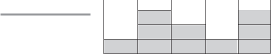
10.6 Implementing Dynamic Scoping 465
name at a given time, a very different approach can be taken. One variation of
shallow access is to have a separate stack for each variable name in a complete
program. Every time a new variable with a particular name is created by a dec-
laration at the beginning of a subprogram that has been called, the variable is
given a cell at the top of the stack for its name. Every reference to the name is
to the variable on top of the stack associated with that name, because the top
one is the most recently created. When a subprogram terminates, the lifetimes
of its local variables end, and the stacks for those variable names are popped.
This method allows fast references to variables, but maintaining the stacks at
the entrances and exits of subprograms is costly.
Figure 10.12 shows the variable stacks for the earlier example program in
the same situation as shown with the stack in Figure 10.11.
Another option for implementing shallow access is to use a central table
that has a location for each different variable name in a program. Along with
each entry, a bit called active is maintained that indicates whether the name
has a current binding or variable association. Any access to any variable can
then be to an offset into the central table. The offset is static, so the access
can be fast. SNOBOL implementations use the central table implementation
technique.
Maintenance of a central table is straightforward. A subprogram call
requires that all of its local variables be logically placed in the central table. If
the position of the new variable in the central table is already active—that is,
if it contains a variable whose lifetime has not yet ended (which is indicated
by the active bit)—that value must be saved somewhere during the lifetime of
the new variable. Whenever a variable begins its lifetime, the active bit in its
central table position must be set.
There have been several variations in the design of the central table and
in the way values are stored when they are temporarily replaced. One variation
is to have a “hidden” stack on which all saved objects are stored. Because sub-
program calls and returns, and thus the lifetimes of local variables, are nested,
this works well.
The second variation is perhaps the cleanest and least expensive to imple-
ment. A central table of single cells is used, storing only the current version
of each variable with a unique name. Replaced variables are stored in the
Figure 10.12
One method of using
shallow access to
implement dynamic
scoping
main main sub2 sub3 sub1
uvxzw
sub1 sub3 sub1
sub1 sub2
(The names in the stack cells indicate the
program units of the variable declaration.)

466 Chapter 10 Implementing Subprograms
activation record of the subprogram that created the replacement variable.
This is a stack mechanism, but it uses the stack that already exists, so the new
overhead is minimal.
The choice between shallow and deep access to nonlocal variables depends
on the relative frequencies of subprogram calls and nonlocal references. The
deep-access method provides fast subprogram linkage, but references to non-
locals, especially references to distant nonlocals (in terms of the call chain), are
costly. The shallow-access method provides much faster references to nonlocals,
especially distant nonlocals, but is more costly in terms of subprogram linkage.
SUMMARY
Subprogram linkage semantics requires many actions by the implementation.
In the case of “simple” subprograms, these actions are relatively simple. At the
call, the status of execution must be saved, parameters and the return address
must be passed to the called subprogram, and control must be transferred. At
the return, the values of pass-by-result and pass-by-value-result parameters
must be transferred back, as well as the return value if it is a function, execu-
tion status must be restored, and control transferred back to the caller. In
languages with stack-dynamic local variables and nested subprograms, subpro-
gram linkage is more complex. There may be more than one activation record
instance, those instances must be stored on the run-time stack, and static and
dynamic links must be maintained in the activation record instances. The static
link is to allow references to nonlocal variables in static-scoped languages.
Subprograms in languages with stack-dynamic local variables and nested
subprograms have two components: the actual code, which is static, and the
activation record, which is stack dynamic. Activation record instances contain
the formal parameters and local variables, among other things.
Access to nonlocal variables in a dynamic-scoped language can be imple-
mented by use of the dynamic chain or through some central variable table
method. Dynamic chains provide slow accesses but fast calls and returns. The
central table methods provide fast accesses but slow calls and returns.
REVIEW QUESTIONS
1. What is the definition used in this chapter for “simple” subprograms?
2. Which of the caller or callee saves execution status information?
3. What must be stored for the linkage to a subprogram?
4. What is the task of a linker?
5. What are the two reasons why implementing subprograms with stack-
dynamic local variables is more difficult than implementing simple
subprograms?

Problem Set 467
6. What is the difference between an activation record and an activation
record instance?
7. Why are the return address, dynamic link, and parameters placed in the
bottom of the activation record?
8. What kind of machines often use registers to pass parameters?
9. What are the two steps in locating a nonlocal variable in a static-scoped
language with stack-dynamic local variables and nested subprograms?
10. Define static chain, static_depth, nesting_depth, and chain_offset.
11. What is an EP, and what is its purpose?
12. How are references to variables represented in the static-chain method?
13. Name three widely used programming languages that do not allow
nested subprograms.
14. What are the two potential problems with the static-chain method?
15. Explain the two methods of implementing blocks.
16. Describe the deep-access method of implementing dynamic scoping.
17. Describe the shallow-access method of implementing dynamic scoping.
18. What are the two differences between the deep-access method for
nonlocal access in dynamic-scoped languages and the static-chain
method for static-scoped languages?
19. Compare the efficiency of the deep-access method to that of the shallow-
access method, in terms of both calls and nonlocal accesses.
PROBLEM SET
1. Show the stack with all activation record instances, including static and
dynamic chains, when execution reaches position 1 in the following skel-
etal program. Assume
Bigsub is at level 1.
procedure Bigsub is
procedure A is
procedure B is
begin -- of B
. . . 1
end; -- of B
procedure C is
begin -- of C
. . .
B;
. . .
end; -- of C

468 Chapter 10 Implementing Subprograms
begin -- of A
. . .
C;
. . .
end; -- of A
begin -- of Bigsub
. . .
A;
. . .
end; -- of Bigsub
2. Show the stack with all activation record instances, including static and
dynamic chains, when execution reaches position 1 in the following ske-
letal program. Assume Bigsub is at level 1.
procedure Bigsub is
MySum : Float;
procedure A is
X : Integer;
procedure B(Sum : Float) is
Y, Z : Float;
begin -- of B
. . .
C(Z)
. . .
end; -- of B
begin -- of A
. . .
B(X);
. . .
end; -- of A
procedure
C(Plums : Float) is
begin -- of C
. . . 1
end; -- of C
L : Float;
begin
-- of Bigsub
. . .
A;
. . .
end; -- of Bigsub
3. Show the stack with all activation record instances, including static and
dynamic chains, when execution reaches position 1 in the following skel-
etal program. Assume
Bigsub is at level 1.

Problem Set 469
procedure Bigsub is
procedure A(Flag : Boolean) is
procedure B is
. . .
A(false);
end; -- of B
begin -- of A
if flag
then B;
else C;
. . .
end; -- of A
procedure C is
procedure D is
. . . 1
end; -- of D
. . .
D;
end; -- of C
begin -- of Bigsub
. . .
A(true);
. . .
end; -- of Bigsub
The calling sequence for this program for execution to reach D is
Bigsub calls A
A
calls B
B
calls A
A
calls C
C
calls D
4. Show the stack with all activation record instances, including the
dynamic chain, when execution reaches position 1 in the following
ske letal program. This program uses the deep-access method to imple-
ment dynamic scoping.
void fun1() {
float a;
. . .
}
void fun2() {
int b, c;
. . .
}

470 Chapter 10 Implementing Subprograms
void fun3() {
float d;
. . . 1
}
void main() {
char e, f, g;
. . .
}
The calling sequence for this program for execution to reach fun3 is
main calls fun2
fun2
calls fun1
fun1
calls fun1
fun1
calls fun3
5. Assume that the program of Problem 4 is implemented using the
shallow-access method using a stack for each variable name. Show
the stacks for the time of the execution of fun3, assuming execution
found its way to that point through the sequence of calls shown in
Problem 4.
6. Although local variables in Java methods are dynamically allocated at the
beginning of each activation, under what circumstances could the value
of a local variable in a particular activation retain the value of the previ-
ous activation?
7. It is stated in this chapter that when nonlocal variables are accessed in a
dynamic-scoped language using the dynamic chain, variable names must
be stored in the activation records with the values. If this were actually
done, every nonlocal access would require a sequence of costly string
comparisons on names. Design an alternative to these string comparisons
that would be faster.
8. Pascal allows gotos with nonlocal targets. How could such statements
be handled if static chains were used for nonlocal variable access? Hint:
Consider the way the correct activation record instance of the static par-
ent of a newly enacted procedure is found (see Section 10.4.2).
9. The static-chain method could be expanded slightly by using two static
links in each activation record instance where the second points to the
static grandparent activation record instance. How would this approach
affect the time required for subprogram linkage and nonlocal references?
10. Design a skeletal program and a calling sequence that results in an acti-
vation record instance in which the static and dynamic links point to dif-
ferent activation-recorded instances in the run-time stack.

Programming Exercises 471
11. If a compiler uses the static chain approach to implementing blocks,
which of the entries in the activation records for subprograms are needed
in the activation records for blocks?
12. Examine the subprogram call instructions of three different architec-
tures, including at least one CISC machine and one RISC machine,
and write a short comparison of their capabilities. (The design of these
instructions usually determines at least part of the compiler writer’s
design of subprogram linkage.)
PROGRAMMING EXERCISES
1. Write a program that includes two subprograms, one that takes a single
parameter and performs some simple operation on that parameter and
one that takes 20 parameters and uses all of the parameters, but only for
one simple operation. The main program must call these two subpro-
grams a large number of times. Include in the program timing code to
output the run time of the calls to each of the two subprograms. Run
the program on a RISC machine and on a CISC machine and compare
the ratios of the time required by the two subprograms. Based on the
results, what can you say about the speed of parameter passing on the
two machines?
This page intentionally left blank


474 Chapter 11 Abstract Data Types and Encapsulation Constructs
I
n this chapter, we explore programming language constructs that support data
abstraction. Among the new ideas of the last 50 years in programming meth-
odologies and programming language design, data abstraction is one of the
most profound.
We begin by discussing the general concept of abstraction in programming and
programming languages. Data abstraction is then defined and illustrated with an
example. This topic is followed by descriptions of the support for data abstraction in
Ada, C++, Objective-C, Java, C#, and Ruby. To illuminate the similarities and differ-
ences in the design of the language facilities that support data abstraction, imple-
mentations of the same example data abstraction are given in Ada, C++, Objective-C,
Java, and Ruby. Next, the capabilities of Ada, C++, Java 5.0, and C# 2005 to build
parameterized abstract data types are discussed.
All the languages used in this chapter to illustrate the concepts and constructs
of abstract data types support object-oriented programming. The reason is that virtu-
ally all contemporary languages support object-oriented programming and nearly all
of those that do not, and yet support abstract data types, have faded into obscurity.
Constructs that support abstract data types are encapsulations of the data and
operations on objects of the type. Encapsulations that contain multiple types are
required for the construction of larger programs. These encapsulations and the asso-
ciated namespace issues are also discussed in this chapter.
Some programming languages support logical, as opposed to physical, encap-
sulations, which are actually used to encapsulate names. These are discussed in
Section 11.7.
11.1 The Concept of Abstraction
An abstraction is a view or representation of an entity that includes only the
most significant attributes. In a general sense, abstraction allows one to collect
instances of entities into groups in which their common attributes need not be
considered. For example, suppose we define birds to be creatures with the follow-
ing attributes: two wings, two legs, a tail, and feathers. Then, if we say a crow is a
bird, a description of a crow need not include those attributes. The same is true
for robins, sparrows, and yellow-bellied sapsuckers. These common attributes
in the descriptions of specific species of birds can be abstracted away, because all
species have them. Within a particular species, only the attributes that distinguish
that species need be considered. For example, crows have the attributes of being
black, being of a particular size, and being noisy. A description of a crow needs
to provide those attributes, but not the others that are common to all birds. This
results in significant simplification of the descriptions of members of the spe-
cies. A less abstract view of a species, that of a bird, may be considered when it
is necessary to see a higher level of detail, rather than just the special attributes.
In the world of programming languages, abstraction is a weapon against
the complexity of programming; its purpose is to simplify the programming
process. It is an effective weapon because it allows programmers to focus on
essential attributes, while ignoring subordinate attributes.

11.2 Introduction to Data Abstraction 475
The two fundamental kinds of abstraction in contemporary programming
languages are process abstraction and data abstraction.
The concept of process abstraction is among the oldest in programming
language design (Plankalkül supported process abstraction in the 1940s). All
subprograms are process abstractions because they provide a way for a program
to specify a process, without providing the details of how it performs its task
(at least in the calling program). For example, when a program needs to sort an
array of numeric data of some type, it usually uses a subprogram for the sorting
process. At the point where the sorting process is required, a statement such as
sortInt(list, listLen)
is placed in the program. This call is an abstraction of the actual sorting pro-
cess, whose algorithm is not specified. The call is independent of the algorithm
implemented in the called subprogram.
In the case of the subprogram sortInt, the only essential attributes are
the name of the array to be sorted, the type of its elements, the array’s length,
and the fact that the call to sortInt will result in the array being sorted.
The particular algorithm that sortInt implements is an attribute that is not
essential to the user. The user needs to see only the name and protocol of the
sorting subprogram to be able to use it.
The widespread use of data abstraction necessarily followed that of process
abstraction because an integral and essential part of every data abstraction is its
operations, which are defined as process abstractions.
11.2 Introduction to Data Abstraction
The evolution of data abstraction began in 1960 with the first version of
COBOL, which included the record data structure.
1
The C-based languages
have structs, which are also records. An abstract data type is a data structure, in
the form of a record, but which includes subprograms that manipulate its data.
Syntactically, an abstract data type is an enclosure that includes only the
data representation of one specific data type and the subprograms that provide
the operations for that type. Through access controls, unnecessary details of
the type can be hidden from units outside the enclosure that use the type.
Program units that use an abstract data type can declare variables of that type,
even though the actual representation is hidden from them. An instance of an
abstract data type is called an object.
One of the motivations for data abstraction is similar to that of process
abstraction. It is a weapon against complexity; a means of making large and/or
complicated programs more manageable. Other motivations for and advantages
of abstract data types are discussed later in this section.
1. Recall from Chapter 2, that a record is a data structure that stores fields, which have names
and can be of different types.
476 Chapter 11 Abstract Data Types and Encapsulation Constructs
Object-oriented programming, which is described in Chapter 12, is an
outgrowth of the use of data abstraction in software development, and data
abstraction is one of its fundamental components.
11.2.1 Floating-Point as an Abstract Data Type
The concept of an abstract data type, at least in terms of built-in types, is
not a recent development. All built-in data types, even those of Fortran I, are
abstract data types, although they are rarely called that. For example, consider
a floating-point data type. Most programming languages include at least one
of these. A floating-point type provides the means to create variables to store
floating-point data and also provides a set of arithmetic operations for manipu-
lating objects of the type.
Floating-point types in high-level languages employ a key concept in data
abstraction: information hiding. The actual format of the floating-point data
value in a memory cell is hidden from the user, and the only operations avail-
able are those provided by the language. The user is not allowed to create
new operations on data of the type, except those that can be constructed using
the built-in operations. The user cannot directly manipulate the parts of the
actual representation of values because that representation is hidden. It is this
feature that allows program portability between implementations of a particular
language, even though the implementations may use different representations
for particular data types. For example, before the IEEE 754 standard floating-
point representations appeared in the mid-1980s, there were several different
representations being used by different computer architectures. However, this
variation did not prevent programs that used floating-point types from being
portable among the various architectures.
11.2.2 User-Defined Abstract Data Types
A user-defined abstract data type should provide the same characteristics as
those of language-defined types, such as a floating-point type: (1) a type defi-
nition that allows program units to declare variables of the type but hides the
representation of objects of the type; and (2) a set of operations for manipulat-
ing objects of the type.
We now formally define an abstract data type in the context of user-defined
types. An abstract data type is a data type that satisfies the following conditions:
• The representation of objects of the type is hidden from the program units
that use the type, so the only direct operations possible on those objects are
those provided in the type’s definition.
• The declarations of the type and the protocols of the operations on objects
of the type, which provide the type’s interface, are contained in a single
syntactic unit. The type’s interface does not depend on the representation
of the objects or the implementation of the operations. Also, other program
units are allowed to create variables of the defined type.
11.2 Introduction to Data Abstraction 477
There are several benefits of information hiding. One of these is increased
reliability. Program units that use a specific abstract data type are called cli-
ents of that type. Clients cannot manipulate the underlying representations of
objects directly, either intentionally or by accident, thus increasing the integrity
of such objects. Objects can be changed only through the provided operations.
Another benefit of information hiding is it reduces the range of code and
number of variables of which a programmer must be aware when writing or
reading a part of the program. The value of a particular variable can only be
changed by code in a restricted range, making the code easier to understand
and less challenging to find sources of incorrect changes.
Information hiding also makes name conflicts less likely, because the scope
of variables is smaller.
Finally, consider the following advantage of information hiding: Suppose
that the original implementation of the stack abstraction uses a linked list rep-
resentation. At a later time, because of memory management problems with
that representation, the stack abstraction is changed to use a contiguous rep-
resentation (one that implements a stack in an array). Because data abstraction
was used, this change can be made in the code that defines the stack type, but
no changes will be required in any of the clients of the stack abstraction. In par-
ticular, the example code need not be changed. Of course, a change in protocol
of any of the operations would require changes in the clients.
Although the definition of abstract data types specifies that data members of
objects must be hidden from clients, many situations arise in which clients need to
access these data members. The common solution is to provide accessor methods,
sometimes called getters and setters, that allow clients indirect access to the so-
called hidden data—a better solution than simply making the data public, which
would provide direct access. There are three reasons why accessors are better:
1. Read-only access can be provided, by having a getter method but no
corresponding setter method.
2. Constraints can be included in setters. For example, if the data value
should be restricted to a particular range, the setter can enforce that.
3. The actual implementation of the data member can be changed without
affecting the clients if getters and setters are the only access.
Both specifying data in an abstract data type to be public and providing acces-
sor methods for that data are violations of the principles of abstract data types.
Some believe these are simply loopholes that make an imperfect design usable. As
we will see in Section 11.4.6.2, Ruby disallows making instance data public. How-
ever, Ruby also makes it very easy to create accessor functions. It is a challenge for
developers to design abstract data types in which all of the data is actually hidden.
The primary advantage of packaging the declarations of the type and its
operations in a single syntactic unit is that it provides a method of organizing
a program into logical units that can be compiled separately. In some cases,
the implementation is included with the type declaration; in other cases, it is
in a separate syntactic unit. The advantage of having the implementation of
the type and its operations in different syntactic units is that it increases the

478 Chapter 11 Abstract Data Types and Encapsulation Constructs
program’s modularity and it is a clear separation of design and implementa-
tion. If both the declarations and the definitions of types and operations are
in the same syntactic unit, there must be some means of hiding from client
program units the parts of the unit that specify the definitions.
11.2.3 An Example
A stack is a widely applicable data structure that stores some number of data
elements and only allows access to the data element at one of its ends, the top.
Suppose an abstract data type is to be constructed for a stack that has the fol-
lowing abstract operations:
Note that some implementations of abstract data types do not require the
create and destroy operations. For example, simply defining a variable to be of
an abstract data type may implicitly create the underlying data structure and
initialize it. The storage for such a variable may be implicitly deallocated at the
end of the variable’s scope.
A client of the stack type could have a code sequence such as the following:
. . .
create(stk1);
push(stk1, color1);
push(stk1, color2);
temp = top(stk1);
. . .
11.3 Design Issues for Abstract Data Types
A facility for defining abstract data types in a language must provide a syntactic
unit that encloses the declaration of the type and the prototypes of the subpro-
grams that implement the operations on objects of the type. It must be possible
to make these visible to clients of the abstraction. This allows clients to declare
variables of the abstract type and manipulate their values. Although the type
create(stack) Creates and possibly initializes a stack object
destroy(stack) Deallocates the storage for the stack
empty(stack) A predicate (or Boolean) function that returns
true if the specified stack is empty and false
otherwise
push(stack, element) Pushes the specified element on the specified
stack
pop(stack) Removes the top element from the specified
stack
top(stack) Returns a copy of the top element from the
specified stack

11.4 Language Examples 479
name must have external visibility, the type representation must be hidden. The
type representation and the definitions of the subprograms that implement the
operations may appear inside or outside this syntactic unit.
Few, if any, general built-in operations should be provided for objects of
abstract data types, other than those provided with the type definition. There
simply are not many operations that apply to a broad range of abstract data types.
Among these are assignment and comparisons for equality and inequality. If the
language does not allow users to overload assignment, the assignment operation
must be included in the abstraction. Comparisons for equality and inequality should
be predefined in the abstraction in some cases but not in others. For example, if
the type is implemented as a pointer, equality may mean pointer equality, but the
designer may want it to mean equality of the structures referenced by the pointers.
Some operations are required by many abstract data types, but because they
are not universal, they often must be provided by the designer of the type. Among
these are iterators, accessors, constructors, and destructors. Iterators were discussed
in Chapter 8. Accessors provide a form of access to data that is hidden from direct
access by clients. Constructors are used to initialize parts of newly created objects.
Destructors are often used to reclaim heap storage that may be used by parts of
abstract data type objects in languages that do not do implicit storage reclamation.
As stated earlier, the enclosure for an abstract data type defines a single
data type and its operations. Many contemporary languages, including C++,
Objective-C, Java, and C#, directly support abstract data types. One alterna-
tive approach is to provide a more generalized encapsulation construct that can
define any number of entities, any of which can be selectively specified to be
visible outside the enclosing unit. Ada uses this approach. These enclosures are
not abstract data types but rather are generalizations of abstract data types. As
such, they can be used to define abstract data types. Although we discuss Ada’s
encapsulation construct in this section, we treat it as a minimal encapsulation
for single data types. Generalized encapsulations are the topic of Section 11.6.
So, the first design issue for abstract data types is the form of the container
for the interface to the type. The second design issue is whether abstract data
types can be parameterized. For example, if the language supports parameter-
ized abstract data types, one could design an abstract data type for some struc-
ture that could store elements of any type. Parameterized abstract data types
are discussed in Section 11.5. The third design issue is what access controls are
provided and how such controls are specified. Finally, the language designer
must decide whether the specification of the type is physically separate from its
implementation (or whether that is a developer choice).
11.4 Language Examples
The concept of data abstraction had its origins in SIMULA 67, although that
language did not provide complete support for abstract data types, because
it did not include a way to hide implementation details. In this section, we
describe the support for data abstraction provided by Ada, C++, Objective-C,
Java, C#, and Ruby.

interview
C++: Its Birth, Its Ubiquitousness,
and Common Criticisms
BJARNE STROUSTRUP
Bjarne Stroustrup is the designer and original implementer of C++ and the author
of
The C++ Programming Language
and
The Design and Evolution of C++.
His
research interests include distributed systems, simulation, design, programming, and
programming languages. Dr. Stroustrup is the College of Engineering Professor in
Computer Science at Texas A&M University. He is actively involved in the ANSI/ISO
standardization of C++. After more than two decades at AT&T, he retains a link with
AT&T Labs, doing research as a member of the Information and Software Systems
Research Lab. He is an ACM Fellow, an AT&T Bell Laboratories Fellow, and an
AT&T Fellow. In 1993, Stroustrup received the ACM Grace Murray Hopper Award
“for his early work laying the foundations for the C++ programming language. Based
on the foundations and Dr. Stroustrup’s continuing efforts, C++ has become one of
the most influential programming languages in the history of computing.”
A BRIEF HISTORY OF YOU AND COMPUTING
What were you working on, and where, before you
joined Bell Labs in the early 1980s?
At Bell Labs,
I was doing research in the general area of distributed
systems. I joined in 1979. Before that, I was finishing
my Ph.D. in that field in Cambridge University.
Did you immediately start on “C with Classes”
(which would later become C++)?
I worked on a
few projects related to distributed computing before
starting on C with Classes and during the development
of that and of C++. For example, I was trying to find a
way to distribute the UNIX kernel across several com-
puters and helped a lot of projects build simulators.
Was it an interest in mathematics that got you
into this profession?
I signed up for a degree in
“mathematics with computer science” and my mas-
ter’s degree is officially a math degree. I—wrongly—
thought that computing was some kind of applied
math. I did a couple of years of math and rate myself a
poor mathematician, but that’s still much better than
not knowing math. At the time I signed up, I had never
even seen a computer. What I love about computing is
the programming rather than the more mathematical
fields.
DISSECTING A SUCCESSFUL LANGUAGE
I’d like to work backward, listing some items I
think make C++ ubiquitous, and get your reac-
tion. It’s “open source,” nonproprietary, and
standardized by ANSI/ISO.
The ISO C++ standard
is important. There are many independently developed
and evolving C++ implementations. Without a standard
for them to adhere to and a standards process to help
coordinate the evolution of C++, a chaos of dialects
would erupt.
It is also important that there are both open-source
and commercial implementations available. In addi-
tion, for many users, it is crucial that the standard
provides a measure of protection from manipulation by
implementation providers.
The ISO standards process is open and democratic.
The C++ committee rarely meets with fewer than 50
people present and typically more than eight nations
are represented at each meeting. It is not just a ven-
dors’ forum.
It’s ideal for systems programming (which, at the
time C++ was born, was the largest sector of the mar-
ket developing code).
Yes, C++ is a strong contender for any systems-
programming project. It is also effective for embedded
480

systems programming, which is currently the fastest-
growing sector. Yet another growth area for C++
is high-performance numeric/engineering/scientific
programming.
Its object-oriented nature and inclusion of
classes/libraries make programming more effi-
cient and transparent.
C++ is a multiparadigm
programming language. That is, it supports several
fundamental styles of programming (including object-
oriented programming) and combinations of those
styles. When used well, this leads to cleaner, more flex-
ible, and more efficient libraries than can be provided
using just one paradigm. The C++ standard library
containers and algorithms, which is basically a generic
programming framework, is an example. When used
together with (object-oriented) class hierarchies, the
result is an unsurpassed combination of type safety,
efficiency, and flexibility.
Its incubation in the AT&T development environ-
ment.
AT&T Bell Labs provided an environment that
was crucial for C++’s development. The labs were
an exceptionally rich source of challenging problems
and a uniquely supportive environment for practical
research. C++ emerged from the same research lab as
C did and benefited from the same intellectual tradi-
tion, experience, and exceptional people. Throughout,
AT&T supported the standardization of C++. However,
C++ was not the beneficiary of a massive marketing
campaign, like many modern languages. That’s simply
not the way the labs work.
Did I miss anything on your top list? Undoubtedly.
Now, let me paraphrase from the C++ critiques
and get your reactions: It’s huge/unwieldy. The
“hello world” problem is 10 times larger in C++
than in C.
C++ is certainly not a small language,
but then few modern languages are. If a language is
small, you tend to need huge libraries to get work done
and often have to rely on conventions and extensions.
I prefer to have key parts of the inevitable complex-
ity in the language where it can be seen, taught, and
effectively standardized rather than hidden elsewhere
in a system. For most purposes, I don’t consider C++
unwieldy. The C++ “hello world” program isn’t larger
than its C equivalent on my machine, and it shouldn’t
be on yours.
In fact, the object code for the C++ version of the
“hello world” program is smaller than the C version
on my machine. There is no language reason why the
one version should be larger than the other. It is all an
issue of how the implementor organized the libraries.
If one version is significantly larger than the other,
report the problem to the implementor of the larger
version.
It’s tougher to program in C++ (compared with C).
(Something the critics say.) Even you once admit-
ted it, saying something about shooting your-
self in the foot with C versus C++.
Yes, I did say
something along the lines of “C makes it easy to shoot
yourself in the foot; C++ makes it harder, but when you
do, C++ blows your whole leg off.” What people tend
to miss is that what I said about C++ is to a varying
extent true for all powerful languages. As you protect
people from simple dangers, they get themselves into
new and less obvious problems. Someone who avoids
the simple problems may simply be heading for a not-
so-simple one. One problem with very supporting and
protective environments is that the hard problems may
be discovered too late or be too hard to remedy once
discovered. Also, a rare problem is harder to find than
a frequent one because you don’t suspect it.
It’s appropriate for embedded systems of today
but not for the Internet software of today. C++ is
suitable for embedded systems today.
It is also
suitable—and widely used—for “Internet software”
today. For example, have a look at my “C++ applica-
tions” Web page. You’ll notice that some of the major
Web service providers, such as Amazon, Adobe, Google,
Quicken, and Microsoft, critically rely on C++. Gaming
is a related area in which you find heavy C++ use.
Did I miss another one that you get a lot? Sure.
481
482 Chapter 11 Abstract Data Types and Encapsulation Constructs
11.4.1 Abstract Data Types in Ada
Ada provides an encapsulation construct that can be used to define a single
abstract data type, including the ability to hide its representation. Ada 83 was
one of the first languages to offer full support for abstract data types.
11.4.1.1 Encapsulation
The encapsulating constructs in Ada are called packages. A package can have
two parts, each of which is also is called a package. These are called the package
specification, which provides the interface of the encapsulation (and perhaps
more), and the body package, which provides the implementation of most, if
not all, of the entities named in the associated package specification. Not all
packages have a body part (packages that encapsulate only types and constants
do not have or need bodies).
A package specification and its associated body package share the same
name. The reserved word
body in a package header identifies it as being a
body package. A package specification and its body package may be compiled
separately, provided the package specification is compiled first. Client code can
also be compiled before the body package is compiled or even written, for that
matter. This means that once the package specification is written, work can
begin on both the client code and the body package.
11.4.1.2 Information Hiding
The designer of an Ada package that defines a data type can choose to make
the type entirely visible to clients or provide only the interface information.
Of course, if the representation is not hidden, then the defined type is not an
abstract data type. There are two approaches to hiding the representation from
clients in the package specification. One is to include two sections in the pack-
age specification—one in which entities are visible to clients and one that hides
its contents. For an abstract data type, a declaration appears in the visible part
of the specification, providing only the name of the type and the fact that its
representation is hidden. The representation of the type appears in a part of the
specification called the private part, which is introduced by the reserved word
private. The private clause is always at the end of the package specification.
The private clause is visible to the compiler but not to client program units.
The second way to hide the representation is to define the abstract data
type as a pointer and provide the pointed-to structure’s definition in the body
package, whose entire contents are hidden from clients.
Types that are declared to be private are called private types. Private data
types have built-in operations for assignment and comparisons for equality and
inequality. Any other operation must be declared in the package specification
that defined the type.
The reason that a type’s representation appears in the package specification
at all has to do with compilation issues. Client code can see only the package
11.4 Language Examples 483
specification (not the body package), but the compiler must be able to allocate
objects of the exported type when compiling the client. Furthermore, the client
is compilable when only the package specification for the abstract data type has
been compiled and is present. Therefore, the compiler must be able to deter-
mine the size of an object from the package specification. So, the representation
of the type must be visible to the compiler but not to the client code. This is
exactly the situation specified by the private clause in a package specification.
An alternative to private types is a more restricted form: limited private
types. Nonpointer limited private types are described in the private section
of a package specification, as are nonpointer private types. The only syntactic
difference is that limited private types are declared to be limited private
in the visible part of the package specification. The semantic difference is that
objects of a type that is declared limited private have no built-in operations.
Such a type is useful when the usual predefined operations of assignment and
comparison are not meaningful or useful. For example, assignment and com-
parison are rarely used for stacks.
11.4.1.3 An Example
The following is the package specification for a stack abstract data type:
package Stack_Pack is
-- The visible entities, or public interface
type Stack_Type is limited private;
Max_Size : constant := 100;
function Empty(Stk : in Stack_Type) return Boolean;
procedure Push(Stk : in out Stack_Type;
Element : in Integer);
procedure Pop(Stk : in out Stack_Type);
function Top(Stk : in Stack_Type) return Integer;
-- The part that is hidden from clients
private
type List_Type is array (1..Max_Size) of Integer;
type Stack_Type is
record
List : List_Type;
Topsub : Integer range 0..Max_Size := 0;
end record;
end Stack_Pack;
Notice that no create or destroy operations are included, because they are not
necessary.
The body package for Stack_Pack is as follows:
with Ada.Text_IO; use Ada.Text_IO;
package body Stack_Pack is
484 Chapter 11 Abstract Data Types and Encapsulation Constructs
function Empty(Stk: in Stack_Type) return Boolean is
begin
return Stk.Topsub = 0;
end Empty;
procedure Push(Stk : in out Stack_Type;
Element : in Integer) is
begin
if Stk.Topsub >= Max_Size then
Put_Line("ERROR - Stack overflow");
else
Stk.Topsub := Stk.Topsub + 1;
Stk.List(Topsub) := Element;
end if;
end Push;
procedure Pop(Stk : in out Stack_Type) is
begin
if Empty(Stk)
then Put_Line("ERROR - Stack underflow");
else Stk.Topsub := Stk.Topsub - 1;
end if;
end Pop;
function Top(Stk : in Stack_Type) return Integer is
begin
if Empty(Stk)
then Put_Line("ERROR - Stack is empty");
else return Stk.List(Stk.Topsub);
end if;
end Top;
end Stack_Pack;
The first line of the code of this body package contains two clauses: a with
and a use. The with clause makes the names defined in external packages
visible; in this case Ada.Text_IO, which provides functions for input and
output of text. The use clause eliminates the need for explicit qualification
of the references to entities from the named package. The issues of access
to external encapsulations and name qualifications are further discussed in
Section 11.7.
The body package must have subprogram definitions with headings that
match the subprogram headings in the associated package specification. The
package specification promises that these subprograms will be defined in the
associated body package.
The following procedure,
Use_Stacks, is a client of package Stack_Pack.
It illustrates how the package might be used.

11.4 Language Examples 485
with Stack_Pack;
use Stack_Pack;
procedure Use_Stacks is
Topone : Integer;
Stack : Stack_Type; -- Creates a Stack_Type object
begin
Push(Stack, 42);
Push(Stack, 17);
Topone := Top(Stack);
Pop(Stack);
. . .
end Use_Stacks;
A stack is a silly example for most contemporary languages, because sup-
port for stacks is included in their standard class libraries. However, stacks
provide a simple example we can use to allow comparisons of the languages
discussed in this section.
11.4.1.4 Evaluation
Ada, along with Modula-2, was the first commercial language to support
abstract data types.
2
Although Ada’s design of abstract data types may seem
complicated and repetitious, it clearly provides what is necessary.
11.4.2 Abstract Data Types in C++
C++, which was first released in 1985, was created by adding features to C. The
first important additions were those to support object-oriented programming.
Because one of the primary components of object-oriented programming is
abstract data types, C++ obviously is required to support them.
While Ada provides an encapsulation that can be used to simulate abstract
data types, C++ provides two constructs that are very similar to each other, the
class and the struct, which more directly support abstract data types. Because
structs are most commonly used when only data is included, we do not discuss
them further here.
C++ classes are types; as stated previously, Ada packages are more gen-
eralized encapsulations that can define any number of types. A program unit
that gains visibility to an Ada package can access any of its public entities
directly by their names. A C++ program unit that declares an instance of a
class can also access any of the public entities in that class, but only through
an instance of the class. This is a cleaner and more direct way to provide
abstract data types.
2. The language CLU, which was an academic research language, rather than a commercial
language, was the first to support abstract data types.

486 Chapter 11 Abstract Data Types and Encapsulation Constructs
11.4.2.1 Encapsulation
The data defined in a C++ class are called data members; the functions
(methods) defined in a class are called member functions. Data members and
member functions appear in two categories: class and instance. Class members
are associated with the class; instance members are associated with the instances
of the class. In this chapter, only the instance members of a class are discussed.
All of the instances of a class share a single set of member functions, but each
instance has its own set of the class’s data members. Class instances can be
static, stack dynamic, or heap dynamic. If static or stack dynamic, they are
referenced directly with value variables. If heap dynamic, they are referenced
through pointers. Stack dynamic instances of classes are always created by the
elaboration of an object declaration. Furthermore, the lifetime of such a class
instance ends when the end of the scope of its declaration is reached. Heap
dynamic class instances are created with the
new operator and destroyed with
the delete operator. Both stack- and heap-dynamic classes can have pointer
data members that reference heap dynamic data, so that even though a class
instance is stack dynamic, it can include data members that reference heap
dynamic data.
A member function of a class can be defined in two distinct ways: The
complete definition can appear in the class, or only in its header. When both
the header and the body of a member function appear in the class definition,
the member function is implicitly inlined. Recall that this means that its code
is placed in the caller’s code, rather than requiring the usual call and return
linkage process. If only the header of a member function appears in the class
definition, its complete definition appears outside the class and is separately
compiled. The rationale for allowing member functions to be inlined was
to save function call overhead in real-time applications, in which run-time
efficiency is of utmost importance. The downside of inlining member func-
tions is that it clutters the class definition interface, resulting in a reduction
in readability.
Placing member function definitions outside the class definition
separates specification from implementation, a common goal of modern
programming.
11.4.2.2 Information Hiding
A C++ class can contain both hidden and visible entities (meaning they are
either hidden from or visible to clients of the class). Entities that are to be hid-
den are placed in a private clause, and visible, or public, entities appear in a
public clause. The public clause therefore describes the interface to class
instances.
3
3. There is also a third category of visibility, protected, which is discussed in the context of
inheritance in Chapter 12.
11.4 Language Examples 487
11.4.2.3 Constructors and Destructors
C++ allows the user to include constructor functions in class definitions, which
are used to initialize the data members of newly created objects. A constructor
may also allocate the heap-dynamic data that are referenced by the pointer
members of the new object. Constructors are implicitly called when an object
of the class type is created. A constructor has the same name as the class whose
objects it initializes. Constructors can be overloaded, but of course each con-
structor of a class must have a unique parameter profile.
A C++ class can also include a function called a destructor, which is
implicitly called when the lifetime of an instance of the class ends. As stated
earlier, stack-dynamic class instances can contain pointer members that refer-
ence heap-dynamic data. The destructor function for such an instance can
include a
delete operator on the pointer members to deallocate the heap
space they reference. Destructors are often used as a debugging aid, in which
case they simply display or print the values of some or all of the object’s data
members before those members are deallocated. The name of a destructor is
the class’s name, preceded by a tilde (~).
Neither constructors nor destructors have return types, and neither use
return statements. Both constructors and destructors can be explicitly called.
11.4.2.4 An Example
Our examle of a C++ abstract data type is, once again, a stack:
#include <iostream.h>
class Stack {
private: //** These members are visible only to other
//** members and friends (see Section 11.6.4)
int *stackPtr;
int maxLen;
int topSub;
public: //** These members are visible to clients
Stack() { //** A constructor
stackPtr = new int [100];
maxLen = 99;
topSub = -1;
}
~Stack() {delete [] stackPtr;}; //** A destructor
void push(int number) {
if (topSub == maxLen)
cerr << "Error in push--stack is full\n";
else stackPtr[++topSub] = number;
}
void pop() {
if (empty())
488 Chapter 11 Abstract Data Types and Encapsulation Constructs
cerr << "Error in pop--stack is empty\n";
else topSub--;
}
int top() {
if (empty())
cerr << "Error in top--stack is empty\n";
else
return (stackPtr[topSub]);
}
int empty() {return (topSub == -1);}
}
We discuss only a few aspects of this class definition, because it is not neces-
sary to understand all of the details of the code. Objects of the Stack class are
stack dynamic but include a pointer that references heap-dynamic data. The
Stack class has three data members—stackPtr, maxLen, and topSub—all
of which are private. stackPtr is used to reference the heap-dynamic data,
which is the array that implements the stack. The class also has four public
member functions—
push, pop, top, and empty—as well as a constructor and
a destructor. All of the member function definitions are included in this class,
although they could have been externally defined. Because the bodies of the
member functions are included, they are all implicitly inlined. The constructor
uses the new operator to allocate an array of 100 int elements from the heap.
It also initializes maxLen and topSub.
The following is an example program that uses the Stack abstract data
type:
void main() {
int topOne;
Stack stk; //** Create an instance of the Stack class
stk.push(42);
stk.push(17);
topOne = stk.top();
stk.pop();
. . .
}
Following is a definition of the Stack class with only prototypes of the
member functions. This code is stored in a header file with the .h file name
extension. The definitions of the member functions follow the class definition.
These use the scope resolution operator, ::, to indicate the class to which
they belong. These definitions are stored in a code file with the file name
extension .cpp.
// Stack.h - the header file for the Stack class
#include <iostream.h>
11.4 Language Examples 489
class Stack {
private: //** These members are visible only to other
//** members and friends (see Section 11.6.4)
int *stackPtr;
int maxLen;
int topSub;
public: //** These members are visible to clients
Stack(); //** A constructor
~Stack(); //** A destructor
void push(int);
void pop();
int top();
int empty();
}
// Stack.cpp - the implementation file for the Stack class
#include <iostream.h>
#include "Stack.h"
using std::cout;
Stack::Stack() { //** A constructor
stackPtr = new int [100];
maxLen = 99;
topSub = -1;
}
Stack::~Stack() {delete [] stackPtr;}; //** A destructor
void Stack::push(int number) {
if (topSub == maxLen)
cerr << "Error in push--stack is full\n";
else stackPtr[++topSub] = number;
}
void Stack::pop() {
if (topSub == -1)
cerr << "Error in pop--stack is empty\n";
else topSub--;
}
int top() {
if (topSub == -1)
cerr << "Error in top--stack is empty\n";
else
return (stackPtr[topSub]);
}
int Stack::empty() {return (topSub == -1);}
490 Chapter 11 Abstract Data Types and Encapsulation Constructs
11.4.2.5 Evaluation
C++ support for abstract data types, through its class construct, is similar in
expressive power to that of Ada, through its packages. Both provide effective
mechanisms for encapsulation and information hiding of abstract data types.
The primary difference is that classes are types, whereas Ada packages are
more general encapsulations. Furthermore, the package construct of Ada was
designed for more than data abstraction, as discussed in Chapter 12.
11.4.3 Abstract Data Types in Objective-C
As has been previously stated, Objective-C is similar to C++ in that its initial
design was the C language with extensions to support object-oriented program-
ming. One of the fundamental differences between the two is that Objective-C
uses the syntax of Smalltalk for its method calls.
11.4.3.1 Encapsulation
The interface part of an Objective-C class is defined in a container called an
interface with the following general syntax:
@interface class-name: parent-class {
instance variable declarations
}
method prototypes
@end
The first and last lines, which begin with at signs (@), are directives.
The implementation of a class is packaged in a container naturally named
implementation, which has the following syntax:
@implementation class-name
method definitions
@end
As in C++, in Objective-C classes are types.
Method prototypes have the following syntax:
(+ | -)(return-type) method-name [: (formal-parameters)];
When present, the plus sign indicates that the method is a class method; a
minus sign indicates an instance method. The brackets around the formal
parameters indicate that they are optional. Neither the parentheses nor the
colon are present when there are no parameters. As in most other languages
that support object-oriented programming, all instances of an Objective-C
class share a single copy of its instance methods, but each instance has its own
copy of the instance data.
11.4 Language Examples 491
The syntactic form of the formal parameter list is different from that of
the more common languages, C, C++, Java, and C#. If there is one parameter,
its type is specified in parentheses before the parameter’s name, as in the fol-
lowing method prototype:
-(void) meth1: (int) x;
This method’s name is meth1: (note the colon). A method with two parameters
could appear as in the following example method prototype:
-(int) meth2: (int) x second: (float) y;
In this case, the method’s name is meth2:second:, although that is obviously
a poorly chosen name. The last part of the name (
second) could have been
omitted, as in the following:
-(int) meth2: (int) x: (float) y;
In this case, the name of the method is meth2::.
Method definitions are like method prototypes except that they have a
brace-delimited sequence of statements in place of the semicolon.
The syntax of a call to a method with no parameters is as follows:
[object-name method-name];
If a method takes one parameter, a colon is attached to the method name
and the parameter follows. There is no other punctuation between the method
name and the parameter. For example, a call to a method named add1 on the
object referenced by myAdder that takes one parameter, in this case the lit-
eral 7, would appear as follows:
[myAdder add1: 7];
If a method takes two parameters and has only one part to its name, a colon
follows the first parameter and the second parameter follows that. No other
punctuation is used between the two parameters. If there are more parameters,
this pattern is repeated. For example, if
add1 takes three parameters and has
no other parts to its name, it could be called with the following:
[myAdder add1: 7: 5: 3];
A method could have multiple parameters and multiple parts to its name,
as in the previous example:
-(int) meth2: (int) x second: (float) y;
An example call to this method follows:
[myObject meth2: 7 second: 3.2];
492 Chapter 11 Abstract Data Types and Encapsulation Constructs
Constructors in Objective-C are called initializers; they only provide ini-
tial values. They can be given any name, and as a result they must be explicitly
called. Constructors return a reference to the new object, so their type is always
a pointer to the class-name. They use a return statement that returns self, a
reference to the current object.
An object is created in Objective-C by calling alloc. Typically, after call-
ing alloc, the constructor of the class is explicitly called. These two calls can
be and usually are cascaded, as in the following statement, which creates an
object of Adder class with alloc and then calls its constructor, init, on the
new object, and puts the address of the new object in myAdder:
Adder *myAdder = [[Adder alloc]init];
All class instances are heap dynamic and are referenced through reference
variables.
C programs nearly always import a header file for input and output
functions,
stdio.h. In Objective-C, a header file is usually imported that
has the prototypes of a variety of often required functions, including those
for input and output, as well as some needed data. This is done with the
following:
#import <Foundation/Foundation.h>
Importing the Foundation.h header file creates some data for the pro-
gram. So, the first thing the main function should do is allocate and initialize
a pool of storage for this data. This is done with the following statement:
NSAutoreleasePool * pool = [[NSAutoreleasePool alloc] init];
Just before the return statement in main, this pool is released with a call to the
drain method of the pool object, as in the following statement:
[pool drain];
11.4.3.2 Information Hiding
Objective-C uses the directives, @private and @public, to specify the
access levels of the instance variables in a class definition. These are used as
the reserved words public and private are used in C++. The difference is
that the default in Objective-C is protected, whereas it is private in C++. Unlike
most programming languages that support object-oriented programming, in
Objective-C there is no way to restrict access to a method.
In Objective-C, the convention is that the name of a getter method for
an instance variable is the variable’s name. The name of the setter method is
the word
set with the capitalized variable’s name attached. So, for a variable
named sum, the getter method would be named sum and the setter method
11.4 Language Examples 493
would be named setSum. Assuming that sum is an int variable, these methods
could be defined as follows:
// The getter for sum
-(int) sum {
return sum;
}
// The setter for sum
-(void) setSum: (int) s {
sum = s;
}
If the getter and setter method for a particular variable does not impose
any constraints on their actions, they can be automatically generated by the
Objective-C compiler. This is done by listing the instance variables for which
getters and setters are to be generated on the property directive in the interface
section, as in the following:
@property int sum;
In the implementation section, the variables are listed in a synthesize direc-
tive, as in the following:
@synthesize sum;
Variables for which getters and setters are generated by the com-
piler are often called properties and the accessor methods are said to be
synthesized.
The getters and setters of instance variables can be used in two ways, either
in method calls or in dot notation, as if they were publically accessible. For
example, if we have defined a getter and a setter for the variable sum, they could
be used as in the following:
[myObject setSum: 100];
newSum = [myObject sum];
or as if they were publically accessible, as in the following:
myObject.sum = 100;
newSum = myObject.sum;
11.4.3.3 An Example
Following are the definitions of the interface and implementation of the stack
class in Objective-C:
494 Chapter 11 Abstract Data Types and Encapsulation Constructs
// stack.m - interface and implementation of a simple stack
#import <Foundation/Foundation.h>
// Interface section
@interface Stack: NSObject {
int stackArray [100];
int stackPtr;
int maxLen;
int topSub;
}
-(void) push: (int) number;
-(void) pop;
-(int) top;
-(int) empty;
@end
// Implementation section
@implementation Stack
-(Stack *) initWith {
maxLen = 100;
topSub = -1;
stackPtr = stackArray;
return self;
}
-(void) push: (int) number {
if (topSub == maxLen)
NSLog(@"Error in push--stack is full");
else
stackPtr[++topSub] = number;
}
-(void) pop {
if (topSub == -1)
NSLog(@"Error in pop--stack is empty");
else
topSub--;
}
-(int) top {
if (topSub >= 0)
return stackPtr[topSub]);
else
NSLog(@"Error in top--stack is empty");
11.4 Language Examples 495
}
-(int) empty {
return topSub == -1);
}
int main (int argc, char *argv[]) {
int temp;
NSAutoreleasePool *pool = [[NSAutoreleasePool alloc]
init];
Stack *myStack = [[Stack alloc]initWith];
[myStack push: 5];
[myStack push: 3];
temp = [myStack top];
NSLog(@"Top element is:%i", temp);
[myStack pop];
temp = [myStack top];
NSLog(@"Top element is:%i", temp);
temp = [myStack top];
[myStack pop];
[myStack release];
[pool drain];
return 0;
}
@end
The output of this program is as follows:
Top element is: 3
Top element is: 5
Error in top--stack is empty
Error in pop--stack is empty
Screen output from an Objective-C program is created with a call to a
method with the odd-looking name, NSLog, which takes a literal string as its
parameter. Literal strings are created with an at sign (@) followed by a quoted
string. If an output string includes the values of variables, the names of the
variables are included as parameters in the call to NSLog. The positions in the
literal string for the values are marked with format codes, for example %i for
an integer and %f for a floating-point value in scientific notation, as is similar
to C’s printf function.
11.4.3.4 Evaluation
The support in Objective-C for abstract data types is adequate. Some find
it odd that it uses syntactic forms from two very different languages, Small-
talk (for its method calls) and C (for nearly everything else). Also, its use of

496 Chapter 11 Abstract Data Types and Encapsulation Constructs
directives in place of language constructs to indicate class interfaces and imple-
mentation sections also differs from most other programming languages. One
minor deficiency is the lack of a way to restrict access to methods. So, even
methods meant only to be used inside a class are accessible to clients. Another
minor deficiency is that constructors must be explicitly called, thereby requir-
ing programmers to remember to call them, and also leading to further clutter
in the client program.
11.4.4 Abstract Data Types in Java
Java support for abstract data types is similar to that of C++. There are, how-
ever, a few important differences. All objects are allocated from the heap and
accessed through reference variables. Methods in Java must be defined com-
pletely in a class. A method body must appear with its corresponding method
header.
4
Therefore, a Java abstract data type is both declared and defined in a
single syntactic unit. A Java compiler can inline any method that is not over-
ridden. Definitions are hidden from clients by declaring them to be private.
Rather than having private and public clauses in its class definitions, in
Java access modifiers can be attached to method and variable definitions. If an
instance variable or method does not have an access modifier, it has package
access, which is discussed in Section 11.7.2.
11.4.4.1 An Example
The following is a Java class definition for our stack example:
class StackClass {
private int [] stackRef;
private int maxLen,
topIndex;
public StackClass() { // A constructor
stackRef = new int [100];
maxLen = 99;
topIndex = -1;
}
public void push(int number) {
if (topIndex == maxLen)
System.out.println("Error in push—stack is full");
else stackRef[++topIndex] = number;
}
public void pop() {
if (empty())
System.out.println("Error in pop—stack is empty");
4. Java interfaces are an exception to this—an interface has method headers but cannot include
their bodies.

11.4 Language Examples 497
else --topIndex;
}
public int top() {
if (empty()) {
System.out.println("Error in top—stack is empty");
return 9999;
}
else
return (stackRef[topIndex]);
}
public boolean empty() {return (topIndex == -1);}
}
An example class that uses StackClass follows:
public class TstStack {
public static void main(String[] args) {
StackClass myStack = new StackClass();
myStack.push(42);
myStack.push(29);
System.out.println("29 is: " + myStack.top());
myStack.pop();
System.out.println("42 is: " + myStack.top());
myStack.pop();
myStack.pop(); // Produces an error message
}
}
One obvious difference is the lack of a destructor in the Java version, obviated
by Java’s implicit garbage collection.
5
11.4.4.2 Evaluation
Although different in some primarily cosmetic ways, Java’s support for abstract
data types is similar to that of C++. Java clearly provides for what is necessary
to design abstract data types.
11.4.5 Abstract Data Types in C#
Recall that C# is based on both C++ and Java and that it also includes some new
constructs. Like Java, all C# class instances are heap dynamic. Default construc-
tors, which provide initial values for instance data, are predefined for all classes.
These constructors provide typical initial values, such as 0 for int types and
false for boolean types. A user can furnish one or more constructors for any
5. In Java, the finalize method serves as a kind of destructor.
498 Chapter 11 Abstract Data Types and Encapsulation Constructs
class he or she defines. Such constructors can assign initial values to some or all
of the instance data of the class. Any instance variable that is not initialized in a
user-defined constructor is assigned a value by the default constructor.
Although C# allows destructors to be defined, because it uses garbage col-
lection for most of its heap objects, destructors are rarely used.
11.4.5.1 Encapsulation
As mentioned in Section 11.4.2, C++ includes both classes and structs, which
are nearly identical constructs. The only difference is that the default access
modifier for class is private, whereas for structs it is public. C# also has
structs, but they are very different from those of C++. In C#, structs are, in a
sense, lightweight classes. They can have constructors, properties, methods,
and data fields and can implement interfaces but do not support inheritance.
One other important difference between structs and classes in C# is that structs
are value types, as opposed to reference types. They are allocated on the run-
time stack, rather than the heap. If they are passed as parameters, like other
value types, by default they are passed by value. All C# value types, including
all of its primitive types, are actually structs. Structs can be created by declaring
them, like other predefined value types, such as
int or float. They can also
be created with the new operator, which calls a constructor to initialize them.
Structs are used in C# primarily to implement relatively small simple types
that need never be base types for inheritance. They are also used when it is
convenient for the objects of the type to be stack as opposed to heap allocated.
11.4.5.2 Information Hiding
C# uses the private and protected access modifiers exactly as they are
used in Java.
C# provides properties, which it inherited from Delphi, as a way of imple-
menting getters and setters without requiring explicit method calls by the cli-
ent. As with Objective-C, properties provide implicit access to specific private
instance data. For example, consider the following simple class and client code:
public class Weather {
public int DegreeDays { //** DegreeDays is a property
get {
return degreeDays;
}
set {
if(value < 0 || value > 30)
Console.WriteLine(
"Value is out of range: {0}", value);
else
degreeDays = value;
}
11.4 Language Examples 499
}
private int degreeDays;
. . .
}
. . .
Weather w = new Weather();
int degreeDaysToday, oldDegreeDays;
. . .
w.DegreeDays = degreeDaysToday;
. . .
oldDegreeDays = w.DegreeDays;
In the class Weather, the property DegreeDays is defined. This property pro-
vides a getter method and a setter method for access to the private data member,
degreeDays. In the client code following the class definition, degreeDays is
treated as if it were a public-member variable, although access to it is available
through the property only. Notice the use of the implicit variable value in the
setter method. This is the mechanism by which the new value of the property
is referenced.
The stack example is not shown here in C#. The only difference between
the Java version in Section 11.4.4.1 and the C# version is the output method
calls and the use of
bool instead of boolean for the return type of the empty
method.
11.4.6 Abstract Data Types in Ruby
Ruby provides support for abstract data types through its classes. In terms of
capabilities, Ruby classes are similar to those in C++ and Java.
11.4.6.1 Encapsulation
In Ruby, a class is defined in a compound statement opened with the class
reserved word and closed with
end. The names of instance variables have
a special syntactic formthey must begin with at signs (@). Instance meth-
ods have the same syntax as functions in Ruby: They begin with the def
reserved word and end with end. Class methods are distinguished from
instance methods by having the class name appended to the beginning of
their names with a period separator. For example, in a class named Stack,
a class method’s name would begin with Stack. Constructors in Ruby are
named initialize. Because the constructor cannot be overloaded, there
only can be one per class.
Classes in Ruby are dynamic in the sense that members can be added at
any time. This is done by simply including additional class definitions that
specify the new members. Moreover, even predefined classes of the language,
such as
String, can be extended. For example, consider the following class
definition:
500 Chapter 11 Abstract Data Types and Encapsulation Constructs
class myClass
def meth1
. . .
end
end
This class could be extended by adding a second method, meth2, with a second
class definition:
class myClass
def meth2
. . .
end
end
Methods can also be removed from a class. This is done by providing
another class definition in which the method to be removed is sent to the
method
remove_method as a parameter. The dynamic classes of Ruby are
another example of a language designer trading readability (and as a conse-
quence, reliability) for flexibility. Allowing dynamic changes to classes clearly
adds flexibility to the language, while harming readability. To determine the
behavior of a class at a particular point in a program, one must find all of its
definitions in the program and consider all of them.
11.4.6.2 Information Hiding
Access control for methods in Ruby is dynamic, so access violations are detected
only during execution. The default method access is public, but it can also be
protected or private. There are two ways to specify the access control, both of
which use functions with the same names as the access levels, private and
public. One way is to call the appropriate function without parameters. This
resets the default access for subsequently defined methods in the class. For
example,
class MyClass
def meth1
. . .
end
. . .
private
def meth7
. . .
end
. . .
end # of class MyClass
11.4 Language Examples 501
The alternative is to call the access control functions with the names of
the specific methods as parameters. For example, the following is semantically
equivalent to the previous class definition:
class MyClass
def meth1
. . .
end
. . .
def meth7
. . .
end
private :meth7, . . .
end # of class MyClass
In Ruby, all data members of a class are private, and that cannot be changed.
So, data members can be accessed only by the methods of the class, some of
which may be accessor methods. In Ruby, instance data that are accessible
through accessor methods are called attributes.
For an instance variable named @sum, the getter and setter methods would
be as follows:
def sum
@sum
end
def sum=(new_sum)
@sum = new_sum
end
Notice that getters are given the name of the instance variable minus the @. The
names of setter methods are the same as those of the corresponding getters,
except they have an equal sign (=) attached.
Getters and setters can be implicitly generated by the Ruby system by
including calls to attr_reader and attr_writer, respectively, in the class
definition. The parameters to these are the symbols of the attribute’s names,
as is illustrated in the following:
attr_reader :sum, :total
attr_writer :sum
11.4.6.3 An Example
Following is the stack example written in Ruby:
# Stack.rb - defines and tests a stack of maximum length
# 100, implemented in an array
502 Chapter 11 Abstract Data Types and Encapsulation Constructs
class StackClass
# Constructor
def initialize
@stackRef = Array.new(100)
@maxLen = 100
@topIndex = -1
end
# push method
def push(number)
if @topIndex == @maxLen
puts "Error in push - stack is full"
else
@topIndex = @topIndex + 1
@stackRef[@topIndex] = number
end
end
# pop method
def pop
if empty
puts "Error in pop - stack is empty"
else
@topIndex = @topIndex - 1
end
end
# top method
def top
if empty
puts "Error in top - stack is empty"
else
@stackRef[@topIndex]
end
end
# empty method
def empty
@topIndex == -1
end
end # of Stack class
# Test code for StackClass
myStack = StackClass.new
myStack.push(42)

11.5 Parameterized Abstract Data Types 503
myStack.push(29)
puts "Top element is (should be 29): #{myStack.top}"
myStack.pop
puts "Top element is (should be 42): #{myStack.top}"
myStack.pop
# The following pop should produce an
# error message - stack is empty
myStack.pop
Recall that the notation #{variable} converts the value of the variable to a
string, which is then inserted into the string in which it appears. This class
defines a stack structure that can store objects of any type.
11.4.6.4 Evaluation
Recall that in Ruby, everything is an object and arrays are actually arrays of
references to objects. That clearly makes this stack more flexible than the
similar examples in Ada, C++, and Java. Furthermore, simply by passing the
desired maximum length to the constructor, objects of this class could have
any given maximum length. Of course, because arrays in Ruby have dynamic
length, the class could be modified to implement stack objects that are not
restricted to any length, except that imposed by the machine’s memory capac-
ity. Because the names of class and instance variables have different forms,
Ruby has a slight readability advantage over the other languages discussed
in this section.
11.5 Parameterized Abstract Data Types
It is often convenient to be able to parameterize abstract data types. For exam-
ple, we should be able to design a stack abstract data type that can store any
scalar type elements rather than be required to write a separate stack abstrac-
tion for every different scalar type. Note that this is only an issue for static
typed languages. In a dynamic typed language like Ruby, any stack implicitly
can store any type elements. In fact, different elements of the stack could be
of different types. In the following four subsections, the capabilities of Ada,
C++, Java 5.0, and C# 2005 to construct parameterized abstract data types are
discussed.
11.5.1 Ada
Generic procedures in Ada were discussed and illustrated in Chapter 9. Pack-
ages can also be generic, so we can construct generic, or parameterized, abstract
data types.
504 Chapter 11 Abstract Data Types and Encapsulation Constructs
The Ada stack abstract data type example shown in Section 11.4.1 suffers
two restrictions: (1) Stacks of its type can store only integer type elements, and
(2) the stacks can have only up to 100 elements. Both of these restrictions can
be eliminated by using a generic package, which can be instantiated for other
element types and any desirable size. (This is a generic instantiation, which is
very different from the instantiation of a class to create an object.) The follow-
ing package specification describes the interface of a generic stack abstract data
type with these features:
generic
Max_Size : Positive; -- A generic parameter for stack
-- size
type Element_Type is private; -- A generic parameter
-- for element type
package Generic_Stack is
-- The visible entities, or public interface
type Stack_Type is limited private;
function Empty(Stk : in Stack_Type) return Boolean;
procedure Push(Stk : in out Stack_Type;
Element : in Element_Type);
procedure Pop(Stk : in out Stack_Type);
function Top(Stk : in Stack_Type) return Element_Type;
-- The hidden part
private
type List_Type is array (1..Max_Size) of Element_Type;
type Stack_Type is
record
List : List_Type;
Topsub : Integer range 0..Max_Size := 0;
end record;
end Generic_Stack;
The body package for Generic_Stack is the same as the body package for
Stack_Pack in the Section 11.4.1.3 except that the type of the Element for-
mal parameter in Push and Top is Element_Type instead of Integer.
The following statement instantiates Generic_Stack for a stack of 100
Integer type elements:
package Integer_Stack is new Generic_Stack(100, Integer);
One could also build an abstract data type for a stack of length 500 for Float
elements, as in
package Float_Stack is new Generic_Stack(500, Float);
These instantiations build two different source code versions of the
Generic_Stack package at compile time.
11.5 Parameterized Abstract Data Types 505
11.5.2 C++
C++ also supports parameterized abstract data types. To make the example C++
stack class of Section 11.4.2.4 generic in the stack size, only the constructor
function needs to be changed, as in the following:
Stack(int size) {
stackPtr = new int [size];
maxLen = size - 1;
topSub = -1;
}
The declaration for a stack object now may appear as follows:
Stack stk(150);
The class definition for Stack can include both constructors, so users can
use the default-size stack or specify some other size.
The element type of the stack can be made generic by making the class
a templated class. Then, the element type can be a template parameter. The
definition of the templated class for a stack type is as follows:
#include <iostream.h>
template <typename Type> // Type is the template parameter
class Stack {
private:
Type *stackPtr;
int maxLen;
int topSub;
public:
// A constructor for 100 element stacks
Stack() {
stackPtr = new Type [100];
maxLen = 99;
topSub = -1;
}
// A constructor for a given number of elements
Stack(int size) {
stackPtr = new Type [size];
maxLen = size - 1;
topSub = -1;
}
~Stack() {delete stackPtr;}; // A destructor
void push(Type number) {
if (topSub == maxLen)
cout << "Error in push—stack is full\n";
else stackPtr[++ topSub] = number;
506 Chapter 11 Abstract Data Types and Encapsulation Constructs
}
void pop() {
if (empty())
cout << "Error in pop—stack is empty\n";
else topSub --;
}
Type top() {
if (empty())
cerr << "Error in top--stack is empty\n";
else
return (stackPtr[topSub]);
}
int empty() {return (topSub == -1);}
}
As in Ada, C++ templated classes are instantiated to become typed classes
at compile time. For example, an instance of the templated Stack class, as well
as an instance of the typed class, can be created with the following declaration:
Stack<int> myIntStack;
However, if an instance of the templated Stack class has already been
created for the int type, the typed class need not be created.
11.5.3 Java 5.0
Java 5.0 supports a form of parameterized abstract data types in which the generic
parameters must be classes. Recall that these were briefly discussed in Chapter 9.
The most common generic types are collection types, such as LinkedList
and ArrayList, which were in the Java class library before support for gener-
ics was added. The original collection types stored Object class instances, so
they could store any objects (but not primitive types). Therefore, the collection
types have always been able to store multiple types (as long as they are classes).
There were three issues with this: First, every time an object was removed from
the collection, it had to be cast to the appropriate type. Second, there was no
error checking when elements were added to the collection. This meant that
once the collection was created, objects of any class could be added to the col-
lection, even if the collection was meant to store only Integer objects. Third,
the collection types could not store primitive types. So, to store int values in
an ArrayList, the value first had to be put in an Integer class instance. For
example, consider the following code:
//* Create an ArrayList object
ArrayList myArray = new ArrayList();
//* Create an element
myArray.add(0, new Integer(47));
11.5 Parameterized Abstract Data Types 507
//* Get first object
Integer myInt = (Integer)myArray.get(0);
In Java 5.0, the collection classes, the most commonly used of which is
ArrayList, became a generic class. Such classes are instantiated by calling
new on the class constructor and passing it the generic parameter in pointed
brackets. For example, the ArrayList class can be instantiated to store
Integer objects with the following statement:
ArrayList <Integer> myArray = new ArrayList <Integer>();
This new class overcomes two of the problems with pre-Java 5.0 collections.
Only Integer objects can be put into the myArray collection. Furthermore,
there is no need to cast an object being removed from the collection.
Java 5.0 also includes interfaces for collections for lists, queues, and sets.
Users also can define generic classes in Java 5.0. For example, we could
have the following:
public class MyClass<T> {
. . .
}
This class could be instantiated with the following:
MyClass<String> myString;
There are some drawbacks to these user-defined generic classes. For
one thing, they cannot store primitives. Second, the elements cannot be
indexed. Elements must be added to user-defined generic collections with
the add method. Next, we implement the generic stack example using an
Array List. Note that the last element of an ArrayList is found using
the
size method, which returns the number of elements in the structure.
Elements are deleted from the structure with the remove method. Follow-
ing is the generic class:
import java.util.*;
public class Stack2<T> {
private ArrayList<T> stackRef;
private int maxLen;
public Stack2() { // A constructor
stackRef = new ArrayList<T> ();
maxLen = 99;
}
public void push(T newValue) {
if (stackRef.size() == maxLen)
508 Chapter 11 Abstract Data Types and Encapsulation Constructs
System.out.println("Error in push—stack is full");
else
stackRef.add(newValue);
}
public void pop() {
if (empty())
System.out.println("Error in pop—stack is empty");
else
stackRef.remove(stackRef.size() - 1);
}
public T top() {
if (empty()) {
System.out.println("Error in top—stack is empty");
return null;
}
else
return (stackRef.get(stackRef.size() - 1));
}
public boolean empty() {return (stackRef.isEmpty());}
This class could be instantiated for the String type with the following:
Stack2<String> myStack = new Stack2<String>();
Recall from Chapter 9, that Java 5.0 supports wildcard classes. For exam-
ple, Collection<?> is a wildcard class for all collection classes. This allows
a method to be written that can accept any collection type as a parameter.
Because a collection can itself be generic, the Collection<?> class is in a
sense a generic of a generic class.
Some care must be taken with objects of the wildcard type. For example,
because the components of a particular object of this type have a type, other
type objects cannot be added to the collection. For example, consider
Collection<?> c = new ArrayList<String>();
It would be illegal to use the add method to put something into this collection
unless its type were String.
A generic class can easily be defined in Java 5.0 that will work only for a
restricted set of types. For example, a class can declare a variable of the generic
type and call a method such as compareTo through that variable. If the class
is instantiated for a type that does not include a compareTo method, the
class cannot be used. To prevent a generic class from being instantiated for a
type that does not support compareTo, it could be defined with the following
generic parameter:
<T extends Comparable>

11.6 Encapsulation Constructs 509
Comparable is the interface in which compareTo is declared. If this generic
type is used on a class definition, the class cannot be instantiated for any type
that does not implement Comparable. The choice of the reserved word
extends seems odd here, but its use is related to the concept of a subtype.
Apparently, the designers of Java did not want to add another more connotative
reserved word to the language.
11.5.4 C# 2005
As was the case with Java, the first version of C# defined collection classes that
stored objects of any class. These were
ArrayList, Stack, and Queue. These
classes had the same problems as the collection classes of pre-Java 5.0.
Generic classes were added to C# in its 2005 version. The five predefined
generic collections are
Array, List, Stack, Queue, and Dictionary (the
Dictionary class implements hashes). Exactly as in Java 5.0, these classes
eliminate the problems of allowing mixed types in collections and requiring
casts when objects are removed from the collections.
As with Java 5.0, users can define generic classes in C# 2005. One capability
of the user-defined C# generic collections is that any of them can be defined to
allow its elements to be indexed (accessed through subscripting). Although the
indexes are usually integers, an alternative is to use strings as indexes.
One capability that Java 5.0 provides that C# 2005 does not is wildcard
classes.
11.6 Encapsulation Constructs
The first five sections of this chapter discuss abstract data types, which are
minimal encapsulations.
6
This section describes the multiple-type encapsula-
tions that are needed for larger programs.
11.6.1 Introduction
When the size of a program reaches beyond a few thousand lines, two practi-
cal problems become evident. From the programmer’s point of view, having
such a program appear as a single collection of subprograms or abstract data
type definitions does not impose an adequate level of organization on the pro-
gram to keep it intellectually manageable. The second practical problem for
larger programs is recompilation. For relatively small programs, recompiling
the whole program after each modification is not costly. But for large programs,
the cost of recompilation is significant. So, there is an obvious need to find
ways to avoid recompilation of the parts of a program that are not affected by
6. In the case of Ada, the package encapsulation can be used for single types and also for mul-
tiple types.
510 Chapter 11 Abstract Data Types and Encapsulation Constructs
a change. The obvious solution to both of these problems is to organize pro-
grams into collections of logically related code and data, each of which can be
compiled without recompilation of the rest of the program. An encapsulation
is such a collection.
Encapsulations are often placed in libraries and made available for reuse in
programs other than those for which they were written. People have been writ-
ing programs with more than a few thousand lines for at least the last 50 years,
so techniques for providing encapsulations have been evolving for some time.
In languages that allow nested subprograms, programs can be organized
by nesting subprogram definitions inside the logically larger subprograms that
use them. This can be done in Ada, Fortran 95, Python, and Ruby. As discussed
in Chapter 5, however, this method of organizing programs, which uses static
scoping, is far from ideal. Therefore, even in languages that allow nested sub-
programs, they are not used as a primary organizing encapsulation construct.
11.6.2 Encapsulation in C
C does not provide complete support for abstract data types, although both
abstract data types and multiple-type encapsulations can be simulated.
In C, a collection of related functions and data definitions can be placed in
a file, which can be independently compiled. Such a file, which acts as a library,
has an implementation of its entities. The interface to such a file, including
data, type, and function declarations, is placed in a separate file called a header
file. Type representations can be hidden by declaring them in the header file
as pointers to struct types. The complete definitions of such struct types need
only appear in the implementation file. This approach has the same draw-
backs as the use of pointers as abstract data types in Ada packages—namely,
the inherent problems of pointers and the potential confusion with assignment
and comparisons of pointers.
The header file, in source form, and the compiled version of the imple-
mentation file are furnished to clients. When such a library is used, the header
file is included in the client code, using an
#include preprocessor specifica-
tion, so that references to functions and data in the client code can be type
checked. The
#include specification also documents the fact that the client
program depends on the library implementation file. This approach effectively
separates the specification and implementation of an encapsulation.
Although these encapsulations work, they create some insecurities. For
example, a user could simply cut and paste the definitions from the header
file into the client program, rather than using
#include. This would work,
because #include simply copies the contents of its operand file into the file
in which the #include appears. However, there are two problems with this
approach. First, the documentation of the dependence of the client program on
the library (and its header file) is lost. Second, the author of the library could
change the header file and the implementation file, but the client could attempt
to use the new implementation file (not realizing it had changed) but with the
old header file, which the user had copied into his or her client program. For
11.6 Encapsulation Constructs 511
example, a variable x could have been defined to be int type in the old header
file, which the client code still uses, although the implementation code has
been recompiled with the new header file, which defines x to be float. So,
the implementation code was compiled with x as an int but the client code was
compiled with x as a float. The linker does not detect this error.
Thus, it is the user’s responsibility to ensure that both the header and
implementation files are up-to-date. This is often done with a make utility.
11.6.3 Encapsulation in C++
C++ provides two different kinds of encapsulation—header and implementa-
tion files can be defined as in C, or class headers and definitions can be defined.
Because of the complex interplay of C++ templates and separate compilation,
the header files of C++ template libraries often include complete definitions of
resources, rather than just data declarations and subprogram protocols; this is
due in part to the use of the C linker for C++ programs.
When nontemplated classes are used for encapsulations, the class header
file has only the prototypes of the member functions, with the function defini-
tions provided outside the class in a code file, as in the last example in Section
11.4.2.4. This clearly separates interface from implementation.
One language design problem that results from having classes but no gen-
eralized encapsulation construct is that sometimes when operations are defined
that use two different classes of objects, the operation does not naturally belong
in either class. For example, suppose we have an abstract data type for matrices
and one for vectors and need a multiplication operation between a vector and
a matrix. The multiplication code must have access to the data members of
both the vector and the matrix classes, but neither of those classes is the natural
home for the code. Furthermore, regardless of which is chosen, access to the
members of the other is a problem. In C++, these kinds of situations can be
handled by allowing nonmember functions to be “friends” of a class. Friend
functions have access to the private entities of the class where they are declared
to be friends. For the matrix/vector multiplication operation, one C++ solu-
tion is to define the operation outside both the matrix and the vector classes
but define it to be a friend of both. The following skeletal code illustrates this
scenario:
class Matrix; //** A class declaration
class Vector {
friend Vector multiply(const Matrix&, const Vector&);
. . .
};
class Matrix { //** The class definition
friend Vector multiply(const Matrix&, const Vector&);
. . .
};
//** The function that uses both Matrix and Vector objects

512 Chapter 11 Abstract Data Types and Encapsulation Constructs
Vector multiply(const Matrix& m1, const Vector& v1) {
. . .
}
In addition to functions, whole classes can be defined to be friends of a
class; then all the private members of the class are visible to all of the members
of the friend class.
11.6.4 Ada Packages
Ada package specifications can include any number of data and subprogram
declarations in their public and private sections. Therefore, they can include
interfaces for any number of abstract data types, as well as any other program
resources. So, the package is a multiple-type encapsulation construct.
Consider the situation described in Section 11.6.3 of the vector and matrix
types and the need for methods with access to the private parts of both, which
is handled in C++ with friend functions. In Ada, both the matrix and the vector
types could be defined in a single Ada package, which obviates the need for
friend functions.
11.6.5 C# Assemblies
C# includes a larger encapsulation construct than a class. The construct is the
one used by all of the .NET programming languages: the assembly. Assemblies
are built by .NET compilers. A .NET application consists of one or more
assemblies. An assembly is a file
7
that appears to application programs to be a
single dynamic link library (.dll)
8
or an executable (.exe). An assembly
defines a module, which can be separately developed. An assembly includes
several different components. One of the primary components of an assembly
is its programming code, which is in an intermediate language, having been
compiled from its source language. In .NET, the intermediate language is
named Common Intermediate Language (CIL). It is used by all .NET lan-
guages. Because its code is in CIL, an assembly can be used on any architecture,
device, or operating system. When executed, the CIL is just-in-time compiled
to native code for the architecture on which it is resident.
In addition to the CIL code, a .NET assembly includes metadata that describes
every class it defines, as well as all external classes it uses. An assembly also includes
a list of all assemblies referenced in the assembly and an assembly version number.
7. An assembly can consist of any number of files.
8. A dynamic link library (DLL) is a collection of classes and methods that are individu-
ally linked to an executing program when needed during execution. Therefore, although a
program has access to all of the resources in a particular DLL, only the parts that are actu-
ally used are ever loaded and linked to the program. DLLs have been part of the Windows
programming environment since Windows first appeared. However, the DLLs of .NET are
quite different from those of previous Windows systems.

11.7 Naming Encapsulations 513
In the .NET world, the assembly is the basic unit of deployment of soft-
ware. Assemblies can be private, in which case they are available to just one
application, or public, which means any application can use them.
As mentioned previously, C# has an access modifier, internal. An
internal member of a class is visible to all classes in the assembly in which
it appears.
Java has a file structure that is similar to an assembly called a Java Archive
( JAR). It is also used for deployment of Java software systems. JARs are built
with the Java utility jar, rather than a compiler.
11.7 Naming Encapsulations
We have considered encapsulations to be syntactic containers for logically
related software resources—in particular, abstract data types. The purpose of
these encapsulations is to provide a way to organize programs into logical units
for compilation. This allows parts of programs to be recompiled after isolated
changes. There is another kind of encapsulation that is necessary for construct-
ing large programs: a naming encapsulation.
A large program is usually written by many developers, working somewhat
independently, perhaps even in different geographic locations. This requires
the logical units of the program to be independent, while still able to work
together. It also creates a naming problem: How can independently working
developers create names for their variables, methods, and classes without acci-
dentally using names already in use by some other programmer developing a
different part of the same software system?
Libraries are the origin of the same kind of naming problems. Over the past
two decades, large software systems have become progressively more dependent
on libraries of supporting software. Nearly all software written in contemporary
programming languages requires the use of large and complex standard librar-
ies, in addition to application-specific libraries. This widespread use of multiple
libraries has necessitated new mechanisms for managing names. For example,
when a developer adds new names to an existing library or creates a new library,
he or she must not use a new name that conflicts with a name already defined in
a client’s application program or in some other library. Without some language
processor assistance, this is virtually impossible, because there is no way for the
library author to know what names a client’s program uses or what names are
defined by the other libraries the client program might use.
Naming encapsulations define name scopes that assist in avoiding these
name conflicts. Each library can create its own naming encapsulation to prevent
its names from conflicting with the names defined in other libraries or in client
code. Each logical part of a software system can create a naming encapsulation
with the same purpose.
Naming encapsulations are logical encapsulations, in the sense that they
need not be contiguous. Several different collections of code can be placed in
the same namespace, even though they are stored in different places. In the
514 Chapter 11 Abstract Data Types and Encapsulation Constructs
following sections, we briefly describe the uses of naming encapsulations in
C++, Java, Ada, and Ruby.
11.7.1 C++ Namespaces
C++ includes a specification, namespace, that helps programs manage the
problem of global namespaces. One can place each library in its own namespace
and qualify the names in the program with the name of the namespace when
the names are used outside that namespace. For example, suppose there is an
abstract data type header file that implements stacks. If there is concern that
some other library file may define a name that is used in the stack abstract data
type, the file that defines the stack could be placed in its own namespace. This
is done by placing all of the declarations for the stack in a namespace block, as
in the following:
namespace myStackSpace {
// Stack declarations
}
The implementation file for the stack abstract data type could reference
the names declared in the header file with the scope resolution operator,
::, as in
myStackSpace::topSub
The implementation file could also appear in a namespace block specifica-
tion identical to the one used on the header file, which would make all of the
names declared in the header file directly visible. This is definitely simpler, but
slightly less readable, because it is less obvious where a specific name in the
implementation file is declared.
Client code can gain access to the names in the namespace of the header
file of a library in three different ways. One way is to qualify the names from
the library with the name of the namespace. For example, a reference to the
variable topSub could appear as follows:
myStackSpace::topSub
This is exactly the way the implementation code could reference it if the imple-
mentation file was not in the same namespace.
The other two approaches use the using directive. This directive can be
used to qualify individual names from a namespace, as with
using myStackSpace::topSub;
which makes topSub visible, but not any other names from the myStackSpace
namespace.

11.7 Naming Encapsulations 515
The using directive can also be used to qualify all of the names from a
namespace, as in the following:
using namespace myStackSpace;
Code that includes this directive can directly access the names defined in the
namespace, as in
p = topSub;
Be aware that namespaces are a complicated feature of C++, and we have
introduced only the simplest part of the story here.
C# includes namespaces that are much like those of C++.
11.7.2 Java Packages
Java includes a naming encapsulation construct: the package. Packages can
contain more than one type
9
definition, and the types in a package are partial
friends of one another. Partial here means that the entities defined in a type in
a package that either are public or protected (see Chapter 12) or have no access
specifier are visible to all other types in the package.
Entities without access modifiers are said to have package scope, because they
are visible throughout the package. Java therefore has less need for explicit friend
declarations and does not include the friend functions or friend classes of C++.
The resources defined in a file are specified to be in a particular package
with a package declaration, as in
package stkpkg;
The package declaration must appear as the first line of the file. The
resources of every file that does not include a package declaration are implicitly
placed in the same unnamed package.
The clients of a package can reference the types defined in the package using
fully qualified names. For example, if the package
stkpkg has a class named
myStack, that class can be referenced in a client of stkpkg as stkpkg.myStack.
Likewise, a variable in the myStack object named topSub could be referenced
as stkpkg.myStack.topSub. Because this approach can quickly become cum-
bersome when packages are nested, Java provides the import declaration, which
allows shorter references to type names defined in a package. For example, sup-
pose the client includes the following:
import stkpkg.myStack;
Now, the class myStack can be referenced by just its name. To be able to access
all of the type names in the package, an asterisk can be used on the import
9. By type here we mean either a class or an interface.
516 Chapter 11 Abstract Data Types and Encapsulation Constructs
statement in place of the type name. For example, if we wanted to import all
of the types in stkpkg, we could use the following:
import stkpkg.*;
Note that Java’s import is only an abbreviation mechanism. No otherwise
hidden external resources are made available with import. In fact, in Java
nothing is implicitly hidden if it can be found by the compiler or class loader
(using the package name and the CLASSPATH environment variable).
Java’s import documents the dependencies of the package in which it
appears on the packages named in the import. These dependencies are less
obvious when import is not used.
11.7.3 Ada Packages
Ada packages, which often are used to encapsulate libraries, are defined in hier-
archies, which correspond to the directory hierarchies in which they are stored.
For example, if subPack is a package defined as a child of the package pack, the
subPack code file would appear in a subdirectory of the directory that stored
the pack package. The standard class libraries of Java are also defined in a
hierarchy of packages and are stored in a corresponding hierarchy of directories.
As discussed in Section 11.4.1, packages also define namespaces. Vis-
ibility to a package from a program unit is gained with the with clause. For
example, the following clause makes the resources and namespace of the
package Ada.Text_IO available.
with Ada.Text_IO;
Access to the names defined in the namespace of Ada.Text_IO must be quali-
fied. For example, the Put procedure from Ada.Text_IO must be accessed as
Ada.Text_IO.Put
To access the names in Ada.Text_IO without qualification, the use clause
can be used, as in
use Ada.Text_IO;
With this clause, the Put procedure from Ada.Text_IO can be accessed sim-
ply as Put. Ada’s use is similar to Java’s import.
11.7.4 Ruby Modules
Ruby classes serve as namespace encapsulations, as do the classes of other lan-
guages that support object-oriented programming. Ruby has an additional
naming encapsulation, called a module. Modules typically define collections of

Summary 517
methods and constants. So, modules are convenient for encapsulating libraries
of related methods and constants, whose names are in a separate namespace so
there are no name conflicts with other names in a program that uses the mod-
ule. Modules are unlike classes in that they cannot be instantiated or subclassed
and do not define variables. Methods that are defined in a module include the
module’s name in their names. For example, consider the following skeletal
module definition:
module MyStuff
PI = 3.14159265
def MyStuff.mymethod1(p1)
. . .
end
def MyStuff.mymethod2(p2)
. . .
end
end
Assuming the MyStuff module is stored in its own file, a program that wants
to use the constant and methods of
MyStuff must first gain access to the
module. This is done with the
require method, which takes the file name in
the form of a string literal as a parameter. Then, the constants and methods of
the module can be accessed through the module’s name. Consider the follow-
ing code that uses our example module,
MyStuff, which is stored in the file
named myStuffMod:
require 'myStuffMod'
. . .
MyStuff.mymethod1(x)
. . .
Modules are further discussed in Chapter 12.
SUMMARY
The concept of abstract data types, and their use in program design, was a
milestone in the development of programming as an engineering discipline.
Although the concept is relatively simple, its use did not become convenient
and safe until languages were designed to support it.
The two primary features of abstract data types are the packaging of data
objects with their associated operations and information hiding. A language
may support abstract data types directly or simulate them with more general
encapsulations.
Ada provides encapsulations called packages that can be used to simulate
abstract data types. Packages normally have two parts: a specification, which
518 Chapter 11 Abstract Data Types and Encapsulation Constructs
presents the client interface, and a body, which supplies the implementation
of the abstract data type. Data type representations can appear in the package
specification but be hidden from clients by putting them in the private clause of
the package. The abstract type itself is defined to be private in the public part of
the package specification. Private types have built-in operations for assignment
and comparison for equality and inequality.
C++ data abstraction is provided by classes. Classes are types, and
instances can be either stack or heap dynamic. A member function (method)
can have its complete definition appear in the class or have only the proto-
col given in the class and the definition placed in another file, which can be
separately compiled. C++ classes can have two clauses, each prefixed with
an access modifier: private or public. Both constructors and destructors can
be given in class definitions. Heap-allocated objects must be explicitly deal-
located with
delete.
As with C++, Objective-C data abstractions are classes. Classes are types
and all are heap dynamic. Methods declarations must appear in interface sec-
tions of classes and method definitions must appear in implementation sections.
Constructors are called initializers; they must be explicitly called. Instance
variables can be private or public. Access to methods cannot be restricted.
Method calls use syntax that is similar to that used by Smalltalk. Objective-C
supports properties and access methods for properties can be furnished by the
compiler.
Java data abstractions are similar to those of C++, except all Java objects
are allocated from the heap and are accessed through reference variables.
Also, all objects are garbage collected. Rather than having access modifiers
attached to clauses, in Java the modifiers appear on individual declarations
(or definitions).
C# supports abstract data types with both classes and structs. Its structs are
value types and do not support inheritance. C# classes are similar to those of Java.
Ruby supports abstract data types with its classes. Ruby’s classes differ
from those of most other languages in that they are dynamic—members can
be added, deleted, or changed during execution.
Ada, C++, Java 5.0, and C# 2005 allow their abstract data types to be
parameterized—Ada through its generic packages, C++ through its templated
classes, and Java 5.0 and C# through their collection classes and interfaces and
user-defined generic classes.
To support the construction of large programs, some contemporary lan-
guages include multiple-type encapsulation constructs, which can contain a
collection of logically related types. An encapsulation may also provide access
control to its entities. Encapsulations provide the programmer with a method
of organizing programs that also facilitates recompilation.
C++, C#, Java, Ada, and Ruby provide naming encapsulations. For Ada
and Java, they are named packages; for C++ and C#, they are namespaces; for
Ruby, they are modules. Partially because of the availability of packages, Java
does not have friend functions or friend classes. In Ada, packages can be used
as naming encapsulations.

Review Questions 519
REVIEW QUESTIONS
1. What are the two kinds of abstractions in programming languages?
2. Define abstract data type.
3. What are the advantages of the two parts of the definition of abstract data
type?
4. What are the language design requirements for a language that supports
abstract data types?
5. What are the language design issues for abstract data types?
6. Explain how information hiding is provided in an Ada package.
7. To what is the private part of an Ada package specification visible?
8. What is the difference between
private and limited private types
in Ada?
9. What is in an Ada package specification? What about a body package?
10. What is the use of the Ada with clause?
11. What is the use of the Ada use clause?
12. What is the fundamental difference between a C++ class and an Ada
package?
13. From where are C++ objects allocated?
14. In what different places can the definition of a C++ member function
appear?
15. What is the purpose of a C++ constructor?
16. What are the legal return types of a constructor?
17. Where are all Java methods defined?
18. How are C++ class instances created?
19. How are the interface and implementation sections of an Objective-C
class specified?
20. Are Objective-C classes types?
21. What is the access level of Objective-C methods?
22. What is the origin of the syntax of method calls in Objective-C?
23. When are constructors implicitly called in Objective-C?
24. Why are properties better than specifying an instance variable to be
public?
25. From where are Java class instances allocated?
26. Why does Java not have destructors?
27. Where are all Java methods defined?
28. Where are Java classes allocated?
29. Why are destructors not as frequently needed in Java as they are in C++?

520 Chapter 11 Abstract Data Types and Encapsulation Constructs
30. What is a friend function? What is a friend class?
31. What is one reason Java does not have friend functions or friend classes?
32. Describe the fundamental differences between C# structs and its classes.
33. How is a struct object in C# created?
34. Explain the three reasons accessors to private types are better than mak-
ing the types public.
35. What are the differences between a C++ struct and a C# struct?
36. Why does Java not need a use clause, such as in Ada?
37. What is the name of all Ruby constructors?
38. What is the fundamental difference between the classes of Ruby and
those of C++ and Java?
39. How are instances of Ada generic classes created?
40. How are instances of C++ template classes created?
41. Describe the two problems that appear in the construction of large pro-
grams that led to the development of encapsulation constructs.
42. What problems can occur using C to define abstract data types?
43. What is a C++ namespace, and what is its purpose?
44. What is a Java package, and what is its purpose?
45. Describe a .NET assembly.
48. What elements can appear in a Ruby module?
PROBLEM SET
1. Some software engineers believe that all imported entities should be
qualified by the name of the exporting program unit. Do you agree?
Support your answer.
2. Suppose someone designed a stack abstract data type in which the func-
tion top returned an access path (or pointer) rather than returning a
copy of the top element. This is not a true data abstraction. Why? Give
an example that illustrates the problem.
3. Write an analysis of the similarities of and differences between Java pack-
ages and C++ namespaces.
4. What are the disadvantages of designing an abstract data type to be a
pointer?
5. Why must the structure of nonpointer abstract data types be given in
Ada package specifications?
6. Discuss the advantages of C# properties, relative to writing accessor
methods in C++ or Java.

Programming Exercises 521
7. Explain the dangers of C’s approach to encapsulation.
8. Why didn’t C++ eliminate the problems discussed in Problem 7?
9. What are the advantages and disadvantages of the Objective-C approach
to syntactically distinguishing class methods from instance methods?
10. In what ways are the method calls in C++ more or less readable than
those of Objective-C?
11. What are the arguments for and against the Objective-C design that
method access cannot be restricted?
12. Why are destructors rarely used in Java but essential in C++?
13. What are the arguments for and against the C++ policy on inlining of
methods?
14. Describe a situation where a C# struct is preferable to a C# class.
15. Explain why naming encapsulations are important for developing large
programs.
16. Describe the three ways a client can reference a name from a namespace
in C++.
17. The namespace of the C# standard library,
System, is not implicitly
available to C# programs. Do you think this is a good idea? Defend your
answer.
18. What are the advantages and disadvantages of the ability to change
objects in Ruby?
19. Compare Java’s packages with Ruby’s modules.
PROGRAMMING EXERCISES
1. Design an abstract data type for a matrix with integer elements in a lan-
guage that you know, including operations for addition, subtraction, and
matrix multiplication.
2. Design a queue abstract data type for float elements in a language that
you know, including operations for enqueue, dequeue, and empty. The
dequeue operation removes the element and returns its value.
3. Modify the C++ class for the abstract stack type shown in Section 11.4.2
to use a linked list representation and test it with the same code that
appears in this chapter.
4. Modify the Java class for the abstract stack type shown in Section 11.4.4
to use a linked list representation and test it with the same code that
appears in this chapter.
5. Write an abstract data type for complex numbers, including operations
for addition, subtraction, multiplication, division, extraction of each of
522 Chapter 11 Abstract Data Types and Encapsulation Constructs
the parts of a complex number, and construction of a complex number
from two floating-point constants, variables, or expressions. Use Ada,
C++, Java, C#, or Ruby.
6. Write an abstract data type for queues whose elements store 10-character
names. The queue elements must be dynamically allocated from the
heap. Queue operations are enqueue, dequeue, and empty. Use either
Ada, C++, Java, C#, or Ruby.
7. Write an abstract data type for a queue whose elements can be any prim-
itive type. Use Java 5.0, C# 2005, C++, or Ada.
8. Write an abstract data type for a queue whose elements include both a
20-character string and an integer priority. This queue must have the
following methods: enqueue, which takes a string and an integer as
parameters; dequeue, which returns the string from the queue that has
the highest priority; and empty. The queue is not to be maintained in
priority order of its elements, so the dequeue operation must always
search the whole queue.
9. A deque is a double-ended queue, with operations adding and removing
elements from either end. Modify the solution to Programming Exercise
7 to implement a deque.
10. Write an abstract data type for rational numbers (a numerator and a
denominator). Include a constructor and methods for getting the numer-
ator, getting the denominator, addition, subtraction, multiplication, divi-
sion, equality testing, and display. Use Java, C#, C++, Ada, or Ruby.

523
12.1 Introduction
12.2 Object-Oriented Programming
12.3 Design Issues for Object-Oriented Languages
12.4 Support for Object-Oriented Programming in Smalltalk
12.5 Support for Object-Oriented Programming in C++
12.6 Support for Object-Oriented Programming in Objective-C
12.7 Support for Object-Oriented Programming in Java
12.8 Support for Object-Oriented Programming in C#
12.9 Support for Object-Oriented Programming in Ada 95
12.10 Support for Object-Oriented Programming in Ruby
12.11 Implementation of Object-Oriented Constructs
12
Support for Object-
Oriented Programming

524 Chapter 12 Support for Object-Oriented Programming
T
his chapter begins with a brief introduction to object-oriented programming,
followed by an extended discussion of the primary design issues for inheri-
tance and dynamic binding. Next, the support for object-oriented program-
ming in Smalltalk, C++, Objective-C, Java, C#, Ada 95, and Ruby is discussed. The
chapter concludes with a short overview of the implementation of dynamic bindings
of method calls to methods in object-oriented languages.
12.1 Introduction
Languages that support object-oriented programming now are firmly
entrenched in the mainstream. From COBOL to LISP, including virtually
every language in between, dialects that support object-oriented program-
ming have appeared. C++, Objective-C, and Ada 95 support procedural and
data-oriented programming, in addition to object-oriented programming.
CLOS, an object-oriented version of LISP (Paepeke, 1993), also supports
functional programming. Some of the newer languages that were designed
to support object-oriented programming do not support other program-
ming paradigms but still employ some of the basic imperative structures
and have the appearance of the older imperative languages. Among these
are Java and C#. Ruby is a bit challenging to categorize: It is a pure object-
oriented language in the sense that all data are objects, but it is a hybrid
language in that one can use it for procedural programming. Finally,
there is the pure object-oriented but somewhat unconventional language:
Smalltalk. Smalltalk was the first language to offer complete support for
object- oriented programming. The details of support for object-oriented
programming vary widely among languages, and that is the primary topic
of this chapter.
This chapter relies heavily on Chapter 11. It is, in a sense, a continua-
tion of that chapter. This relationship reflects the reality that object-oriented
programming is, in essence, an application of the principle of abstraction to
abstract data types. Specifically, in object-oriented programming, the common-
ality of a collection of similar abstract data types is factored out and put in a
new type. The members of the collection inherit these common parts from that
new type. This feature is inheritance, which is at the center of object-oriented
programming and the languages that support it.
The other characterizing feature of object-oriented programming,
dynamic binding of method calls to methods, is also extensively discussed in
this chapter.
Although object-oriented programming is supported by some of the func-
tional languages, for example, CLOS, OCaml, and F#, those languages are not
discussed in this chapter.

12.2 Object-Oriented Programming 525
12.2 Object-Oriented Programming
12.2.1 Introduction
The concept of object-oriented programming had its roots in SIMULA 67 but
was not fully developed until the evolution of Smalltalk resulted in Smalltalk 80
(in 1980, of course). Indeed, some consider Smalltalk to be the base model for
a purely object-oriented programming language. A language that is object ori-
ented must provide support for three key language features: abstract data types,
inheritance, and dynamic binding of method calls to methods. Abstract data types
were discussed in detail in Chapter 11, so this chapter focuses on inheritance and
dynamic binding.
12.2.2 Inheritance
There has long been pressure on software developers to increase their produc-
tivity. This pressure has been intensified by the continuing reduction in the cost
of computer hardware. By the middle to late 1980s, it became apparent to many
software developers that one of the most promising opportunities for increased
productivity in their profession was in software reuse. Abstract data types, with
their encapsulation and access controls, are obviously candidates for reuse.
The problem with the reuse of abstract data types is that, in nearly all cases,
the features and capabilities of the existing type are not quite right for the new
use. The old type requires at least some minor modifications. Such modifica-
tions can be difficult, because they require the person doing the modification
to understand part, if not all, of the existing code. In many cases, the person
doing the modification is not the program’s original author. Furthermore, in
many cases, the modifications require changes to all client programs.
A second problem with programming with abstract data types is that the
type definitions are all independent and are at the same level. This design often
makes it impossible to organize a program to match the problem space being
addressed by the program. In many cases, the underlying problem has catego-
ries of objects that are related, both as siblings (being similar to each other) and
as parents and children (having a descendant relationship).
Inheritance offers a solution to both the modification problem posed
by abstract data type reuse and the program organization problem. If a new
abstract data type can inherit the data and functionality of some existing type,
and is also allowed to modify some of those entities and add new entities, reuse
is greatly facilitated without requiring changes to the reused abstract data type.
Programmers can begin with an existing abstract data type and design a modi-
fied descendant of it to fit a new problem requirement. Furthermore, inheri-
tance provides a framework for the definition of hierarchies of related classes
that can reflect the descendant relationships in the problem space.
The abstract data types in object-oriented languages, following the lead of
SIMULA 67, are usually called classes. As with instances of abstract data types,
class instances are called objects. A class that is defined through inheritance

526 Chapter 12 Support for Object-Oriented Programming
from another class is a derived class or subclass. A class from which the new
class is derived is its parent class or superclass. The subprograms that define
the operations on objects of a class are called methods. The calls to methods
are sometimes called messages. The entire collection of methods of an object
is called the message protocol, or message interface, of the object. Computa-
tions in an object-oriented program are specified by messages sent from objects
to other objects, or in some cases, to classes.
Passing a message is indeed different from calling a subprogram. A subpro-
gram typically processes data that is either passed by its caller as a parameter
or is accessed nonlocally or globally. A message is sent to an object is a request
to execute one of its methods. At least part of the data on which the method
is to operate is the object itself. Objects have methods that define processes
the object can perform on itself. Because the objects are of abstract data types,
these should be the only ways to manipulate the object. A subprogram defines
a process that it can perform on any data sent to it (or made available nonlo-
cally or globally).
As a simple example of inheritance, consider the following: Suppose we
have a class named Vehicles, which has variables for year, color, and make. A
natural specialization, or subclass, of this would be Truck, which could inherit
the variables from
Vehicle, but would add variables for hauling capacity and
number of wheels. Figure 12.1 shows a simple diagram to indicate the rela-
tionship between the
Vehicle class and the Truck class, in which the arrow
points to the parent class.
There are several ways a derived class can differ from its parent.
1
Following
are the most common differences between a parent class and its subclasses:
1. The parent class can define some of its variables or methods to have
private access, which means they will not be visible in the subclass.
2. The subclass can add variables and/or methods to those inherited from
the parent class.
3. The subclass can modify the behavior of one or more of its inherited
methods. A modified method has the same name, and often the same
protocol, as the one of which it is a modification.
The new method is said to override the inherited method, which is then
called an overridden method. The purpose of an overriding method is to
1. If a subclass does not differ from its parent, it obviously serves no purpose.
Figure 12.1
A simple example of
inheritance
Vehicle
Truck

12.2 Object-Oriented Programming 527
provide an operation in the subclass that is similar to one in the parent class,
but is customized for objects of the subclass. For example, a parent class, Bird,
might have a draw method that draws a generic bird. A subclass of Bird named
Waterfowl could override the draw method inherited from Bird to draw a
generic waterfowl, perhaps a duck.
Classes can have two kinds of methods and two kinds of variables. The most
commonly used methods and variables are called instance methods and instance
variables. Every object of a class has its own set of instance variables, which store
the object’s state. The only difference between two objects of the same class is
the state of their instance variables.
2
For example, a class for cars might have
instance variables for color, make, model, and year. Instance methods operate
only on the objects of the class. Class variables belong to the class, rather than
its object, so there is only one copy for the class. For example, if we wanted to
count the number of instances of a class, the counter could not be an instance
variable—it would need to be a class variable. Class methods can perform opera-
tions on the class, and possibly also on the objects of the class.
If a new class is a subclass of a single parent class, then the derivation pro-
cess is called single inheritance. If a class has more than one parent class, the
process is called multiple inheritance. When a number of classes are related
through single inheritance, their relationships to each other can be shown in a
derivation tree. The class relationships in a multiple inheritance can be shown
in a derivation graph.
One disadvantage of inheritance as a means of increasing the possibility of
reuse is that it creates dependencies among the classes in an inheritance hier-
archy. This result works against one of the advantages of abstract data types,
which is that they are independent of each other. Of course, not all abstract
data types must be completely independent. But in general, the independence
of abstract data types is one of their strongest positive characteristics. However,
it may be difficult, if not impossible, to increase the reusability of abstract data
types without creating dependencies among some of them. Furthermore, in
many cases, the dependencies naturally mirror dependencies in the underlying
problem space.
12.2.3 Dynamic Binding
The third characteristic (after abstract data types and inheritance) of object-
oriented programming languages is a kind of polymorphism
3
provided by the
dynamic binding of messages to method definitions. This is sometimes called
dynamic dispatch. Consider the following situation: There is a base class,
A,
that defines a method draw that draws some figure associated with the base
class. A second class, B, is defined as a subclass of A. Objects of this new class
also need a draw method that is like that provided by A but a bit different
2. This is not true in Ruby, which allows different objects of the same class to differ in other
ways.
3. Polymorphism is defined in Chapter 9.

528 Chapter 12 Support for Object-Oriented Programming
because the subclass objects are slightly different. So, the subclass overrides
the inherited draw method. If a client of A and B has a variable that is a refer-
ence to class A’s objects, that reference also could point at class B’s objects,
making it a polymorphic reference. If the method draw, which is defined in
both classes, is called through the polymorphic reference, the run-time system
must determine, during execution, which method should be called, A’s or B’s
(by determining which type object is currently referenced by the reference).
4
Figure 12.2 shows this situation.
Polymorphism is a natural part of any object-oriented language that is
statically typed. In a sense, polymorphism makes a statically typed language a
little bit dynamically typed, where the little bit is in some bindings of method
calls to methods. The type of a polymorphic variable is indeed dynamic.
The approach just described is not the only way to design polymorphic
references. One alternative, which is used in Objective-C, is described in
Section 12.6.3.
One purpose of dynamic binding is to allow software systems to be more
easily extended during both development and maintenance. Suppose we have
a catalog of used cars that is implemented as a
car class and a subclass for each
car in the catalog. The subclasses contain an image of the car and specific infor-
mation about the car. Users can browse the cars with a program that displays
the images and information about each car as the user browses to it. The display
of each car (and its information) includes a button that the user can click if he or
she is interested in that particular car. After going through the whole catalog, or
as much of the catalog as the user wants to see, the system will print the images
and information about the cars of interest to the user. One way to implement
this system is to place a reference to the object of each car of interest in an array
of references to the base class, car. When the user is ready, information about
all of the cars of interest could be printed for the user to study and compare
the cars in the list. The list of cars will of course change frequently. This will
necessitate corresponding changes in the subclasses of car. However, changes
to the collection of subclasses will not require any other changes to the system.
4. Dynamic binding of method calls to methods is sometimes called dynamic polymorphism.
Figure 12.2
Dynamic binding
public class A {
. . .
draw( ) {. . .}
. . .
}
public class B extends A {
. . .
draw( ) {. . .}
. . .
}
client
. . .
A myA = new A ( );
myA.draw ( );
. . .

In some cases, the design of an inheritance hierarchy results in one or
more classes that are so high in the hierarchy that an instantiation of them
would not make sense. For example, suppose a program defined a Building
class and a collection of subclasses for specific types of buildings, for instance,
French_Gothic. It probably would not make sense to have an implemented
draw method in Building. But because all of its descendant classes should
have such an implemented method, the protocol (but not the body) of that
method is included in Building. Such a method is often called an abstract
method ( pure virtual method in C++). A class that includes at least one abstract
method is called an abstract class (abstract base class in C++). Such a class usually
cannot be instantiated, because some of its methods are declared but are not
defined (they do not have bodies). Any subclass of an abstract class that is to be
instantiated must provide implementations (definitions) of all of the inherited
abstract methods.
12.3 Design Issues for Object-Oriented Languages
A number of issues must be considered when designing the programming lan-
guage features to support inheritance and dynamic binding. Those that we
consider most important are discussed in this section.
12.3.1 The Exclusivity of Objects
A language designer who is totally committed to the object model of computa-
tion designs an object system that subsumes all other concepts of type. Every-
thing, from a simple scalar integer to a complete software system, is an object in
this mind-set. The advantage of this choice is the elegance and pure uniformity
of the language and its use. The primary disadvantage is that simple operations
must be done through the message-passing process, which often makes them
slower than similar operations in an imperative model, where single machine
instructions implement such simple operations. In this purest model of object-
oriented computation, all types are classes. There is no distinction between
predefined and user-defined classes. In fact, all classes are treated the same way
and all computation is accomplished through message passing.
One alternative to the exclusive use of objects that is common in impera-
tive languages to which support for object-oriented programming has been
added is to retain the complete collection of types from a traditional imperative
programming language and simply add the object typing model. This approach
results in a larger language whose type structure can be confusing to all but
expert users.
Another alternative to the exclusive use of objects is to have an imperative-
style type structure for the primitive scalar types, but implement all structured
types as objects. This choice provides the speed of operations on primitive
values that is comparable to those expected in the imperative model. Unfortu-
nately, this alternative also leads to complications in the language. Invariably,
12.3 Design Issues for Object-Oriented Languages 529
530 Chapter 12 Support for Object-Oriented Programming
nonobject values must be mixed with objects. This creates a need for so-called
wrapper classes for the nonobject types, so that some commonly needed opera-
tions can be implemented as methods of the wrapper class. When such an
operation is needed for a nonobject value, the value is converted to an object
of the associated wrapper class and the appropriate method of the wrapper class
is used. This design is a trade of language uniformity and purity for efficiency.
12.3.2 Are Subclasses Subtypes?
The issue here is relatively simple: Does an “is-a” relationship hold between
a derived class and its parent class? From a purely semantics point of view, if a
derived class is a parent class, then objects of the derived class must expose all
of the members that are exposed by objects of the parent class. At a less abstract
level, an is-a relationship guarantees that in a client a variable of the derived
class type could appear anywhere a variable of the parent class type was legal,
without causing a type error. Moreover, the derived class objects should be
behaviorally equivalent to the parent class objects.
The subtypes of Ada are examples of this simple form of inheritance for
data. For example,
subtype Small_Int is Integer range -100..100;
Variables of Small_Int type have all of the operations of Integer variables
but can store only a subset of the values possible in
Integer. Furthermore,
every Small_Int variable can be used anywhere an Integer variable can be
used. That is, every Small_Int variable is, in a sense, an Integer variable.
There are a wide variety of ways in which a subclass could differ from its
base or parent class. For example, the subclass could have additional methods, it
could have fewer methods, the types of some of the parameters could be different
in one or more methods, the return type of some method could be different, the
number of parameters of some method could be different, or the body of one or
more of the methods could be different. Most programming languages severely
restrict the ways in which a subclass can differ from its base class. In most cases,
the language rules restrict the subclass to be a subtype of its parent class.
As stated previously, a derived class is called a subtype if it has an is-a rela-
tionship with its parent class. The characteristics of a subclass that ensure that it
is a subtype are as follows: The methods of the subclass that override parent class
methods must be type compatible with their corresponding overridden methods.
Compatible here means that a call to an overriding method can replace any call
to the overridden method in any appearance in the client program without caus-
ing type errors. That means that every overriding method must have the same
number of parameters as the overridden method and the types of the parameters
and the return type must be compatible with those of the parent class. Having
an identical number of parameters and identical parameter types and return type
would, of course, guarantee compliance of a method. Less severe restrictions are
possible, however, depending on the type compatibility rules of the language.

12.3 Design Issues for Object-Oriented Languages 531
Our definition of subtype clearly disallows having public entities in the
parent class that are not also public in the subclass. So, the derivation process
for subtypes must require that public entities of the parent class are inherited
as public entities in the subclass.
It may appear that subtype relationships and inheritance relationships are
nearly identical. However, this conjecture is far from correct. An explanation of
this incorrect assumption, along with a C++ example, is given in Section 12.5.2.
12.3.3 Single and Multiple Inheritance
Another simple issue is: Does the language allow multiple inheritance (in addi-
tion to single inheritance)? Maybe it’s not so simple. The purpose of multiple
inheritance is to allow a new class to inherit from two or more classes.
Because multiple inheritance is sometimes highly useful, why would a
language designer not include it? The reasons lie in two categories: complexity
and efficiency. The additional complexity is illustrated by several problems.
First, note that if a class has two unrelated parent classes and neither defines
a name that is defined in the other, there is no problem. However, suppose a
subclass named
C inherits from both class A and class B and both A and B define
an inheritable method named display. If C needs to reference both versions
of display, how can that be done? This ambiguity problem is further com-
plicated when the two parent classes both define identically named methods
and one or both of them must be overridden in the subclass.
Another issue arises if both
A and B are derived from a common parent,
Z, and C has both A and B as parent classes. This situation is called diamond
or shared inheritance. In this case, both A and B should include Z’s inheritable
variables. Suppose Z includes an inheritable variable named sum. The question
is whether C should inherit both versions of sum or just one, and if just one,
which one? There may be programming situations in which just one of the
two should be inherited, and others in which both should be inherited. Section
12.11 includes a brief look at the implementation of these situations. Diamond
inheritance is shown in Figure 12.3.
The question of efficiency may be more perceived than real. In C++, for
example, supporting multiple inheritance requires just one additional array
access and one extra addition operation for each dynamically bound method
call, at least with some machine architectures (Stroustrup, 1994, p. 270).
Although this operation is required even if the program does not use multiple
inheritance, it is a small additional cost.
Figure 12.3
An example of diamond
inheritance
Z
C
AB
532 Chapter 12 Support for Object-Oriented Programming
The use of multiple inheritance can easily lead to complex program organi-
zations. Many who have attempted to use multiple inheritance have found that
designing the classes to be used as multiple parents is difficult. Maintenance
of systems that use multiple inheritance can be a more serious problem, for
multiple inheritance leads to more complex dependencies among classes. It is
not clear to some that the benefits of multiple inheritance are worth the added
effort to design and maintain a system that uses it.
Interfaces are an alternative to multiple inheritance. Interfaces provide
some of the benefits of multiple inheritance but have fewer disadvantages.
12.3.4 Allocation and Deallocation of Objects
There are two design questions concerning the allocation and deallocation
of objects. The first of these is the place from which objects are allocated. If
they behave like the abstract data types, then perhaps they can be allocated
from anywhere. This means they could be allocated from the run-time stack
or explicitly created on the heap with an operator or function, such as new. If
they are all heap dynamic, there is the advantage of having a uniform method of
creation and access through pointer or reference variables. This design simpli-
fies the assignment operation for objects, making it in all cases only a pointer
or reference value change. It also allows references to objects to be implicitly
dereferenced, simplifying the access syntax.
If objects are stack dynamic, there is a problem with regard to subtypes. If
class B is a child of class A and B is a subtype of A, then an object of B type can
be assigned to a variable of A type. For example, if b1 is a variable of B type and
a1 is a variable of A type, then
a1 = b1;
is a legal statement. If a1 and b1 are references to heap-dynamic objects, there
is no problem—the assignment is a simple pointer assignment. However, if
a1 and b1 are stack dynamic, then they are value variables and, if assigned the
value of the object, must be copied to the space of the target object. If
B adds
a data field to what it inherited from A, then a1 will not have sufficient space
on the stack for all of b1. The excess will simply be truncated, which could be
confusing to programmers who write or use the code. This truncation is called
object slicing. The following example and Figure 12.4 illustrates the problem.
class A {
int x;
. . .
};
class B : A {
int y;
. . .
}

12.3 Design Issues for Object-Oriented Languages 533
The second question here is concerned with those cases where objects
are allocated from the heap. The question is whether deallocation is implicit,
explicit, or both. If deallocation is implicit, some implicit method of storage
reclamation is required. If deallocation can be explicit, that raises the issue of
whether dangling pointers or references can be created.
12.3.5 Dynamic and Static Binding
As we have discussed, dynamic binding of messages to methods is an essential
part of object-oriented programming. The question here is whether all bind-
ing of messages to methods is dynamic. The alternative is to allow the user to
specify whether a specific binding is to be dynamic or static. The advantage
of this is that static bindings are faster. So, if a binding need not be dynamic,
why pay the price?
12.3.6 Nested Classes
One of the primary motivations for nesting class definitions is information hid-
ing. If a new class is needed by only one class, there is no reason to define it so it
can be seen by other classes. In this situation, the new class can be nested inside
the class that uses it. In some cases, the new class is nested inside a subprogram,
rather than directly in another class.
The class in which the new class is nested is called the nesting class. The
most obvious design issues associated with class nesting are related to visibility.
Specifically, one issue is: Which of the facilities of the nesting class are visible
in the nested class? The other main issue is the opposite: Which of the facilities
of the nested class are visible in the nesting class?
12.3.7 Initialization of Objects
The initialization issue is whether and how objects are initialized to values
when they are created. This is more complicated than may be first thought.
The first question is whether objects must be initialized manually or through
some implicit mechanism. When an object of a subclass is created, is the
Figure 12.4
An example of object
slicing
data area
data area
stack
x
…
…
…
y
x
b1
a1

534 Chapter 12 Support for Object-Oriented Programming
associated initialization of the inherited parent class member implicit or must
the programmer explicitly deal with it.
12.4 Support for Object-Oriented Programming in Smalltalk
Many think of Smalltalk as the definitive object-oriented programming lan-
guage. It was the first language to include complete support for that paradigm.
Therefore, it is natural to begin a survey of language support for object-oriented
programming with Smalltalk.
12.4.1 General Characteristics
In Smalltalk, the concept of an object is truly universal. Virtually everything,
from items as simple as the integer constant 2 to a complex file-handling sys-
tem, is an object. As objects, they are treated uniformly. They all have local
memory, inherent processing ability, the capability to communicate with other
objects, and the possibility of inheriting methods and instance variables from
ancestors. Classes cannot be nested in Smalltalk.
All computation is through messages, even a simple arithmetic operation.
For example, the expression x + 7 is implemented as sending the + message to
x (to enact the + method), sending 7 as the parameter. This operation returns
a new numeric object with the result of the addition.
Replies to messages have the form of objects and are used to return
requested or computed information or only to confirm that the requested
service has been completed.
All Smalltalk objects are allocated from the heap and are referenced
through reference variables, which are implicitly dereferenced. There is no
explicit deallocation statement or operation. All deallocation is implicit, using
a garbage collection process for storage reclamation.
In Smalltalk, constructors must be explicitly called when an object is created.
A class can have multiple constructors, but each must have a unique name.
Unlike hybrid languages such as C++ and Ada 95, Smalltalk was designed
for just one software development paradigm—object oriented. Furthermore,
it adopts none of the appearance of the imperative languages. Its purity of pur-
pose is reflected in its simple elegance and uniformity of design.
There is an example Smalltalk program in Chapter 2.
12.4.2 Inheritance
A Smalltalk subclass inherits all of the instance variables, instance methods,
and class methods of its superclass. The subclass can also have its own instance
variables, which must have names that are distinct from the variable names in
its ancestor classes. Finally, the subclass can define new methods and redefine
methods that already exist in an ancestor class. When a subclass has a method
whose name and protocol are the same as an ancestor class, the subclass method
12.4 Support for Object-Oriented Programming in Smalltalk 535
hides that of the ancestor class. Access to such a hidden method is provided by
prefixing the message with the pseudovariable super. The prefix causes the
method search to begin in the superclass rather than locally.
Because entities in a parent class cannot be hidden from subclasses, all
subclasses are subtypes.
Smalltalk supports single inheritance; it does not allow multiple inheritance.
12.4.3 Dynamic Binding
The dynamic binding of messages to methods in Smalltalk operates as follows:
A message to an object causes a search of the class to which the object belongs
for a corresponding method. If the search fails, it is continued in the super-
class of that class, and so forth, up to the system class,
Object, which has no
superclass. Object is the root of the class derivation tree on which every class
is a node. If no method is found anywhere in that chain, an error occurs. It
is important to remember that this method search is dynamic—it takes place
when the message is sent. Smalltalk does not, under any circumstances, bind
messages to methods statically.
The only type checking in Smalltalk is dynamic, and the only type error
occurs when a message is sent to an object that has no matching method, either
locally or through inheritance. This is a different concept of type checking than
that of most other languages. Smalltalk type checking has the simple goal of
ensuring that a message matches some method.
Smalltalk variables are not typed; any name can be bound to any object. As
a direct result, Smalltalk supports dynamic polymorphism. All Smalltalk code is
generic in the sense that the types of the variables are irrelevant, as long as they
are consistent. The meaning of an operation (method or operator) on a variable
is determined by the class of the object to which the variable is currently bound.
The point of this discussion is that as long as the objects referenced in an
expression have methods for the messages of the expression, the types of the
objects are irrelevant. This means that no code is tied to a particular type.
12.4.4 Evaluation of Smalltalk
Smalltalk is a small language, although the Smalltalk system is large. The syn-
tax of the language is simple and highly regular. It is a good example of the
power that can be provided by a small language if that language is built around
a simple but powerful concept. In the case of Smalltalk, that concept is that all
programming can be done employing only a class hierarchy built using inheri-
tance, objects, and message passing.
In comparison with conventional compiled imperative-language programs,
equivalent Smalltalk programs are significantly slower. Although it is theo-
retically interesting that array indexing and loops can be provided within the
message-passing model, efficiency is an important factor in the evaluation of
programming languages. Therefore, efficiency will clearly be an issue in most
discussions of the practical applicability of Smalltalk.

interview
On Paradigms and Better Programming
BJARNE STROUSTRUP
Bjarne Stroustrup is the designer and original implementer of C++ and the author
of
The C++ Programming Language
and
The Design and Evolution of C++
. His
research interests include distributed systems, simulation, design, programming, and
programming languages. Dr. Stroustrup is the College of Engineering Professor in
Computer Science at Texas A&M University. He is actively involved in the ANSI/ISO
standardization of C++. After more than two decades at AT&T, he retains a link with
AT&T Labs, doing research as a member of the Information and Software Systems
Research Lab. He is an ACM Fellow, an AT&T Bell Laboratories Fellow, and an
AT&T Fellow. In 1993, Stroustrup received the ACM Grace Murray Hopper Award
“for his early work laying the foundations for the C++ programming language. Based
on the foundations and Dr. Stroustrup’s continuing efforts, C++ has become one of
the most influential programming languages in the history of computing.”
PROGRAMMING PARADIGMS
Your thoughts on the object-oriented paradigm:
Its pluses and minuses.
Let me first say what I
mean by OOP—too many people think that “object-
oriented” is simply a synonym for “good.” If so, there
would be no need for other paradigms. The key to OO
is the use of class hierarchies providing polymorphic
behavior through some rough equivalent of virtual
functions. For proper OO, it is important to avoid
directly accessing the data in such a hierarchy and to
use only a well-designed functional interface.
In addition to its well-documented strengths,
object-oriented programming also has obvious weak-
nesses. In particular, not every concept naturally fits
into a class hierarchy, and the mechanisms supporting
object-oriented programming can impose significant
overheads compared to alternatives. For many simple
abstractions, classes that do not rely on hierarchies
and run-time binding provide a simpler and more
efficient alternative. Furthermore, where no run-time
resolution is needed, generic programming relying on
(compile-time) parametric polymorphism is a better
behaved and more efficient approach.
So, C++: Is it OO or other? C++ supports several
paradigms—including OOP, generic programming, and
procedural programming—and combinations of these
paradigms define multiparadigm programming as
supporting more than one programming style (“para-
digm”) and combinations of those styles.
Do you have a mini-example of multiparadigm
programming?
Consider this variant of the classic
“collection of shapes” examples (originating from
the early days of the first language to support object-
oriented programming: Simula 67):
void draw_all(const vector<Shape*>& vs)
{
for (int i = 0; i<vs.size(); ++i)
vs[i]->draw();
}
Here, I use the generic container vector together
with the polymorphic type
Shape. The vector
provides static type safety and optimal run-time per-
formance. The
Shape provides the ability to handle
a
Shape (i.e., any object of a class derived from
Shape) without recompilation.
536

We can easily generalize this to any container that
meets the C++ standard library requirements:
template<class C>
void draw_all(const C& c)
{
typedef typename C::
const_iterator CI;
for (CI p = c.begin();
p!=c.end(); ++p)
(*p)->draw();
}
Using iterators allows us to apply this draw_all()
to containers that do not support subscripts, such as a
standard library list:
vector<Shape*> vs;
list<Shape*> ls;
// . . .
draw_all(vs);
draw_all(ls);
We can even generalize this further to handle any
sequence of elements defined by a pair of iterators:
template<class Iterator> void
draw_all(Iterator b, Iterator e)
{
for_each(b,e,mem_fun(&Shape::draw));
}
To simplify the implementation, I used the standard
library algorithm
for_each.
We might call this last version of
draw_all() for
a standard library list and an array:
list<Shape*> ls;
Shape* as[100];
// . . .
draw_all(ls.begin(),ls.end());
draw_all(as,as+100);
SELECTING THE “RIGHT” LANGUAGE
FOR THE JOB
How useful is it to have this background in
numerous paradigms? Or would it be better to
invest time in becoming even more familiar
with OO languages rather than learning these
other paradigms?
It is essential for anyone who
wants to be considered a professional in the areas of
software to know several languages and several
programming paradigms. Currently, C++ is the best
language for multiparadigm programming and a
good language for learning various forms of
programming. However, it’s not a good idea to know
just C++, let alone to know just a single-paradigm
language. That would be a bit like being colorblind or
monoglot: You would hardly know what you
were missing. Much of the inspiration to good
programming comes from having learned and
appreciated several programming styles and seen
how they can be used in different languages.
Furthermore, I consider programming of any non-
trivial program a job for professionals with a solid and
broad education, rather than for people with a hurried
and narrow “training.”
537

538 Chapter 12 Support for Object-Oriented Programming
Smalltalk’s dynamic binding allows type errors to go undetected until run
time. A program can be written that includes messages to nonexistent methods
and it will not be detected until the messages are sent, which causes a great deal
more error repair later in the development than would occur in a static-typed
language. However, in practice type errors are not a serious problem with
Smalltalk programs.
Overall, the design of Smalltalk consistently came down on the side of
language elegance and strict adherence to the principles of object-oriented
programming support, often without regard for practical matters, in particular
execution efficiency. This is most obvious in the exclusive use of objects and
the typeless variables.
The Smalltalk user interface has had an important impact on computing:
The integrated use of windows, mouse-pointing devices, and pop-up and pull-
down menus, all of which first appeared in Smalltalk, dominate contemporary
software systems.
Perhaps the greatest impact of Smalltalk is the advancement of object-oriented
programming, now the most widely used design and coding methodology.
12.5 Support for Object-Oriented Programming in C++
Chapter 2 describes how C++ evolved from C and SIMULA 67, with the design
goal of support for object-oriented programming while retaining nearly com-
plete backward compatibility with C. C++ classes, as they are used to support
abstract data types, are discussed in Chapter 11. C++ support for the other
essentials of object-oriented programming is explored in this section. The
whole collection of details of C++ classes, inheritance, and dynamic binding
is large and complex. This section discusses only the most important among
these topics, specifically, those directly related to the design issues described
in Section 12.3.
C++ was the first widely used object-oriented programming language, and
is still among the most popular. So, naturally, it is the one with which other lan-
guages are often compared. For both of these reasons, our coverage of C++ here is
more detailed than that of the other example languages discussed in this chapter.
12.5.1 General Characteristics
To main backward compatibility with C, C++ retains the type system of C
and adds classes to it. Therefore, C++ has both traditional imperative-language
types and the class structure of an object-oriented language. It supports methods,
as well as functions that are not related to specific classes. This makes it a hybrid
language, supporting both procedural programming and object- oriented
programming.
The objects of C++ can be static, stack dynamic, or heap dynamic. Explicit
deallocation using the delete operator is required for heap-dynamic objects,
because C++ does not include implicit storage reclamation.
12.5 Support for Object-Oriented Programming in C++ 539
Many class definitions include a destructor method, which is implicitly
called when an object of the class ceases to exist. The destructor is used to
deallocate heap-allocated memory that is referenced by data members. It may
also be used to record part or all of the state of the object just before it dies,
usually for debugging purposes.
12.5.2 Inheritance
A C++ class can be derived from an existing class, which is then its parent,
or base, class. Unlike Smalltalk and most other languages that support
object- oriented programming, a C++ class can also be stand-alone, without
a superclass.
Recall that the data defined in a class definition are called data members
of that class, and the functions defined in a class definition are called member
functions of that class (member functions in other languages are often called
methods). Some or all of the members of the base class may be inherited by the
derived class, which can also add new members and modify inherited member
functions.
All C++ objects must be initialized before they are used. Therefore, all C++
classes include at least one constructor method that initializes the data members
of the new object. Constructor methods are implicitly called when an object
is created. If any of the data members are pointers to heap-allocated data, the
constructor allocates that storage.
If a class has a parent, the inherited data members must be initialized when
the subclass object is created. To do this, the parent constructor is implicitly
called. When initialization data must be furnished to the parent constructor,
it is given in the call to the subclass object constructor. In general, this is done
with the following construct:
subclass
(subclass parameters): parent_class(superclass parameters) {
. . .
}
If no constructor is included in a class definition, the compiler includes a
trivial constructor. This default constructor calls the constructor of the parent
class, if there is a parent class.
Class members can be private, protected, or public. Private members are
accessible only by member functions and friends of the class. Both functions
and classes can be declared to be friends of a class and thereby be given access
to its private members. Public members are visible everywhere. Protected
members are like private members, except in derived classes, whose access
is described next. Derived classes can modify accessibility for their inherited
members. The syntactic form of a derived class is
class derived_class_name : derivation_mode base_class_name
{data member and member function declarations};

540 Chapter 12 Support for Object-Oriented Programming
The derivation_mode can be either public or private.
5
(Do not confuse
public and private derivation with public and private members.) The public
and protected members of a base class are also public and protected, respec-
tively, in a public-derived class. In a private-derived class, both the public
and protected members of the base class are private. So, in a class hierarchy,
a private-derived class cuts off access to all members of all ancestor classes
to all successor classes, and protected members may or may not be acces-
sible to subsequent subclasses (past the first). Private members of a base
class are inherited by a derived class, but they are not visible to the members
of that derived class and are therefore of no use there. Private derivations
provide the possibility that a subclass can have members with different
access than the same members in the parent class. Consider the following
example:
class base_class {
private:
int a;
float x;
protected:
int b;
float y;
public:
int c;
float z;
};
class subclass_1 : public base_class {. . .};
class subclass_2 : private base_class {. . .};
In subclass_1, b and y are protected, and c and z are public. In subclass_2,
b, y, c, and z are private. No derived class of subclass_2 can have members
with access to any member of base_class. The data members a and x in
base_class are not accessible in either subclass_1 or subclass_2.
Note that private-derived subclasses cannot be subtypes. For example,
if the base class has a public data member, under private derivation that data
member would be private in the subclass. Therefore, if an object of the sub-
class were substituted for an object of the base class, accesses to that data
member would be illegal on the subclass object. The is-a relationship would
be broken.
Under private class derivation, no member of the parent class is implicitly
visible to the instances of the derived class. Any member that must be made
visible must be reexported in the derived class. This reexportation in effect
exempts a member from being hidden even though the derivation was private.
For example, consider the following class definition:
5. It can also be protected, but that option is not discussed here.

12.5 Support for Object-Oriented Programming in C++ 541
class subclass_3 : private base_class {
base_class :: c;
. . .
}
Now, instances of subclass_3 can access c. As far as c is concerned, it is as if
the derivation had been public. The double colon (::) in this class definition
is a scope resolution operator. It specifies the class where its following entity
is defined.
The example in the following paragraphs illustrates the purpose and use
of private derivation.
Consider the following example of C++ inheritance, in which a general
linked-list class is defined and then used to define two useful subclasses:
class single_linked_list {
private:
class node {
public:
node *link;
int contents;
};
node *head;
public:
single_linked_list() {head = 0};
void insert_at_head(int);
void insert_at_tail(int);
int remove_at_head();
int empty();
};
The nested class, node, defines a cell of the linked list to consist of an integer
variable and a pointer to a
node object. The node class is in the private clause,
which hides it from all other classes. Its members are public, however, so they
are visible to the nesting class,
single_linked_list. If they were private,
node would need to declare the nesting class to be a friend to make them visible
in the nesting class. Note that nested classes have no special access to members
of the nesting class. Only static data members of the nesting class are visible to
methods of the nested class.
6
The enclosing class, single_linked_list, has just a single data mem-
ber, a pointer to act as the list’s header. It contains a constructor function, which
simply sets head to the null pointer value. The four member functions allow
6. A class can also be defined in a method of a nesting class. The scope rules of such classes
are the same as those for classes nested directly in other classes, even for the local variables
declared in the method in which they are defined.
542 Chapter 12 Support for Object-Oriented Programming
nodes to be inserted at either end of a list object, nodes to be removed from
one end of a list, and lists to be tested for empty.
The following definitions provide stack and queue classes, both based on
the single_linked_list class:
class stack : public single_linked_list {
public:
stack() {}
void push(int value) {
insert_at_head(value);
}
int pop() {
return remove_at_head();
}
};
class queue : public single_linked_list {
public:
queue() {}
void enqueue(int value) {
insert_at_tail(value);
}
int dequeue() {
remove_at_head();
}
};
Note that objects of both the stack and queue subclasses can access the
empty function defined in the base class, single_linked_list (because
it is a public derivation). Both subclasses define constructor functions that
do nothing. When an object of a subclass is created, the proper construc-
tor in the subclass is implicitly called. Then, any applicable constructor in
the base class is called. So, in our example, when an object of type
stack
is created, the
stack constructor is called, which does nothing. Then the
constructor in single_linked_list is called, which does the necessary
initialization.
The classes stack and queue both suffer from the same serious problem:
Clients of both can access all of the public members of the parent class,
single_linked_list. A client of a stack object could call insert_at_
tail
, thereby destroying the integrity of its stack. Likewise, a client of a
queue object could call insert_at_head. These unwanted accesses are
allowed because both stack and queue are subtypes of single_linked_
list
. Public derivation is used where the one wants the subclass to inherit
the entire interface of the base class. The alternative is to permit derivation
in which the subclass inherits only the implementation of the base class. Our
two example derived classes can be written to make them not subtypes of their

12.5 Support for Object-Oriented Programming in C++ 543
parent class by using private, rather than public, derivation.
7
Then, both
will also need to reexport empty, because it will become hidden to their
instances. This situation illustrates the motivation for the private-derivation
option. The new definitions of the stack and queue types, named stack_2
and queue_2, are shown in the following:
class stack_2 : private single_linked_list {
public:
stack_2() {}
void push(int value) {
single_linked_list :: insert_at_head(value);
}
int pop() {
return single_linked_list :: remove_at_head();
}
single_linked_list:: empty();
};
class queue_2 : private single_linked_list {
public:
queue_2() {}
void enqueue(int value) {
single_linked_list :: insert_at_tail(value);
}
int dequeue() {
single_linked_list :: remove_at_head();
}
single_linked_list:: empty();
};
Notice that these two classes use reexportation to allow access to base class
methods for clients. This was not necessary when public derivation was used.
The two versions of stack and queue illustrate the difference between sub-
types and derived types that are not subtypes. The linked list is a generalization
of both stacks and queues, because both can be implemented as linked lists. So,
it is natural to inherit from a linked-list class to define stack and queue classes.
However, neither is a subtype of the linked-list class, because both make the
public members of the parent class private, which makes them inaccessible to
clients.
One of the reasons friends are necessary is that sometimes a subprogram
must be written that can access the members of two different classes. For
example, suppose a program uses a class for vectors and one for matrices, and
a subprogram is needed to multiply a vector object times a matrix object. In
C++, the multiply function can be made a friend of both classes.
7. They would not be subtypes because the public members of the parent class can be seen in a
client, but not in a client of the subclass, where those members are private.
544 Chapter 12 Support for Object-Oriented Programming
C++ provides multiple inheritance, which allows more than one class to be
named as the parent of a new class. For example, suppose we wanted a class for
drawing that needed the behavior of a class written for drawing figures and the
methods of the new class needed to run in a separate thread. We might define
the following:
class Thread { . . . };
class Drawing { . . . };
class DrawThread : public Thread, public Drawing { . . . };
Class DrawThread inherits all of the members of both Thread and Draw-
ing
. If both Thread and Drawing happen to include members with the same
name, they can be unambiguously referenced in objects of class
DrawThread
by using the scope resolution operator (::). This example of multiple inheri-
tance is shown in Figure 12.5.
Some problems with the C++ implementation of multiple inheritance are
discussed in Section 12.11.
Overriding methods in C++ must have exactly the same parameter profile
as the overridden method. If there is any difference in the parameter profiles,
the method in the subclass is considered a new method that is unrelated to
the method with the same name in the ancestor class. The return type of the
overriding method either must be the same as that of the overridden method
or must be a publicly derived type of the return type of the overridden method.
12.5.3 Dynamic Binding
All of the member functions we have defined thus far are statically bound;
that is, a call to one of them is statically bound to a function definition. A C++
object could be manipulated through a value variable, rather than a pointer or
a reference. (Such an object would be static or stack dynamic.) However, in that
case, the object’s type is known and static, so dynamic binding is not needed.
On the other hand, a pointer variable that has the type of a base class can be
used to point to any heap-dynamic objects of any class publicly derived from
that base class, making it a polymorphic variable. Publicly derived subclasses
Figure 12.5
Multiple inheritance
Thread
DrawThread
Drawing
12.5 Support for Object-Oriented Programming in C++ 545
are subtypes if none of the members of the base class are private. Privately
derived subclasses are never subtypes. A pointer to a base class cannot be used
to reference a method in a subclass that is not a subtype.
C++ does not allow value variables (as opposed to pointers or references)
to be polymorphic. When a polymorphic variable is used to call a member
function overridden in one of the derived classes, the call must be dynamically
bound to the correct member function definition. Member functions that must
be dynamically bound must be declared to be virtual functions by preceding
their headers with the reserved word virtual, which can appear only in a
class body.
Consider the situation of having a base class named Shape, along with a
collection of derived classes for different kinds of shapes, such as circles, rect-
angles, and so forth. If these shapes need to be displayed, then the displaying
member function,
draw, must be unique for each descendant, or kind of shape.
These versions of draw must be defined to be virtual. When a call to draw is
made with a pointer to the base class of the derived classes, that call must be
dynamically bound to the member function of the correct derived class. The
following example has the definitions for the example situation just described:
class Shape {
public:
virtual void draw() = 0;
. . .
};
class Circle : public Shape {
public:
void draw() { . . . }
. . .
};
class Rectangle : public Shape {
public:
void draw() { . . . }
. . .
};
class Square : public Rectangle {
public:
void draw() { . . . }
. . .
};
Given these definitions, the following code has examples of both statically and
dynamically bound calls:
Square* sq = new Square;
Rectangle* rect = new Rectangle;
Shape* ptr_shape;

546 Chapter 12 Support for Object-Oriented Programming
ptr_shape = sq; // Now ptr_shape points to a
// Square object
ptr_shape->draw(); // Dynamically bound to the draw
// in the Square class
rect->draw(); // Statically bound to the draw
// in the Rectangle class
This situation is shown in Figure 12.6.
Notice that the draw function in the definition of the base class shape is set
to 0. This peculiar syntax is used to indicate that this member function is a pure
virtual function, meaning that it has no body and it cannot be called. It must be
redefined in derived classes if they call the function. The purpose of a pure virtual
function is to provide the interface of a function without giving any of its imple-
mentation. Pure virtual functions are usually defined when an actual member
Figure 12.6
Dynamic binding
Shape
virtual void draw ( ) = 0
Rectangle
Rectangle
Rectangle*
Square
Objects
Square*
Class Hierarchy
BindingsTypes Pointers
sq
rect
Shape*
void draw ( ) { ... }
void draw ( ) { ... }
void draw ( ) { ... }
void draw ( ) { ... }void draw ( ) { ... }
Circle
ptr_shape
Square
12.5 Support for Object-Oriented Programming in C++ 547
function in the base class would not be useful. Recall that in Section 12.2.3, a base
class Building was discussed, and each subclass described some particular kind of
building. Each subclass had a draw method but none of these would be useful in
the base class. So, draw would be a pure virtual function in the Building class.
Any class that includes a pure virtual function is an abstract class. In
C++, an abstract class is not marked with a reserved word. An abstract class
can include completely defined methods. It is illegal to instantiate an abstract
class. In a strict sense, an abstract class is one that is used only to represent the
characteristics of a type. C++ provides abstract classes to model these truly
abstract classes. If a subclass of an abstract class does not redefine a pure virtual
function of its parent class, that function remains as a pure virtual function in
the subclass and the subclass is also an abstract class.
Abstract classes and inheritance together support a powerful technique for
software development. They allow types to be hierarchically defined so that
related types can be subclasses of truly abstract types that define their common
abstract characteristics.
Dynamic binding allows the code that uses members like
draw to be writ-
ten before all or even any of the versions of draw are written. New derived
classes could be added years later, without requiring any change to the code
that uses such dynamically bound members. This is a highly useful feature of
object-oriented languages.
Reference assignments for stack-dynamic objects are different from pointer
assignments for heap-dynamic objects. For example, consider the following
code, which uses the same class hierarchy as the last example:
Square sq; // Allocate a Square object on the stack
Rectangle rect; // Allocate a Rectangle object on
// the stack
rect = sq; // Copies the data member values from
// the Square object
rect.draw(); // Calls the draw from the Rectangle
// object
In the assignment rect = sq, the member data from the object referenced by
sq would be assigned to the data members of the object referenced by rect,
but rect would still reference the Rectangle object. Therefore, the call to
draw through the object referenced by rect would be that of the Rectangle
class. If rect and sq were pointers to heap-dynamic objects, the same assign-
ment would be a pointer assignment, which would make rect point to the
Square object, and a call to draw through rect would be bound dynamically
to the draw in the Square object.
12.5.4 Evaluation
It is natural to compare the object-oriented features of C++ with those of Small-
talk. The inheritance of C++ is more intricate than that of Smalltalk in terms
of access control. By using both the access controls within the class definition
548 Chapter 12 Support for Object-Oriented Programming
and the derivation access controls, and also the possibility of friend functions
and classes, the C++ programmer has highly detailed control over the access to
class members. Although C++ provides multiple inheritance and Smalltalk does
not, there are many who feel that is not an advantage for C++. The downsides
of multiple inheritance weigh heavily against its value. In fact, C++ is the only
language discussed in this chapter that supports multiple inheritance. On the
other hand, languages that provide alternatives to multiple inheritance, such as
Objective-C, Java, and C#, clearly have an advantage over Smalltalk in that area.
In C++, the programmer can specify whether static binding or dynamic
binding is to be used. Because static binding is faster, this is an advantage for
those situations where dynamic binding is not necessary. Furthermore, even
the dynamic binding in C++ is fast when compared with that of Smalltalk.
Binding a virtual member function call in C++ to a function definition has a
fixed cost, regardless of how distant in the inheritance hierarchy the definition
appears. Calls to virtual functions require only five more memory references
than statically bound calls (Stroustrup, 1988). In Smalltalk, however, messages
are always dynamically bound to methods, and the farther away in the inheri-
tance hierarchy the correct method is, the longer it takes. The disadvantage of
allowing the user to decide which bindings are static and which are dynamic
is that the original design must include these decisions, which may have to be
changed later.
The static type checking of C++ is an advantage over Smalltalk, where all
type checking is dynamic. A Smalltalk program can be written with messages to
nonexistent methods, which are not discovered until the program is executed.
A C++ compiler finds such errors. Compiler-detected errors are less expensive
to repair than those found in testing.
Smalltalk is essentially typeless, meaning that all code is effectively generic.
This provides a great deal of flexibility, but static type checking is sacrificed. C++
provides generic classes through its template facility (as described in Chapter 11),
which retains the benefits of static type checking.
The primary advantage of Smalltalk lies in the elegance and simplicity of
the language, which results from the single philosophy of its design. It is purely
and completely devoted to the object-oriented paradigm, devoid of compro-
mises necessitated by the whims of an entrenched user base. C++, on the other
hand, is a large and complex language with no single philosophy as its founda-
tion, except to support object-oriented programming and include the C user
base. One of its most significant goals was to preserve the efficiency and flavor
of C while providing the advantages of object-oriented programming. Some
people feel that the features of this language do not always fit well together and
that at least some of the complexity is unnecessary.
According to Chambers and Ungar (1991), Smalltalk ran a particular set
of small C-style benchmarks at only 10 percent of the speed of optimized C.
C++ programs require only slightly more time than equivalent C programs
(Stroustrup, 1988). Given the great efficiency gap between Smalltalk and C++,
it is little wonder that the commercial use of C++ is far more widespread than
that of Smalltalk. There are other factors in this difference, but efficiency is

12.6 Support for Object-Oriented Programming in Objective-C 549
clearly a strong argument in favor of C++. Of course, all of the compiled lan-
guages that support object-oriented programming are approximately 10 times
faster than Smalltalk.
12.6 Support for Object-Oriented Programming in Objective-C
We discuss the support for object-oriented programming in Objective-C relative
to that of C++. These two languages were designed at approximately the same
time. Both add support for object-oriented programming to the C language. In
appearance, the largest difference is in the syntax of method calls, which in C++
are closely related to the function calls of C, whereas in Objective-C they are
more similar to the method calls of Smalltalk.
12.6.1 General Characteristics
Objective-C, like C#, has both primitive types and objects. Recall that a class
definition consists of two parts, interface and implementation. These two parts
are often placed in separate files, the interface file using the .h name extension
and the implementation using the .m name extension. When the interface is in
a separate file, the implementation file begins with the following:
#import "interface_file.h"
Instance variables are declared in a brace-delimited block following the
header of the interface section. Objective-C does not support class variables
directly. However, a static global variable that is defined in the implementation
file can be used as a class variable.
The implementation section of a class contains definitions of the methods
declared in the corresponding interface section.
Objective-C does not allow classes to be nested.
12.6.2 Inheritance
Objective-C supports only single inheritance. Every class must have a parent
class, except the predefined root class named NSObject. One reason to have a
single root class is that there are some operations that are universally needed.
Among these are the class methods
alloc and init. The parent class of a new
class is declared in the interface directive after the colon that is attached to the
name of the class being defined, as in the following:
@interface myNewClass: NSObject {
Because base class data members can be declared to be private, subclasses
are not necessarily subtypes. Of course, all of the protected and public data
550 Chapter 12 Support for Object-Oriented Programming
members of the parent class are inherited by the subclass. New methods
and instance variables can be added to the subclass. Recall that all methods
are public, and that cannot be changed. A method that is defined in the sub-
class and has the same name, same return type, and same number and types
of parameters overrides the inherited method. The overridden method can be
called in another method of the subclass through super, a reference to the par-
ent object. There is no way to prevent the overriding of an inherited method.
As in Smalltalk, in Objective-C any method name can be called on any
object. If the run-time system discovers that the object has no such method
(with the proper protocol), an error occurs.
Objective-C does not support the private and protected derivations of C++.
As in other languages that support object-oriented programming, the con-
structor of an instance of a subclass should always call the constructor of the
parent class before doing anything else. If the name of the parent class con-
structor is
init, this is done with the following statement:
[super init];
Objective-C includes two ways to extend a class besides subclassing:
categories and protocols. A collection of methods can be added to a class with
a construct called a category. A category is a secondary interface of a class that
contains declarations of methods. No new instance variables can be included in
the secondary interface. The syntactic form of such an interface is exemplified
by the following:
#import "Stack.h"
@interface Stack (StackExtend)
-(int) secondFromTop;
-(void) full;
@end
The name of this category is StackExtend. The original interface is accessible
because it is imported, so the parent class need not be mentioned. The new
methods are mixed into the methods of the original interface. Consequently,
categories are sometimes called mixins. Mixins are sometimes used to add
certain functionalities to different classes. And, of course, the class still has a
normal superclass from which it inherits members. So, mixins provide some of
the benefits of multiple inheritance, without the naming collisions that could
occur if modules did not require module names on their functions. Of course,
a category must also have an implementation section, which includes the name
of the category in parentheses after the class name on the implementation
directive, as in the following:
@implementation Stack (StackExtend)
The implementation need not implement all of the methods in the category.
12.6 Support for Object-Oriented Programming in Objective-C 551
There is another way to provide some of the benefits of multiple inheri-
tance in Objective-C, protocols. Although Objective-C does not provide
abstract classes, as in C++, protocols are related to them. A protocol is a list of
method declarations. The syntax of a protocol is exemplified with the following:
@protocol MatrixOps
-(Matrix *) add: (Matrix *) mat;
-(Matrix *) subtract: (Matrix *) mat;
@optional
-(Matrix *) multiply: (Matrix *) mat;
@end
In this example, MatrixOps is the name of the protocol. The add and
subtract methods must be implemented by a class that uses the protocol.
This use is called implementing or adopting the protocol. The optional part
specifies that the multiply method may or may not be implemented by an
adopting class.
A class that adopts a protocol lists the name of the protocol in angle brackets
after the name of the class on the interface directive, as in the following:
@interface MyClass: NSObject <YourProtocol>
12.6.3 Dynamic Binding
In Objective-C, polymorphism is implemented in a way that differs from the
way it is done in most other common programming languages. A polymorphic
variable is created by declaring it to be of type id. Such a variable can reference
any object. The run-time system keeps track of the class of the object to which
an id type variable refers. If a call to a method is made through such a vari-
able, the call is dynamically bound to the correct method, assuming one exists.
For example, suppose that a program has classes defined named Circle
and Square and both have methods named draw. Consider the following
skeletal code:
// Create the objects
Circle *myCircle = [[Circle alloc] init];
Square *mySquare = [[Square alloc] init];
// Initialize the objects
[myCircle setCircumference: 5];
[mySquare setSide: 5];
// Create the id variable
id shapeRef;
//Set the id to reference the circle and draw it

552 Chapter 12 Support for Object-Oriented Programming
shapteRef = myCircle;
[shapeRef draw];
// Set the id to reference the square
shapeRef = mySquare;
[shapeRef draw];
This code first draws the circle and then the square, with both draw methods
called through the shapeRef object reference.
12.6.4 Evaluation
The support for object-oriented programming in Objective-C is adequate,
although there are a few minor deficiencies. There is no way to prevent over-
riding of an inherited method. Support for polymorphism with its id data
type is overkill, for it allows variables to reference any object, rather than just
those in an inheritance line. Although there is no direct support for multiple
inheritance, the language includes a form of a mixin, categories, which provide
some of the capabilities of multiple inheritance, without all of its disadvantages.
Categories allow a collection of behaviors to be added to any class. Protocols
provide the capabilities of interfaces, such as those in Java, which also provide
some of the capabilities of multiple inheritance.
12.7 Support for Object-Oriented Programming in Java
Because Java’s design of classes, inheritance, and methods is similar to that of
C++, in this section we focus only on those areas in which Java differs from C++.
12.7.1 General Characteristics
As with C++, Java supports both objects and nonobject data. However, in Java,
only values of the primitive scalar types (Boolean, character, and the numeric
types) are not objects. Java’s enumerations and arrays are objects. The reason
to have nonobjects is efficiency.
In Java 5.0+, primitive values are implicitly coerced when they are put in
object context. This coercion converts the primitive value to an object of the
wrapper class of the primitive value’s type. For example, putting an
int value
or variable into object context causes the creation of an Integer object with
the value of the int primitive. This coercion is called boxing.
Whereas C++ classes can be defined to have no parent, that is not possible
in Java. All Java classes must be subclasses of the root class,
Object, or some
class that is a descendant of Object.
All Java objects are explicit heap dynamic. Most are allocated with the new
operator, but there is no explicit deallocation operator. Garbage collection is
12.7 Support for Object-Oriented Programming in Java 553
used for storage reclamation. Like many other language features, although
garbage collection avoids some serious problems, such as dangling pointers, it
can cause other problems. One such difficulty arises because the garbage col-
lector deallocates, or reclaims the storage occupied by an object, but it does no
more. For example, if an object has access to some resource other than heap
memory, such as a file or a lock on a shared resource, the garbage collector does
not reclaim these. For these situations, Java allows the inclusion of a special
method, finalize, which is related to a C++ destructor function.
A finalize method is implicitly called when the garbage collector is about
to reclaim the storage occupied by the object. The problem with finalize is
that the time it will run cannot be forced or even predicted. The alternative to
using finalize to reclaim resources held by an object about to be garbage
collected is to include a method that does the reclamation. The only problem
with this is that all clients of the objects must be aware of this method and
remember to call it.
12.7.2 Inheritance
In Java, a method can be defined to be final, which means that it cannot be
overridden in any descendant class. When the final reserved word is specified
on a class definition, it means the class cannot be subclassed. It also means that
the bindings of method calls to the methods of the subclass are statically bound.
Java includes the annotation @Override, which informs the compiler to
check to determine whether the following method overrides a method in an
ancestor class. If it does not, the compiler issues an error message.
Like C++, Java requires that parent class constructor be called before the
subclass constructor is called. If parameters are to be passed to the parent
class constructor, that constructor must be explicitly called, as in the following
example:
super(100, true);
If there is no explicit call to the parent-class constructor, the compiler inserts
a call to the zero-parameter constructor in the parent class.
Java does not support the private and protected derivations of C++. One
can surmise that the Java designers believed that subclasses should be subtypes,
which they are not when private and protected derivations are supported. Thus,
they did not include them. Early versions of Java included a collection, Vector,
which included a long list of methods for manipulating data in a collection con-
struct. These versions of Java also included a subclass of
Vector, Stack, which
added methods for push and pop operations. Unfortunately, because Java does
not have private derivation, all of the methods of Vector were also visible in
the Stack class, which made Stack objects liable to a variety of operations that
could invalidate those objects.
Java directly supports only single inheritance. However, it includes a kind
of abstract class, called an interface, which provides partial support for multiple

554 Chapter 12 Support for Object-Oriented Programming
inheritance.
8
An interface definition is similar to a class definition, except that
it can contain only named constants and method declarations (not definitions).
It cannot contain constructors or nonabstract methods. So, an interface is no
more than what its name indicates—it defines only the specification of a class.
(Recall that a C++ abstract class can have instance variables and all but one of
the methods can be completely defined.) A class does not inherit an interface;
it implements it. In fact, a class can implement any number of interfaces. To
implement an interface, the class must implement all of the methods whose
specifications (but not bodies) appear in the interface definition.
An interface can be used to simulate multiple inheritance. A class can
be derived from a class and implement an interface, with the interface tak-
ing the place of a second parent class. This is sometimes called mixin inheri-
tance, because the constants and methods of the interface are mixed in with the
methods and data inherited from the superclass, as well as any new data and/or
methods defined in the subclass.
One more interesting capability of interfaces is that they provide another
kind of polymorphism. This is because interfaces can be treated as types. For
example, a method can specify a formal parameter that is an interface. Such a
formal parameter can accept an actual parameter of any class that implements
the interface, making the method polymorphic.
A nonparameter variable also can be declared to be of the type of an inter-
face. Such a variable can reference any object of any class that implements the
interface.
One of the problems with multiple inheritance occurs when a class is
derived from two parent classes and both define a public method with the same
name and protocol. This problem is avoided with interfaces. Although a class
that implements an interface must provide definitions for all of the methods
specified in the interface, if the class and the interface both include methods
with the same name and protocol, the class need not reimplement that method.
So, the method name conflicts that can occur with multiple inheritance can-
not occur with single inheritance and interfaces. Furthermore, variable name
conflicts are completely avoided because interfaces cannot define variables.
An interface is not a replacement for multiple inheritance, because in mul-
tiple inheritance there is code reuse, while interfaces provide no code reuse.
This is an important difference, because code reuse is one of the primary ben-
efits of inheritance. Java provides one way to partially avoid this deficiency. One
of the implemented interfaces could be replaced by an abstract class, which
could include code that could be inherited, thereby providing some code reuse.
One problem with interfaces being a replacement for multiple inheritance
is the following: If a class attempts to implement two interfaces and both define
methods that have the same name and protocol, there is no way to implement
both in the class.
As an example of an interface, consider the
sort method of the stan-
dard Java class, Array. Any class that uses this method must provide an
8. A Java interface is similar to a protocol in Objective-C.
12.7 Support for Object-Oriented Programming in Java 555
implementation of a method to compare the elements to be sorted. The
generic Comparable interface provides the protocol for this comparing
method, which is named compareTo. The code for the Comparable inter-
face is as follows:
public interface Comparable <T> {
public int compareTo(T b);
}
The compareTo method must return a negative integer if the object
through which it is called belongs before the parameter object, zero if they are
equal, and a positive integer if the parameter belongs before the object through
which
compareTo was called. A class that implements the Comparable inter-
face can sort the contents of any array of objects of the generic type, as long as
the implemented compareTo method for the generic type is implemented and
provides the appropriate value.
In addition to interfaces, Java also supports abstract classes, similar to
those of C++. The abstract methods of a Java abstract class are represented as
just the method’s header, which includes the abstract reserved word. The
abstract class is also marked abstract. Of course, abstract classes cannot be
instantiated.
Chapter 14 illustrates the use of interfaces in Java event handling.
12.7.3 Dynamic Binding
In C++, a method must be defined as virtual to allow dynamic binding. In Java,
all method calls are dynamically bound unless the called method has been
defined as final, in which case it cannot be overridden and all bindings are
static. Static binding is also used if the method is static or private, both of
which disallow overriding.
12.7.4 Nested Classes
Java has several varieties of nested classes, all of which have the advantage of
being hidden from all classes in their package, except for the nesting class. Non-
static classes that are nested directly in another class are called inner classes.
Each instance of an inner class must have an implicit pointer to the instance
of its nesting class to which it belongs. This gives the methods of the nested
class access to all of the members of the nesting class, including the private
members. Static nested classes do not have this pointer, so they cannot access
members of the nesting class. Therefore, static nested classes in Java are like
the nested classes of C++.
Though it seems odd in a static-scoped language, the members of the
inner class, even the private members, are accessible in the outer class. Such
references must include the variable that references the inner class object. For

556 Chapter 12 Support for Object-Oriented Programming
example, suppose the outer class creates an instance of the inner class with the
following statement:
myInner = this.new Inner();
Then, if the inner class defines a variable named sum, it can be referenced in
the outer class as myInner.sum.
An instance of a nested class can only exist within an instance of its nesting
class. Nested classes can also be anonymous. Anonymous nested classes have
complex syntax but are really only an abbreviated way to define a class that is
used from just one location. An example of an anonymous nested class appears
in Chapter 14.
A local nested class is defined in a method of its nesting class. Local
nested classes are never defined with an access specifier (
private or public).
Their scope is always limited to their nesting class. A method in a local nested
class can access the variables defined in its nesting class and the final variables
defined in the method in which the local nested class is defined. The members
of a local nested class are visible only in the method in which the local nested
class is defined.
12.7.5 Evaluation
Java’s design for supporting object-oriented programming is similar to that of
C++, but it employs more consistent adherence to object-oriented principles.
Java does not allow parentless classes and uses dynamic binding as the “normal”
way to bind method calls to method definitions. This, of course, increases
execution time slightly over languages in which many method bindings are
static. At the time this design decision was made, however, most Java programs
were interpreted, so interpretation time made the extra binding time insignifi-
cant. Access control for the contents of a class definition are rather simple when
compared with the jungle of access controls of C++, ranging from derivation
controls to friend functions. Finally, Java uses interfaces to provide a form of
support for multiple inheritance, which does not have all of the drawbacks of
actual multiple inheritance.
12.8 Support for Object-Oriented Programming in C#
C#’s support for object-oriented programming is similar to that of Java.
12.8.1 General Characteristics
C# includes both classes and structs, with the classes being very similar to Java’s
classes and the structs being somewhat less powerful stack-dynamic constructs.
One important difference is that structs are value types; that is, they are stack

12.8 Support for Object-Oriented Programming in C# 557
dynamic. This could cause the problem of object slicing, but this is prevented
by the restriction that structs cannot be subclassed. More details of how C#
structs differ from its classes appear in Chapter 11.
12.8.2 Inheritance
C# uses the syntax of C++ for defining classes. For example,
public class NewClass : ParentClass { . . . }
A method inherited from the parent class can be replaced in the derived
class by marking its definition in the subclass with new. The new method hides
the method of the same name in the parent class to normal access. However,
the parent class version can still be called by prefixing the call with
base. For
example,
base.Draw();
C#’s support for interfaces is the same as that of Java.
12.8.3 Dynamic Binding
To allow dynamic binding of method calls to methods in C#, both the base
method and its corresponding methods in derived classes must be specially
marked. The base class method must be marked with virtual, as in C++. To
make clear the intent of a method in a subclass that has the same name and
protocol as a virtual method in an ancestor class, C# requires that such methods
be marked override if they are to override the parent class virtual method.
9
For example, the C# version of the C++ Shape class that appears in Section
12.5.3 is as follows:
public class Shape {
public virtual void Draw() { . . . }
. . .
}
public class Circle : Shape {
public override void Draw() { . . . }
. . .
}
public class Rectangle : Shape {
public override void Draw() { . . . }
. . .
}
public class Square : Rectangle {
9. Recall that this can be specified in Java with the annotation @Override.

558 Chapter 12 Support for Object-Oriented Programming
public override void Draw() { . . . }
. . .
}
C# includes abstract methods similar to those of C++, except that they
are specified with different syntax. For example, the following is a C# abstract
method:
abstract public void Draw();
A class that includes at least one abstract method is an abstract class, and
every abstract class must be marked abstract. Abstract classes cannot be
instantiated. It follows that any subclass of an abstract class that will be instanti-
ated must implement all abstract methods that it inherits.
As with Java, all C# classes are ultimately derived from a single root
class, Object. The Object class defines a collection of methods, including
ToString, Finalize, and Equals, which are inherited by all C# types.
12.8.4 Nested Classes
A C# class that is directly nested in a class behaves like a Java static nested class
(which is like a nested class in C++). Like C++, C# does not support nested
classes that behave like the nonstatic nested classes of Java.
12.8.5 Evaluation
Because C# is the most recently designed C-based object-oriented language,
one should expect that its designers learned from their predecessors and
duplicated the successes of the past and remedied some of the problems. One
result of this, coupled with the few problems with Java, is that the differences
between C#’s support for object-oriented programming and that of Java are
relatively minor. The availability of structs in C#, which Java does not have,
can be considered an improvement. Like that of Java, C#’s support for object-
oriented programming is simpler than that of C++, which many consider an
improvement.
12.9 Support for Object-Oriented Programming in Ada 95
Ada 95 was derived from Ada 83, with some significant extensions. This section
presents a brief look at the extensions that were designed to support object-
oriented programming. Because Ada 83 already included constructs for building
abstract data types, the necessary additional features for Ada 95 were those for
supporting inheritance and dynamic binding. The design objectives of Ada 95
were to include minimal changes to the type and package structures of Ada 83
and retain as much static type checking as possible. Note that object-oriented
12.9 Support for Object-Oriented Programming in Ada 95 559
programming in Ada 95 is complicated and that this section includes only a
brief and incomplete description of it.
12.9.1 General Characteristics
Ada 95 classes are a new category of types called tagged types, which can be
either records or private types. They are defined in packages, which allows
them to be separately compiled. Tagged types are so named because each object
of a tagged type implicitly includes a system-maintained tag that indicates its
type. The subprograms that define the operations on a tagged type appear
in the same declaration list as the type declaration. Consider the following
example:
with Ada.Strings.Unbounded; use Ada.Strings.Unbounded;
package Person_Pkg is
type Person is tagged private;
procedure Display(P : in Person);
private
type Person is tagged
record
Name : Unbounded_String;
Address : Unbounded_String;
Age : Integer;
end record;
end Person_Pkg;
This package defines the type Person, which is useful by itself and can also
serve as the parent class of derived classes.
Unlike C++, there is no implicit calling of constructor or destructor sub-
programs in Ada 95. These subprograms can be written, but they must be
explicitly called by the programmer.
12.9.2 Inheritance
Ada 83 supports only a narrow form of inheritance with its derived types and
subtypes. In both of these, a new type can be defined on the basis of an exist-
ing type. The only modification allowed is to restrict the range of values of the
new type. This is not the kind of full inheritance required for object-oriented
programming, which is supported by Ada 95.
Derived types in Ada 95 are based on tagged types. New entities are added
to the inherited entities by placing them in a record definition. Consider the
following example:
with Person_Pkg; use Person_Pkg;
package Student_Pkg is
type Student is new Person with
560 Chapter 12 Support for Object-Oriented Programming
record
Grade_Point_Average : Float;
Grade_Level : Integer;
end record;
procedure Display(St : in Student);
end Student_Pkg;
In this example, the derived type Student is defined to have the entities of its
parent class, Person, along with the new entities Grade_Point_Average
and Grade_Level. It also redefines the procedure Display. This new class
is defined in a separate package to allow it to be changed without requiring
recompilation of the package containing the definition of the parent type.
This inheritance mechanism does not allow one to prevent entities of the
parent class from being included in the derived class. Consequently, derived
classes can only extend parent classes and are therefore subtypes. However,
child library packages, which are discussed briefly below, can be used to define
subclasses that are not subtypes.
Suppose we have the following definitions:
P1 : Person;
S1 : Student;
Fred : Person := (To_Unbounded_String("Fred"),
To_Unbounded_String("321 Mulberry
Lane"), 35);
Freddie : Student :=
(To_Unbounded_String("Freddie"),
To_Unbounded_String("725 Main St."),
20, 3.25, 3);
Because Student is a subtype of Person, the assignment
P1 := Freddie;
should be legal, and it is. The Grade_Point_Average and Grade_Level
entities of Freddie are simply ignored in the required coercion. This is
another example of object slicing.
The obvious question now is whether an assignment in the opposite direc-
tion is legal; that is, can we assign a
Person to a Student? In Ada 95, this
action is legal in a form that includes the entities in the subclass. In our example,
the following is legal:
S1 := (Fred, 3.05, 2);
Ada 95 does not provide multiple inheritance. Although generic classes
and multiple inheritance are only distantly related concepts, there is a way to
achieve an effect similar to multiple inheritance using generics. However, it is
not as elegant as the C++ approach, and it is not discussed here.
12.9 Support for Object-Oriented Programming in Ada 95 561
12.9.3 Dynamic Binding
Ada 95 provides both static binding and dynamic binding of procedure calls to
procedure definitions in tagged types. Dynamic binding is forced by using a
classwide type, which represents all of the types in a class hierarchy rooted at a
particular type. Every tagged type implicitly has a classwide type. For a tagged
type T, the classwide type is specified with T'class. If T is a tagged type, a vari-
able of type T'class can store an object of type T or any type derived from T.
Consider again the Person and Student classes defined in Section 12.9.2.
Suppose we have a variable of type Person'class, Pcw, which sometimes
references a Person object and sometimes references a Student object.
Furthermore, suppose we want to display the object referenced by Pcw, regard-
less of whether it is referencing a
Person object or a Student object. This
result requires the call to Display to be dynamically bound to the correct
version of Display. We could use a new procedure that takes the Person type
parameter and sends it to Display. Following is such a procedure:
procedure Display_Any_Person(P: in Person) is
begin
Display(P);
end Display_Any_Person;
This procedure can be called with both of the following calls:
with Person_Pkg; use Person_Pkg;
with Student_Pkg; use Student_Pkg;
P : Person;
S : Student;
Pcw : Person'class;
. . .
Pcw := P;
Display_Any_Person(Pcw); -- call the Display in Person
Pcw := S;
Display_Any_Person(Pcw); -- call the Display in Student
Ada 95+ also supports polymorphic pointers. They are defined to have the
classwide type, as in
type Any_Person_Ptr is access Person'class;
Purely abstract base types can be defined in Ada 95+ by including the
reserved word abstract in the type definitions and the subprogram defini-
tions. Furthermore, the subprogram definitions cannot have bodies. Consider
this example:
package Base_Pkg is
type T is abstract tagged null record;
562 Chapter 12 Support for Object-Oriented Programming
procedure Do_It (A : T) is abstract;
end Base_Pkg;
12.9.4 Child Packages
Packages can be nested directly in other packages, in which case they are called
child packages. One potential problem with this design is that if a package has
a significant number of child packages and they are large, the nesting package
becomes too large to be an effective compilation unit. The solution is relatively
simple: Child packages are allowed to be physically separate units (files) that
are separately compilable, in which case they are called child library packages.
A child package is declared to be private by preceding the reserved word
package with the reserved word private. The logical position of a private
child package is at the beginning of the declarations in the specification pack-
age of the nesting package. The declarations of the private child package are
not visible to the nesting package body, unless the nesting package includes a
with clause with the child’s name.
One important characteristic of a child package is that even the private
parts of its parent are visible to it. Child packages provide an alternative to
class derivation, because of this visibility of the parent entities. So, the private
parts of the parent package are like protected members in a parent class where
a child package is used to extend a class.
Child library packages can be added at any time to a program. They do not
require recompilation of the parent package or clients of the parent package.
Child library packages can be used in place of the friend definitions in C++.
For example, if a subprogram must be written that can access the members of
two different classes, the parent package can define one of the classes and the
child package can define the other. Then, a subprogram in the child package
can access the members of both. Furthermore, in C++ if the need for a friend
is not known when a class is defined, it will need to be changed and recompiled
when such a need is discovered. In Ada 95+, new classes in new child packages
can be defined without disturbing the parent package, because every name
defined in the parent package is visible in the child package.
12.9.5 Evaluation
Ada offers complete support for object-oriented programming, although users
of other object-oriented languages may find that support to be both weak
and somewhat complex. Although packages can be used to build abstract data
types, they are actually more generalized encapsulation constructs. Unless child
library packages are used, there is no way to restrict inheritance, in which case
all subclasses are subtypes. This form of access restriction is limited in com-
parison to that offered by C++, Java, and C#.
C++ clearly offers a better form of multiple inheritance than Ada 95.
However, the use of child library units to control access to the entities of

12.10 Support for Object-Oriented Programming in Ruby 563
the parent class seems to be a cleaner solution than the friend functions and
classes of C++.
The inclusion in C++ of constructors and destructors for initialization of
objects is good, but Ada 95 includes no such capabilities.
Another difference between these two languages is that the designer of a
C++ root class must decide whether a particular member function will be stati-
cally or dynamically bound. If the choice is made in favor of static binding, but
a later change in the system requires dynamic binding, the root class must be
changed. In Ada 95, this design decision need not be made with the design of
the root class. Each call can itself specify whether it will be statically or dynami-
cally bound, regardless of the design of the root class.
12.10 Support for Object-Oriented Programming in Ruby
As stated previously, Ruby is a pure object-oriented programming language in
the sense of Smalltalk. Virtually everything in the language is an object and all
computation is accomplished through message passing. Although programs have
expressions that use infix operators and therefore have the same appearance as
expressions in languages like Java, those expressions actually are evaluated through
message passing. As is the case with Smalltalk, when one writes a + b, it is exe-
cuted as sending the message + to the object referenced by a, passing a reference
to the object b as a parameter. In other words, a + b is implemented as a.+ b.
12.10.1 General Characteristics
Ruby class definitions differ from those of languages such as C++ and Java
in that they are executable. Because of this, they are allowed to remain open
during execution. A program can add members to a class any number of times,
simply by providing secondary definitions of the class that include the new
members. During execution, the current definition of a class is the union of
all definitions of the class that have been executed. Method definitions are
also executable, which allows a program to choose between two versions of a
method definition during execution, simply by putting the two definitions in
the then and else clause of a selection construct.
All variables in Ruby are references to objects, and all are typeless. Recall
that the names of all instance variables in Ruby begin with an at sign (@).
In a clear departure from the other common programming languages,
access control in Ruby is different for data than it is for methods. All instance
data has private access by default, and that cannot be changed. If external access
to an instance variable is required, accessor methods must be defined. For
example, consider the following skeletal class definition:
class MyClass
# A constructor
564 Chapter 12 Support for Object-Oriented Programming
def initialize
@one = 1
@two = 2
end
# A getter for @one
def one
@one
end
# A setter for @one
def one=(my_one)
@one = my_one
end
end # of class MyClass
The equal sign (= ) attached to the name of the setter method means that its
variable is assignable. So, all setter methods have equal signs attached to their
names. The body of the one getter method illustrates the Ruby design of
methods returning the value of the last expression evaluated when there is no
return statement. In this case, the value of @one is returned.
Because getter and setter methods are so frequently needed, Ruby provides
shortcuts for both. If one wants a class to have getter methods for the two
instance variables, @one and @two, those getters can be specified with the
single statement in the class:
attr_reader :one, :two
attr_reader
is actually a function call, using :one and :two as the actual
parameters. Preceding a variable with a colon (
:) causes the variable name to
be used, rather than dereferencing it to the object to which it refers.
The function that similarly creates setters is called
attr_writer. This
function has the same parameter profile as attr_reader.
The functions for creating getter and setter methods are so named because
they provide the protocol for objects of the class, which then are called attri-
butes. So, the attributes of a class define the data interface (the data made
public through accessor methods) to objects of the class.
Ruby objects are created with new, which implicitly calls a constructor.
The usual constructor in a Ruby class is named initialize. A constructor in
a subclass can initialize the data members of the parent class that have setters
defined. This is done by calling
super with the initial values as actual param-
eters. super calls the method in the parent class that has the same name as the
method in which the call to
super appears.
12.10 Support for Object-Oriented Programming in Ruby 565
Class variables, which are specified by preceding their names with two at
signs (@@), are private to the class and its instances. That privacy cannot be
changed. Also, unlike global and instance variables, class variables must be
initialized before they are used.
12.10.2 Inheritance
Subclasses are defined in Ruby using the less-than symbol (<), rather than the
colon of C++. For example,
class MySubClass < BaseClass
One distinct thing about the method access controls of Ruby is that they
can be changed in a subclass, simply by calling the access control functions.
This means that two subclasses of a base class can be defined so that objects of
one of the subclasses can access a method defined in the base class, but objects
of the other subclass cannot. Also, this allows one to change the access of a
publicly accessible method in the base class to a privately accessible method in
the subclass. Such a subclass obviously cannot be a subtype.
Ruby modules provide a naming encapsulation that is often used to define
libraries of functions. Perhaps the most interesting aspect of modules, however,
is that their functions can be accessed directly from classes. Access to the module
in a class is specified with an include statement, such as
include Math
The effect of including a module is that the class gains a pointer to the
module and effectively inherits the functions defined in the module. In fact,
when a module is included in a class, the module becomes a proxy superclass
of the class. Such a module is a mixin.
12.10.3 Dynamic Binding
Support for dynamic binding in Ruby is the same as it is in Smalltalk. Variables
are not typed; rather, they are all references to objects of any class. So, all vari-
ables are polymorphic and all bindings of method calls to methods are dynamic.
12.10.4 Evaluation
Because Ruby is an object-oriented programming language in the purest sense,
its support for object-oriented programming is obviously adequate. However,
access control to class members is weaker than that of C++. Ruby does not
support abstract classes or interfaces, although mixins are closely related to
interfaces. Finally, in large part because Ruby is interpreted, its execution effi-
ciency is far worse than that of the compiled languages.

566 Chapter 12 Support for Object-Oriented Programming
12.11 Implementation of Object-Oriented Constructs
There are at least two parts of language support for object-oriented programming
that pose interesting questions for language implementers: storage structures
for instance variables and the dynamic bindings of messages to methods. In this
section, we take a brief look at these.
12.11.1 Instance Data Storage
In C++, classes are defined as extensions of C’s record structures—structs.
This similarity suggests a storage structure for the instance variables of class
instances—that of a record. This form of this structure is called a class instance
record (CIR). The structure of a CIR is static, so it is built at compile time and
used as a template for the creation of the data of class instances. Every class has its
own CIR. When a derivation takes place, the CIR for the subclass is a copy of that
of the parent class, with entries for the new instance variables added at the end.
Because the structure of the CIR is static, access to all instance variables can
be done as it is in records, using constant offsets from the beginning of the CIR
instance. This makes these accesses as efficient as those for the fields of records.
12.11.2 Dynamic Binding of Method Calls to Methods
Methods in a class that are statically bound need not be involved in the CIR for
the class. However, methods that will be dynamically bound must have entries
in this structure. Such entries could simply have a pointer to the code of the
method, which must be set at object creation time. Calls to a method could then
be connected to the corresponding code through this pointer in the CIR. The
drawback to this technique is that every instance would need to store pointers
to all dynamically bound methods that could be called from the instance.
Notice that the list of dynamically bound methods that can be called from
an instance of a class is the same for all instances of that class. Therefore, the
list of such methods must be stored only once. So the CIR for an instance
needs only a single pointer to that list to enable it to find called methods. The
storage structure for the list is often called a virtual method table (vtable).
Method calls can be represented as offsets from the beginning of the vtable.
Polymorphic variables of an ancestor class always reference the CIR of the
correct type object, so getting to the correct version of a dynamically bound
method is assured. Consider the following Java example, in which all methods
are dynamically bound:
public class A {
public int a, b;
public void draw() { . . . }
public int area() { . . . }
}

12.11 Implementation of Object-Oriented Constructs 567
public class B extends A {
public int c, d;
public void draw() { . . . }
public void sift() { . . . }
}
The CIRs for the A and B classes, along with their vtables, are shown in
Figure 12.7. Notice that the method pointer for the area method in B’s
vtable points to the code for A’s area method. The reason is that B does
not override A’s area method, so if a client of B calls area, it is the area
method inherited from A. On the other hand, the pointers for draw and
sift in B’s vtable point to B’s draw and sift. The draw method is over-
ridden in B and sift is defined as an addition in B.
Multiple inheritance complicates the implementation of dynamic binding.
Consider the following three C++ class definitions:
class A {
public:
int a;
virtual void fun() { . . . }
virtual void init() { . . . }
};
class B {
Figure 12.7
An example of the CIRs with single inheritance
b
a
vtable pointer
code for A’s area
vtable for A
Class instance
Record for A
code for A’s draw
b
a
d
c
vtable pointer
code for B’s draw
vtable for B
Class instance
Record for B
code for B’s sift
code for A’s area

568 Chapter 12 Support for Object-Oriented Programming
public:
int b;
virtual void sum() { . . . }
};
class C : public A, public B {
public:
int c;
virtual void fun() { . . . }
virtual void dud() { . . . }
};
The C class inherits the variable a and the init method from the A class. It
redefines the fun method, although both its fun and that of the parent class
A are potentially visible through a polymorphic variable (of type A). From B,
C inherits the variable b and the sum method. C defines its own variable, c,
and defines an uninherited method, dud. A CIR for C must include A’s data,
B’s data, and C’s data, as well as some means of accessing all visible methods.
Under single inheritance, the CIR would include a pointer to a vtable that has
the addresses of the code of all visible methods. With multiple inheritance,
however, it is not that simple. There must be at least two different views avail-
able in the CIR—one for each of the parent classes, one of which includes the
view for the subclass,
C. This inclusion of the view of the subclass in the parent
class’s view is just as in the implementation of single inheritance.
There must also be two vtables: one for the A and C view and one for the B
view. The first part of the CIR for C in this case can be the C and A view, which
begins with a vtable pointer for the methods of C and those inherited from A,
and includes the data inherited from A. Following this in C’s CIR is the B view
part, which begins with a vtable pointer for the virtual methods of B, which is
followed by the data inherited from B and the data defined in C. The CIR for
C is shown in Figure 12.8.
Figure 12.8
An example of a subclass CIR with multiple parents
vtable pointer
a
c
b
C’s vtable (B part)
vtable pointer
C’s vtable for (C and A part)
Class instance
Record for C
code for C’s fun
code for C’s dud
code for B’s sum
code for A’s init
C and A’s part
B’s part
C’s data

Summary 569
SUMMARY
Object-oriented programming is based on three fundamental concepts: abstract
data types, inheritance, and dynamic binding. Object-oriented programming
languages support the paradigm with classes, methods, objects, and message
passing.
The discussion of object-oriented programming languages in this chap-
ter revolves around seven design issues: exclusivity of objects, subclasses and
subtypes, type checking and polymorphism, single and multiple inheritance,
dynamic binding, explicit or implicit deallocation of objects, and nested classes.
Smalltalk is a pure object-oriented language—everything is an object and
all computation is accomplished through message passing. In Smalltalk, all
subclasses are subtypes. All type checking and binding of messages to methods
is dynamic, and all inheritance is single. Smalltalk has no explicit deallocation
operation.
C++ provides support for data abstraction, inheritance, and optional
dynamic binding of messages to methods, along with all of the conventional
features of C. This means that it has two distinct type systems. C++ provides
multiple inheritance and explicit object deallocation. C++ includes a variety of
access controls for the entities in classes, some of which prevent subclasses from
being subtypes. Both constructor and destructor methods can be included in
classes; both are implicitly called.
While Smalltalk’s dynamic type binding provides somewhat more pro-
gramming flexibility than the hybrid language C++, it is far less efficient.
Objective-C supports both procedural and object-oriented programming.
It is less complex and less widely used than C++. Only single inheritance is sup-
ported, although it has categories, which allow mixins of additional methods
that can be added to a class. It also has protocols, which are similar to Java’s
interfaces. A class can adopt any number of protocols. Constructors can have
any name, but they must be explicitly called. Polymorphism is supported with
the predefined type,
id. A variable of id type can reference any object. When
a method is called through an object referenced by a variable of type id, the
binding is dynamic.
Unlike C++, Java is not a hybrid language; it is meant to support only
object-oriented programming. Java has both primitive scalar types and classes.
All objects are allocated from the heap and are accessed through reference
variables. There is no explicit object deallocation operation—garbage collection
is used. The only subprograms are methods, and they can be called only through
objects or classes. Only single inheritance is directly supported, although a kind
of multiple inheritance is possible using interfaces. All binding of messages
to methods is dynamic, except in the case of methods that cannot be over-
ridden. In addition to classes, Java includes packages as a second encapsulation
construct.
Ada 95 provides support for object-oriented programming through tagged
types, which can support inheritance. Dynamic binding is supported with class-
wide pointer types. Derived types are extensions to parent types, unless they are

570 Chapter 12 Support for Object-Oriented Programming
defined in child library packages, in which case entities of the parent type can
be eliminated in the derived type. Outside child library packages, all subclasses
are subtypes.
C#, which is based on C++ and Java, supports object-oriented program-
ming. Objects can be instantiated from either classes or structs. The struct
objects are stack dynamic and do not support inheritance. Methods in a derived
class can call the hidden methods of the parent class by including base on the
method name. Methods that can be overridden must be marked virtual, and
the overriding methods must be marked with override. All classes (and all
primitives) are derived from Object.
Ruby is an object-oriented scripting language in which all data are objects.
As with Smalltalk, all objects are heap allocated and all variables are typeless
references to objects. All constructors are named
initialize. All instance data
are private, but getter and setter methods can be easily included. The collection
of all instance variables for which access methods have been provided forms the
public interface to the class. Such instance data are called attributes. Ruby classes
are dynamic in the sense that they are executable and can be changed at any
time. Ruby supports only single inheritance, and subclasses are not necessarily
subtypes.
The instance variables of a class are stored in a CIR, the structure of which
is static. Subclasses have their own CIRs, as well as the CIR of their parent
class. Dynamic binding is supported with a virtual method table, which stores
pointers to specific methods. Multiple inheritance greatly complicates the
implementation of CIRs and virtual method tables.
REVIEW QUESTIONS
1. Describe the three characteristic features of object-oriented languages.
2. What is the difference between a class variable and an instance variable?
3. What is multiple inheritance?
4. What is a polymorphic variable?
5. What is an overriding method?
6. Describe a situation where dynamic binding is a great advantage over its
absence.
7. What is a virtual method?
8. What is an abstract method? What is an abstract class?
9. Describe briefly the eight design issues used in this chapter for object-
oriented languages.
10. What is a nesting class?
11. What is the message protocol of an object?
12. From where are Smalltalk objects allocated?
Review Questions 571
13. Explain how Smalltalk messages are bound to methods. When does this
take place?
14. What type checking is done in Smalltalk? When does it take place?
15. What kind of inheritance, single or multiple, does Smalltalk support?
16. What are the two most important effects that Smalltalk has had on
computing?
17. In essence, all Smalltalk variables are of a single type. What is that type?
18. From where can C++ objects be allocated?
19. How are C++ heap-allocated objects deallocated?
20. Are all C++ subclasses subtypes? If so, explain. If not, why not?
21. Under what circumstances is a C++ method call statically bound to a
method?
22. What drawback is there to allowing designers to specify which methods
can be statically bound?
23. What are the differences between private and public derivations in C++?
24. What is a
friend function in C++ ?
25. What is a pure virtual function in C++ ?
26. How are parameters sent to a superclass’s constructor in C++?
27. What is the single most important practical difference between Smalltalk
and C++?
28. If an Objective-C method returns nothing, what return type is indicated
in its header?
29. Does Objective-C support multiple inheritance?
30. Can an Objective-C class not specify a parent class in its header?
31. What is the root class in Objective-C?
32. In Objective-C, how can a method indicate that it cannot be overridden
in descendant classes?
33. What is the purpose of an Objective-C category?
34. What is the purpose of an Objective-C protocol?
35. What is the primary use of the id type in Objective-C?
36. How is the type system of Java different from that of C++ ?
37. From where can Java objects be allocated?
38. What is boxing?
39. How are Java objects deallocated?
40. Are all Java subclasses subtypes?
41. How are superclass constructors called in Java?
42. Under what circumstances is a Java method call statically bound to a
method?

572 Chapter 12 Support for Object-Oriented Programming
43. In what way do overriding methods in C# syntactically differ from their
counterparts in C++?
44. How can the parent version of an inherited method that is overridden in
a subclass be called in that subclass in C#?
45. Are all Ada 95 subclasses subtypes?
46. How is a call to a subprogram in Ada 95 specified to be dynamically
bound to a subprogram definition? When is this decision made?
47. How does Ruby implement primitive types, such as those for integer and
floating-point data?
48. How are getter methods defined in a Ruby class?
49. What access controls does Ruby support for instance variables?
50. What access controls does Ruby support for methods?
51. Are all Ruby subclasses subtypes?
52. Does Ruby support multiple inheritance?
PROBLEM SET
1. What important part of support for object-oriented programming is
missing in SIMULA 67?
2. In what ways can “compatible” be defined for the relationship between
an overridden method and the overriding method?
3. Compare the dynamic binding of C++ and Java.
4. Compare the class entity access controls of C++ and Java.
5. Compare the class entity access controls of C++ and Ada 95.
6. Compare the multiple inheritance of C++ with that provided by inter-
faces in Java.
7. What is one programming situation where multiple inheritance has a
significant advantage over interfaces?
8. Explain the two problems with abstract data types that are ameliorated
by inheritance.
9. Describe the categories of changes that a subclass can make to its parent
class.
10. Explain one disadvantage of inheritance.
11. Explain the advantages and disadvantages of having all values in a
language be objects.
12. What exactly does it mean for a subclass to have an is-a relationship with
its parent class?
13. Describe the issue of how closely the parameters of an overriding
method must match those of the method it overrides.

Programming Exercises 573
14. Explain type checking in Smalltalk.
15. The designers of Java obviously thought it was not worth the additional
efficiency of allowing any method to be statically bound, as is the case
with C++. What are the arguments for and against the Java design?
16. What is the primary reason why all Java objects have a common
ancestor?
17. What is the purpose of the finalize clause in Java?
18. What would be gained if Java allowed stack-dynamic objects, as well as
heap-dynamic objects? What would be the disadvantage of having both?
19. Compare the way Ada 95 provides polymorphism with that of C++, in
terms of programming convenience.
20. What are the differences between a C++ abstract class and a Java
interface?
21. Compare the support for polymorphism in C++ with that of
Objective-C.
22. Compare the capabilities and use of Objective-C protocols with Java’s
interfaces.
23. Critically evaluate the decision by the designers of Objective-C to use
Smalltalk’s syntax for method calls, rather than the conventional syntax
used by most imperative-based languages that support object-oriented
programming.
24. Explain why allowing a class to implement multiple interfaces in Java and
C# does not create the same problems that multiple inheritance in C++
creates.
25. Study and explain the issue of why C# does not include Java’s nonstatic
nested classes.
26. Can you define a reference variable for an abstract class? What use
would such a variable have?
27. Compare the access controls for instance variables in Java and Ruby.
28. Compare the type error detection for instance variables in Java and
Ruby.
PROGRAMMING EXERCISES
1. Rewrite the single_linked_list, stack_2, and queue_2 classes
in Section 12.5.2 in Java and compare the result with the C++ version in
terms of readability and ease of programming.
2. Repeat Programming Exercise 1 using Ada 95.
3. Repeat Programming Exercise 1 using Ruby.
4. Repeat Programming Exercise 1 using Objective-C.
574 Chapter 12 Support for Object-Oriented Programming
5. Design and implement a C++ program that defines a base class A, which
has a subclass B, which itself has a subclass C. The A class must imple-
ment a method, which is overridden in both B and C. You must also
write a test class that instantiates A, B, and C and includes three calls to
the method. One of the calls must be statically bound to A’s method. One
call must be dynamically bound to B’s method, and one must be dynami-
cally bound to C’s method. All of the method calls must be through a
pointer to class A.
6. Write a program in C++ that calls both a dynamically bound method and
a statically bound method a large number of times, timing the calls to
both of the two. Compare the timing results and compute the difference
of the time required by the two. Explain the results.
7. Repeat Programming Exercise 5 using Java, forcing static binding with
final.


576 Chapter 13 Concurrency
T
his chapter begins with introductions to the various kinds of concurrency at
the subprogram, or unit level, and at the statement level. Included is a brief
description of the most common kinds of multiprocessor computer architec-
tures. Next, a lengthy discussion on unit-level concurrency is presented. This begins
with a description of the fundamental concepts that must be understood before
discussing the problems and challenges of language support for unit-level concur-
rency, specifically competition and cooperation synchronization. Next, the design
issues for providing language support for concurrency are described. Following this
is a detailed discussion of three major approaches to language support for concur-
rency: semaphores, monitors, and message passing. A pseudocode example program
is used to demonstrate how semaphores can be used. Ada and Java are used to
illustrate monitors; for message passing, Ada is used. The Ada features that support
concurrency are described in some detail. Although tasks are the focus, protected
objects (which are effectively monitors) are also discussed. Support for unit-level
concurrency using threads in Java and C# is then discussed, including approaches
to synchronization. This is followed by brief overviews of support for concurrency in
several functional programming languages. The last section of the chapter is a brief
discussion of statement-level concurrency, including an introduction to part of the
language support provided for it in High-Performance Fortran.
13.1 Introduction
Concurrency in software execution can occur at four different levels: instruction
level (executing two or more machine instructions simultaneously), statement
level (executing two or more high-level language statements simultaneously),
unit level (executing two or more subprogram units simultaneously), and pro-
gram level (executing two or more programs simultaneously). Because no lan-
guage design issues are involved with them, instruction-level and program-level
concurrency are not discussed in this chapter. Concurrency at both the sub-
program and the statement levels is discussed, with most of the focus on the
subprogram level.
At first glance, concurrency may appear to be a simple concept, but it
presents significant challenges to the programmer, the programming language
designer, and the operating system designer (because much of the support for
concurrency is provided by the operating system).
Concurrent control mechanisms increase programming flexibility. They
were originally invented to be used for particular problems faced in operating
systems, but they are required for a variety of other programming applica-
tions. One of the most commonly used programs is now Web browsers, whose
design is based heavily on concurrency. Browsers must perform many differ-
ent functions at the same time, among them sending and receiving data from
Web servers, rendering text and images on the screen, and reacting to user
actions with the mouse and the keyboard. Some contemporary browsers, for
example Internet Explorer 9, use the extra core processors that are part of many
contemporary personal computers to perform some of their processing, for
13.1 Introduction 577
example the interpretation of client-side scripting code. Another example is
the software systems that are designed to simulate actual physical systems that
consist of multiple concurrent subsystems. For all of these kinds of applications,
the programming language (or a library or at least the operating system) must
support unit-level concurrency.
Statement-level concurrency is quite different from concurrency at the unit
level. From a language designer’s point of view, statement-level concurrency
is largely a matter of specifying how data should be distributed over multiple
memories and which statements can be executed concurrently.
The goal of developing concurrent software is to produce scalable and
portable concurrent algorithms. A concurrent algorithm is scalable if the
speed of its execution increases when more processors are available. This is
important because the number of processors increases with each new genera-
tion of machines. The algorithms must be portable because the lifetime of
hardware is relatively short. Therefore, software systems should not depend
on a particular architecture—that is, they should run efficiently on machines
with different architectures.
The intention of this chapter is to discuss the aspects of concurrency that
are most relevant to language design issues, rather than to present a definitive
study of all of the issues of concurrency, including the development of concur-
rent programs. That would clearly be inappropriate for a book on programming
languages.
13.1.1 Multiprocessor Architectures
A large number of different computer architectures have more than one processor
and can support some form of concurrent execution. Before beginning to discuss
concurrent execution of programs and statements, we briefly describe some of
these architectures.
The first computers that had multiple processors had one general-purpose
processor and one or more other processors, often called peripheral processors,
that were used only for input and output operations. This architecture allowed
those computers, which appeared in the late 1950s, to execute one program
while concurrently performing input or output for other programs.
By the early 1960s, there were machines that had multiple complete
processors. These processors were used by the job scheduler of the operat-
ing system, which distributed separate jobs from a batch-job queue to the
separate processors. Systems with this structure supported program-level
concurrency.
In the mid-1960s, machines appeared that had several identical partial pro-
cessors that were fed certain instructions from a single instruction stream. For
example, some machines had two or more floating-point multipliers, while
others had two or more complete floating-point arithmetic units. The compil-
ers for these machines were required to determine which instructions could be
executed concurrently and to schedule these instructions accordingly. Systems
with this structure supported instruction-level concurrency.
578 Chapter 13 Concurrency
In 1966, Michael J. Flynn suggested a categorization of computer architec-
tures defined by whether the instruction and data streams were single or multiple.
The names of these were widely used from the 1970s to the early 2000s. The two
categories that used multiple data streams are defined as follows: Computers that
have multiple processors that execute the same instruction simultaneously, each
on different data, are called Single-Instruction Multiple-Data (SIMD) architec-
ture computers. In an SIMD computer, each processor has its own local memory.
One processor controls the operation of the other processors. Because all of the
processors, except the controller, execute the same instruction at the same time,
no synchronization is required in the software. Perhaps the most widely used
SIMD machines are a category of machines called vector processors. They
have groups of registers that store the operands of a vector operation in which
the same instruction is executed on the whole group of operands simultaneously.
Originally, the kinds of programs that could most benefit from this architecture
were in scientific computation, an area of computing that is often the target of
multiprocessor machines. However, SIMD processors are now used for a variety
of application areas, among them graphics and video processing. Until recently,
most supercomputers were vector processors.
Computers that have multiple processors that operate independently but
whose operations can be synchronized are called Multiple-Instruction Multiple-
Data (MIMD) computers. Each processor in an MIMD computer executes
its own instruction stream. MIMD computers can appear in two distinct con-
figurations: distributed and shared memory systems. The distributed MIMD
machines, in which each processor has its own memory, can be either built in
a single chassis or distributed, perhaps over a large area. The shared-memory
MIMD machines obviously must provide some means of synchronization to
prevent memory access clashes. Even distributed MIMD machines require syn-
chronization to operate together on single programs. MIMD computers, which
are more general than SIMD computers, support unit-level concurrency. The
primary focus of this chapter is on language design for shared memory MIMD
computers, which are often called multiprocessors.
With the advent of powerful but low-cost single-chip computers, it became
possible to have large numbers of these microprocessors connected into small
networks within a single chassis. These kinds of computers, which often use
off-the-shelf microprocessors, have appeared from a number of different
manufacturers.
One important reason why software has not evolved faster to make use of
concurrent machines is that the power of processors has continually increased.
One of the strongest motivations to use concurrent machines is to increase
the speed of computation. However, two hardware factors have combined to
provide faster computation, without requiring any change in the architecture
of software systems. First, processor clock rates have become faster with each
new generation of processors (the generations have appeared roughly every 18
months). Second, several different kinds of concurrency have been built into
the processor architectures. Among these are the pipelining of instructions and
data from the memory to the processor (instructions are fetched and decoded
13.1 Introduction 579
while the current instruction is being executed), the use of separate lines for
instructions and data, prefetching of instructions and data, and parallelism in the
execution of arithmetic operations. All of these are collectively called hidden
concurrency. The result of the increases in execution speed is that there have
been great productivity gains without requiring software developers to produce
concurrent software systems.
However, the situation is now changing. The end of the sequence of sig-
nificant increases in the speed of individual processors is now near. Significant
increases in computing power now result from significant increases in the num-
ber of processors, for example large server systems like those run by Google and
Amazon and scientific research applications. Many other large computing tasks
are now run on machines with large numbers of relatively small processors.
Another recent advance in computing hardware was the development of
multiple processors on a single chip, such as with the Intel Core Duo and Core
Quad chips, which is putting more pressure on software developers to make
more use of the available multiple processor machines. If they do not, the
concurrent hardware will be wasted and productivity gains will significantly
diminish.
13.1.2 Categories of Concurrency
There are two distinct categories of concurrent unit control. The most natural
category of concurrency is that in which, assuming that more than one proces-
sor is available, several program units from the same program literally execute
simultaneously. This is physical concurrency. A slight relaxation of this concept
of concurrency allows the programmer and the application software to assume
that there are multiple processors providing actual concurrency, when in fact the
actual execution of programs is taking place in interleaved fashion on a single
processor. This is logical concurrency. From the programmer’s and language
designer’s points of view, logical concurrency is the same as physical concurrency.
It is the language implementor’s task, using the capabilities of the underlying
operating system, to map the logical concurrency to the host hardware. Both
logical and physical concurrency allow the concept of concurrency to be used as
a program design methodology. For the remainder of this chapter, the discussion
will apply to both physical and logical concurrency.
One useful technique for visualizing the flow of execution through a program
is to imagine a thread laid on the statements of the source text of the program.
Every statement reached on a particular execution is covered by the thread repre-
senting that execution. Visually following the thread through the source program
traces the execution flow through the executable version of the program. Of
course, in all but the simplest of programs, the thread follows a highly complex
path that would be impossible to follow visually. Formally, a thread of control
in a program is the sequence of program points reached as control flows through
the program.
Programs that have coroutines (see Chapter 9) but no concurrent sub-
programs, though they are sometimes called quasi-concurrent, have a single
580 Chapter 13 Concurrency
thread of control. Programs executed with physical concurrency can have
multiple threads of control. Each processor can execute one of the threads.
Although logically concurrent program execution may actually have only a
single thread of control, such programs can be designed and analyzed only by
imagining them as having multiple threads of control. A program designed
to have more than one thread of control is said to be multithreaded. When
a multithreaded program executes on a single-processor machine, its threads
are mapped onto a single thread. It becomes, in this scenario, a virtually
multithreaded program.
Statement-level concurrency is a relatively simple concept. In a common use
of statement-level concurrency, loops that include statements that operate on array
elements are unwound so that the processing can be distributed over multiple pro-
cessors. For example, a loop that executes 500 repetitions and includes a statement
that operates on one of 500 array elements may be unwound so that each of 10
different processors can simultaneously process 50 of the array elements.
13.1.3 Motivations for the Use of Concurrency
There are at least four different reasons to design concurrent software systems.
The first reason is the speed of execution of programs on machines with mul-
tiple processors. These machines provide an effective way of increasing the
execution speed of programs, provided that the programs are designed to make
use of the concurrent hardware. There are now a large number of installed
multiple-processor computers, including many of the personal computers sold
in the last few years. It is wasteful not to use this hardware capability.
The second reason is that even when a machine has just one processor, a
program written to use concurrent execution can be faster than the same pro-
gram written for sequential (nonconcurrent) execution. The requirement for
this to happen is that the program is not compute bound (the sequential version
does not fully utilize the processor).
The third reason is that concurrency provides a different method of con-
ceptualizing program solutions to problems. Many problem domains lend
themselves naturally to concurrency in much the same way that recursion is
a natural way to design solutions to some problems. Also, many programs are
written to simulate physical entities and activities. In many cases, the system
being simulated includes more than one entity, and the entities do whatever
they do simultaneously—for example, aircraft flying in a controlled airspace,
relay stations in a communications network, and the various machines in a
factory. Software that uses concurrency must be used to simulate such systems
accurately.
The fourth reason for using concurrency is to program applications that
are distributed over several machines, either locally or through the Internet.
Many machines, for example, cars, have more than one built-in computer, each
of which is dedicated to some specific task. In many cases, these collections
of computers must synchronize their program executions. Internet games are
another example of software that is distributed over multiple processors.

13.2 Introduction to Subprogram-Level Concurrency 581
Concurrency is now used in numerous everyday computing tasks. Web
servers process document requests concurrently. Web browsers now use sec-
ondary core processors to run graphic processing and to interpret program-
ming code embedded in documents. In every operating system there are
many concurrent processes being executed at all times, managing resources,
getting input from keyboards, displaying output from programs, and reading
and writing external memory devices. In short, concurrency has become a
ubiquitous part of computing.
13.2 Introduction to Subprogram-Level Concurrency
Before language support for concurrency can be considered, one must under-
stand the underlying concepts of concurrency and the requirements for it to
be useful. These topics are covered in this section.
13.2.1 Fundamental Concepts
A task is a unit of a program, similar to a subprogram, that can be in concur-
rent execution with other units of the same program. Each task in a program
can support one thread of control. Tasks are sometimes called processes. In
some languages, for example Java and C#, certain methods serve as tasks. Such
methods are executed in objects called threads.
Three characteristics of tasks distinguish them from subprograms. First, a
task may be implicitly started, whereas a subprogram must be explicitly called.
Second, when a program unit invokes a task, in some cases it need not wait for
the task to complete its execution before continuing its own. Third, when the
execution of a task is completed, control may or may not return to the unit that
started that execution.
Tasks fall into two general categories: heavyweight and lightweight. Simply
stated, a heavyweight task executes in its own address space. Lightweight tasks
all run in the same address space. It is easier to implement lightweight tasks than
heavyweight tasks. Furthermore, lightweight tasks can be more efficient than
heavyweight tasks, because less effort is required to manage their execution.
A task can communicate with other tasks through shared nonlocal variables,
through message passing, or through parameters. If a task does not communicate
with or affect the execution of any other task in the program in any way, it is said
to be disjoint. Because tasks often work together to create simulations or solve
problems and therefore are not disjoint, they must use some form of communi-
cation to either synchronize their executions or share data or both.
Synchronization is a mechanism that controls the order in which tasks
execute. Two kinds of synchronization are required when tasks share data:
cooperation and competition. Cooperation synchronization is required
between task A and task B when task A must wait for task B to complete some
specific activity before task A can begin or continue its execution. Competition
synchronization is required between two tasks when both require the use of
582 Chapter 13 Concurrency
some resource that cannot be simultaneously used. Specifically, if task A needs
to access shared data location x while task B is accessing x, task A must wait
for task B to complete its processing of x. So, for cooperation synchronization,
tasks may need to wait for the completion of specific processing on which their
correct operation depends, whereas for competition synchronization, tasks may
need to wait for the completion of any other processing by any task currently
occurring on specific shared data.
A simple form of cooperation synchronization can be illustrated by a com-
mon problem called the producer-consumer problem. This problem origi-
nated in the development of operating systems, in which one program unit
produces some data value or resource and another uses it. Produced data are
usually placed in a storage buffer by the producing unit and removed from that
buffer by the consuming unit. The sequence of stores to and removals from the
buffer must be synchronized. The consumer unit must not be allowed to take
data from the buffer if the buffer is empty. Likewise, the producer unit cannot
be allowed to place new data in the buffer if the buffer is full. This is a problem
of cooperation synchronization because the users of the shared data structure
must cooperate if the buffer is to be used correctly.
Competition synchronization prevents two tasks from accessing a shared
data structure at exactly the same time—a situation that could destroy the
integrity of that shared data. To provide competition synchronization, mutually
exclusive access to the shared data must be guaranteed.
To clarify the competition problem, consider the following scenario: Sup-
pose task
A has the statement TOTAL += 1, where TOTAL is a shared integer
variable. Furthermore, suppose task B has the statement TOTAL *= 2. Task A
and task B could try to change TOTAL at the same time.
At the machine language level, each task may accomplish its operation on
TOTAL with the following three-step process:
1. Fetch the value of TOTAL.
2. Perform the arithmetic operation.
3. Put the new value back in TOTAL.
Without competition synchronization, given the previously described opera-
tions performed by tasks A and B on TOTAL, four different values could result,
depending on the order of the steps of the operation. Assume TOTAL has the
value 3 before either A or B attempts to modify it. If task A completes its opera-
tion before task B begins, the value will be 8, which is assumed here to be cor-
rect. But if both A and B fetch the value of TOTAL before either task puts its new
value back, the result will be incorrect. If A puts its value back first, the value
of TOTAL will be 6. This case is shown in Figure 13.1. If B puts its value back
first, the value of TOTAL will be 4. Finally, if B completes its operation before
task A begins, the value will be 7. A situation that leads to these problems is
sometimes called a race condition, because two or more tasks are racing to use
the shared resource and the behavior of the program depends on which task
arrives first (and wins the race). The importance of competition synchroniza-
tion should now be clear.

13.2 Introduction to Subprogram-Level Concurrency 583
One general method for providing mutually exclusive access (to support
competition synchronization) to a shared resource is to consider the resource
to be something that a task can possess and allow only a single task to possess
it at a time. To gain possession of a shared resource, a task must request it. Pos-
session will be granted only when no other task has possession. While a task
possesses a resource, all other tasks are prevented from having access to that
resource. When a task is finished with a shared resource that it possesses, it
must relinquish that resource so it can be made available to other tasks.
Three methods of providing for mutually exclusive access to a shared
resource are semaphores, which are discussed in Section 13.3; monitors,
which are discussed in Section 13.4; and message passing, which is discussed
in Section 13.5.
Mechanisms for synchronization must be able to delay task execution.
Synchronization imposes an order of execution on tasks that is enforced with
these delays. To understand what happens to tasks through their lifetimes,
we must consider how task execution is controlled. Regardless of whether a
machine has a single processor or more than one, there is always the possibility
of there being more tasks than there are processors. A run-time system pro-
gram called a scheduler manages the sharing of processors among the tasks.
If there were never any interruptions and tasks all had the same priority, the
scheduler could simply give each task a time slice, such as 0.1 second, and when
a task’s turn came, the scheduler could let it execute on a processor for that
amount of time. Of course, there are several events that complicate this, for
example, task delays for synchronization and for input or output operations.
Because input and output operations are very slow relative to the processor’s
speed, a task is not allowed to keep a processor while it waits for completion
of such an operation.
Tasks can be in several different states:
1. New: A task is in the new state when it has been created but has not yet
begun its execution.
2. Ready: A ready task is ready to run but is not currently running. Either
it has not been given processor time by the scheduler, or it had run
previously but was blocked in one of the ways described in Paragraph 4
Figure 13.1
The need for
competition
synchronization
Value of TOTAL 3
Task A
Task B
Time
46
Fetch
TOTAL
Store
TOTAL
Add 1
Fetch
TOTAL
Store
TOTAL
Multiply
by 2

584 Chapter 13 Concurrency
of this subsection. Tasks that are ready to run are stored in a queue that
is often called the task ready queue.
3. Running: A running task is one that is currently executing; that is, it has
a processor and its code is being executed.
4. Blocked: A task that is blocked has been running, but that execution was
interrupted by one of several different events, the most common of
which is an input or output operation. In addition to input and output,
some languages provide operations for the user program to specify that
a task is to be blocked.
5. Dead: A dead task is no longer active in any sense. A task dies when its
execution is completed or it is explicitly killed by the program.
A flow diagram of the states of a task is shown in Figure 13.2.
One important issue in task execution is the following: How is a ready
task chosen to move to the running state when the task currently running has
become blocked or whose time slice has expired? Several different algorithms
Figure 13.2
Flow diagram of task
states
New
Ready
Running
Dead Blocked
Input/output
Input/output
completed
Completed
ScheduledTime slice
expiration

13.2 Introduction to Subprogram-Level Concurrency 585
have been used for this choice, some based on specifiable priority levels. The
algorithm that does the choosing is implemented in the scheduler.
Associated with the concurrent execution of tasks and the use of shared
resources is the concept of liveness. In the environment of sequential programs,
a program has the liveness characteristic if it continues to execute, eventually
leading to completion. In more general terms, liveness means that if some
event—say, program completion—is supposed to occur, it will occur, eventu-
ally. That is, progress is continually made. In a concurrent environment and
with shared resources, the liveness of a task can cease to exist, meaning that the
program cannot continue and thus will never terminate.
For example, suppose task A and task B both need the shared resources X
and Y to complete their work. Furthermore, suppose that task A gains posses-
sion of
X and task B gains possession of Y. After some execution, task A needs
resource Y to continue, so it requests Y but must wait until B releases it. Like-
wise, task B requests X but must wait until A releases it. Neither relinquishes the
resource it possesses, and as a result, both lose their liveness, guaranteeing that
execution of the program will never complete normally. This particular kind of
loss of liveness is called deadlock. Deadlock is a serious threat to the reliability
of a program, and therefore its avoidance demands serious consideration in
both language and program design.
We are now ready to discuss some of the linguistic mechanisms for providing
concurrent unit control.
13.2.2 Language Design for Concurrency
In some cases, concurrency is implemented through libraries. Among these is
OpenMP, an applications programming interface to support shared memory
multiprocessor programming in C, C++, and Fortran on a variety of platforms.
Our interest in this book, of course, is language support for concurrency. A
number of languages have been designed to support concurrency, beginning
with PL/I in the middle 1960s and including the contemporary languages Ada
95, Java, C#, F#, Python, and Ruby.
1
13.2.3 Design Issues
The most important design issues for language support for concurrency have
already been discussed at length: competition and cooperation synchronization.
In addition to these, there are several design issues of secondary importance.
Prominent among them is how an application can influence task scheduling.
Also, there are the issues of how and when tasks start and end their executions,
and how and when they are created.
1. In the cases of Python and Ruby, programs are interpreted, so there only can be logical con-
currency. Even if the machine has multiple processors, these programs cannot make use of
more than one.

586 Chapter 13 Concurrency
Keep in mind that our discussion of concurrency is intentionally incom-
plete, and only the most important of the language design issues related to
support for concurrency are discussed.
The following sections discuss three alternative answers to the design
issues for concurrency: semaphores, monitors, and message passing.
13.3 Semaphores
A semaphore is a simple mechanism that can be used to provide synchro-
nization of tasks. Although semaphores are an early approach to providing
synchronization, they are still used, both in contemporary languages and in
library-based concurrency support systems. In the following paragraphs, we
describe semaphores and discuss how they can be used for this purpose.
13.3.1 Introduction
In an effort to provide competition synchronization through mutually exclu-
sive access to shared data structures, Edsger Dijkstra devised semaphores in
1965 (Dijkstra, 1968b). Semaphores can also be used to provide cooperation
synchronization.
To provide limited access to a data structure, guards can be placed around
the code that accesses the structure. A guard is a linguistic device that allows
the guarded code to be executed only when a specified condition is true. So,
a guard can be used to allow only one task to access a shared data structure
at a time. A semaphore is an implementation of a guard. Specifically, a sema-
phore is a data structure that consists of an integer and a queue that stores task
descriptors. A task descriptor is a data structure that stores all of the relevant
information about the execution state of a task.
An integral part of a guard mechanism is a procedure for ensuring that all
attempted executions of the guarded code eventually take place. The typical
approach is to have requests for access that occur when access cannot be granted
be stored in the task descriptor queue, from which they are later allowed to
leave and execute the guarded code. This is the reason a semaphore must have
both a counter and a task descriptor queue.
The only two operations provided for semaphores were originally named
P and V by Dijkstra, after the two Dutch words passeren (to pass) and vrygeren
(to release) (Andrews and Schneider, 1983). We will refer to these as wait and
release, respectively, in the remainder of this section.
13.3.2 Cooperation Synchronization
Through much of this chapter, we use the example of a shared buffer used by
producers and consumers to illustrate the different approaches to providing
cooperation and competition synchronization. For cooperation synchroniza-
tion, such a buffer must have some way of recording both the number of empty
13.3 Semaphores 587
positions and the number of filled positions in the buffer (to prevent buffer
underflow and overflow). The counter component of a semaphore can be used
for this purpose. One semaphore variable—for example, emptyspots—can
use its counter to maintain the number of empty locations in a shared buf-
fer used by producers and consumers, and another—say, fullspots—can
use its counter to maintain the number of filled locations in the buffer. The
queues of these semaphores can store the descriptors of tasks that have been
forced to wait for access to the buffer. The queue of emptyspots can store
producer tasks that are waiting for available positions in the buffer; the queue
of fullspots can store consumer tasks waiting for values to be placed in
the buffer.
Our example buffer is designed as an abstract data type in which all data
enters the buffer through the subprogram
DEPOSIT, and all data leaves the
buffer through the subprogram FETCH. The DEPOSIT subprogram needs only
to check with the emptyspots semaphore to see whether there are any empty
positions. If there is at least one, it can proceed with the DEPOSIT, which must
have the side effect of decrementing the counter of emptyspots. If the buffer
is full, the caller to DEPOSIT must be made to wait in the emptyspots queue
for an empty spot to become available. When the DEPOSIT is complete, the
DEPOSIT subprogram increments the counter of the fullspots semaphore
to indicate that there is one more filled location in the buffer.
The FETCH subprogram has the opposite sequence of DEPOSIT. It checks
the fullspots semaphore to see whether the buffer contains at least one
item. If it does, an item is removed and the emptyspots semaphore has its
counter incremented by 1. If the buffer is empty, the calling task is put in the
fullspots queue to wait until an item appears. When FETCH is finished, it
must increment the counter of emptyspots.
The operations on semaphore types often are not direct—they are done
through wait and release subprograms. Therefore, the DEPOSIT opera-
tion just described is actually accomplished in part by calls to wait and
release. Note that wait and release must be able to access the task-ready
queue.
The
wait semaphore subprogram is used to test the counter of a given
semaphore variable. If the value is greater than zero, the caller can carry out
its operation. In this case, the counter value of the semaphore variable is dec-
remented to indicate that there is now one fewer of whatever it counts. If the
value of the counter is zero, the caller must be placed on the waiting queue
of the semaphore variable, and the processor must be given to some other
ready task.
The
release semaphore subprogram is used by a task to allow some other
task to have one of whatever the counter of the specified semaphore variable
counts. If the queue of the specified semaphore variable is empty, which means
no task is waiting, release increments its counter (to indicate there is one
more of whatever is being controlled that is now available). If one or more
tasks are waiting, release moves one of them from the semaphore queue to
the ready queue.
588 Chapter 13 Concurrency
The following are concise pseudocode descriptions of wait and release:
wait(aSemaphore)
if
aSemaphore’s counter > 0 then
decrement aSemaphore’s counter
else
put the caller in aSemaphore’s queue
attempt to transfer control to some ready task
(if the task ready queue is empty, deadlock occurs)
end if
release(aSemaphore)
if
aSemaphore’s queue is empty (no task is waiting) then
increment aSemaphore’s counter
else
put the calling task in the task-ready queue
transfer control to a task from aSemaphore’s queue
end
We can now present an example program that implements cooperation syn-
chronization for a shared buffer. In this case, the shared buffer stores integer
values and is a logically circular structure. It is designed for use by possibly
multiple producer and consumer tasks.
The following pseudocode shows the definition of the producer and con-
sumer tasks. Two semaphores are used to ensure against buffer underflow or
overflow, thus providing cooperation synchronization. Assume that the buffer
has length BUFLEN, and the routines that actually manipulate it already exist
as FETCH and DEPOSIT. Accesses to the counter of a semaphore are specified
by dot notation. For example, if fullspots is a semaphore, its counter is
referenced by fullspots.count.
semaphore fullspots, emptyspots;
fullspots.count = 0;
emptyspots.count = BUFLEN;
task producer;
loop
-- produce VALUE --
wait(emptyspots); { wait for a space }
DEPOSIT(VALUE);
release(fullspots); { increase filled spaces }
end loop;
end producer;
task consumer;
loop
wait(fullspots); { make sure it is not empty }
13.3 Semaphores 589
FETCH(VALUE);
release(emptyspots); { increase empty spaces }
-- consume VALUE --
end loop
end consumer;
The semaphore fullspots causes the consumer task to be queued to wait
for a buffer entry if it is currently empty. The semaphore emptyspots causes
the producer task to be queued to wait for an empty space in the buffer if it
is currently full.
13.3.3 Competition Synchronization
Our buffer example does not provide competition synchronization. Access to
the structure can be controlled with an additional semaphore. This semaphore
need not count anything but can simply indicate with its counter whether the
buffer is currently being used. The wait statement allows the access only if the
semaphore’s counter has the value 1, which indicates that the shared buffer is not
currently being accessed. If the semaphore’s counter has a value of 0, there is a
current access taking place, and the task is placed in the queue of the semaphore.
Notice that the semaphore’s counter must be initialized to 1. The queues of
semaphores must always be initialized to empty before use of the queue can begin.
A semaphore that requires only a binary-valued counter, like the one used
to provide competition synchronization in the following example, is called a
binary semaphore.
The example pseudocode that follows illustrates the use of semaphores to
provide both competition and cooperation synchronization for a concurrently
accessed shared buffer. The access semaphore is used to ensure mutually
exclusive access to the buffer. Remember that there may be more than one
producer and more than one consumer.
semaphore access, fullspots, emptyspots;
access.count = 1;
fullspots.count = 0;
emptyspots.count = BUFLEN;
task producer;
loop
-- produce VALUE --
wait(emptyspots); { wait for a space }
wait(access); { wait for access }
DEPOSIT(VALUE);
release(access); { relinquish access }
release(fullspots); { increase filled spaces }
end loop;
end producer;
590 Chapter 13 Concurrency
task consumer;
loop
wait(fullspots); { make sure it is not empty }
wait(access); { wait for access }
FETCH(VALUE);
release(access); { relinquish access }
release(emptyspots); { increase empty spaces }
-- consume VALUE --
end loop
end consumer;
A brief look at this example may lead one to believe that there is a problem.
Specifically, suppose that while a task is waiting at the wait(access) call in
consumer, another task takes the last value from the shared buffer. Fortu-
nately, this cannot happen, because the wait(fullspots) reserves a value in
the buffer for the task that calls it by decrementing the fullspots counter.
There is one crucial aspect of semaphores that thus far has not been
discussed. Recall the earlier description of the problem of competition
synchronization: Operations on shared data must not overlap. If a second
operation begins while an earlier operation is still in progress, the shared
data can become corrupted. A semaphore is itself a shared data object, so
the operations on semaphores are also susceptible to the same problem. It
is therefore essential that semaphore operations be uninterruptible. Many
computers have uninterruptible instructions that were designed specifically
for semaphore operations. If such instructions are not available, then using
semaphores to provide competition synchronization is a serious problem with
no simple solution.
13.3.4 Evaluation
Using semaphores to provide cooperation synchronization creates an unsafe
programming environment. There is no way to check statically for the cor-
rectness of their use, which depends on the semantics of the program in which
they appear. In the buffer example, leaving out the
wait(emptyspots) state-
ment of the producer task would result in buffer overflow. Leaving out the
wait(fullspots) statement of the consumer task would result in buffer
underflow. Leaving out either of the releases would result in deadlock. These
are cooperation synchronization failures.
The reliability problems that semaphores cause in providing cooperation
synchronization also arise when using them for competition synchronization.
Leaving out the wait(access) statement in either task can cause insecure
access to the buffer. Leaving out the release(access) statement in either
task results in deadlock. These are competition synchronization failures. Not-
ing the danger in using semaphores, Per Brinch Hansen (1973) wrote, “The
semaphore is an elegant synchronization tool for an ideal programmer who
never makes mistakes.” Unfortunately, ideal programmers are rare.

13.4 Monitors 591
13.4 Monitors
One solution to some of the problems of semaphores in a concurrent envi-
ronment is to encapsulate shared data structures with their operations and
hide their representations—that is, to make shared data structures abstract
data types with some special restrictions. This solution can provide compe-
tition synchronization without semaphores by transferring responsibility for
synchronization to the run-time system.
13.4.1 Introduction
When the concepts of data abstraction were being formulated, the people
involved in that effort applied the same concepts to shared data in concurrent
programming environments to produce monitors. According to Per Brinch
Hansen (Brinch Hansen, 1977, p. xvi), Edsger Dijkstra suggested in 1971 that
all synchronization operations on shared data be gathered into a single program
unit. Brinch Hansen (1973) formalized this concept in the environment of
operating systems. The following year, Hoare (1974) named these structures
monitors.
The first programming language to incorporate monitors was Concur-
rent Pascal (Brinch Hansen, 1975). Modula (Wirth, 1977), CSP/k (Holt et al.,
1978), and Mesa (Mitchell et al., 1979) also provide monitors. Among contem-
porary languages, monitors are supported by Ada, Java, and C#, all of which
are discussed later in this chapter.
13.4.2 Competition Synchronization
One of the most important features of monitors is that shared data is resident
in the monitor rather than in any of the client units. The programmer does
not synchronize mutually exclusive access to shared data through the use of
semaphores or other mechanisms. Because the access mechanisms are part of
the monitor, implementation of a monitor can be made to guarantee synchro-
nized access by allowing only one access at a time. Calls to monitor procedures
are implicitly blocked and stored in a queue if the monitor is busy at the time
of the call.
13.4.3 Cooperation Synchronization
Although mutually exclusive access to shared data is intrinsic with a monitor,
cooperation between processes is still the task of the programmer. In particu-
lar, the programmer must guarantee that a shared buffer does not experience
underflow or overflow. Different languages provide different ways of program-
ming cooperation synchronization, all of which are related to semaphores.
A program containing four tasks and a monitor that provides synchronized
access to a concurrently shared buffer is shown in Figure 13.3. In this figure,

592 Chapter 13 Concurrency
the interface to the monitor is shown as the two boxes labeled insert and
remove (for the insertion and removal of data). The monitor appears exactly
like an abstract data type—a data structure with limited access—which is what
a monitor is.
13.4.4 Evaluation
Monitors are a better way to provide competition synchronization than are
semaphores, primarily because of the problems of semaphores, as discussed in
Section 13.3. The cooperation synchronization is still a problem with monitors,
as will be clear when Ada and Java implementations of monitors are discussed
in the following sections.
Semaphores and monitors are equally powerful at expressing concurrency
control—semaphores can be used to implement monitors and monitors can be
used to implement semaphores.
Ada provides two ways to implement monitors. Ada 83 includes a general
tasking model that can be used to support monitors. Ada 95 added a cleaner
and more efficient way of constructing monitors, called protected objects. Both of
these approaches use message passing as a basic model for supporting concur-
rency. The message-passing model allows concurrent units to be distributed,
which monitors do not allow. Message passing is described in Section 13.5; Ada
support for message passing is discussed in Section 13.6.
In Java, a monitor can be implemented in a class designed as an abstract
data type, with the shared data being the type. Accesses to objects of the
class are controlled by adding the
synchronized modifier to the access
methods. An example of a monitor for the shared buffer written in Java is
given in Section 13.7.4.
Figure 13.3
A program using a
monitor to control
access to a shared
buffer
Process
SUB1
Process
SUB2
Process
SUB3
Process
SUB4
Insert
Monitor
Program
Remove
B
U
F
F
E
R

13.5 Message Passing 593
C# has a predefined class, Monitor, which is designed for implementing
monitors.
13.5 Message Passing
This section introduces the fundamental concept of message passing in concur-
rency. Note that this concept of message passing is unrelated to the message
passing used in object-oriented programming to enact methods.
13.5.1 Introduction
The first efforts to design languages that provide the capability for message
passing among concurrent tasks were those of Brinch Hansen (1978) and Hoare
(1978). These pioneer developers of message passing also developed a tech-
nique for handling the problem of what to do when multiple simultaneous
requests were made by other tasks to communicate with a given task. It was
decided that some form of nondeterminism was required to provide fairness
in choosing which among those requests would be taken first. This fairness
can be defined in various ways, but in general, it means that all requesters
are provided an equal chance of communicating with a given task (assuming
that every requester has the same priority). Nondeterministic constructs for
statement-level control, called guarded commands, were introduced by Dijkstra
(1975). Guarded commands are discussed in Chapter 8. Guarded commands
are the basis of the construct designed for controlling message passing.
13.5.2 The Concept of Synchronous Message Passing
Message passing can be either synchronous or asynchronous. Here, we describe
synchronous message passing. The basic concept of synchronous message pass-
ing is that tasks are often busy, and when busy, they cannot be interrupted by
other units. Suppose task A and task B are both in execution, and A wishes to
send a message to
B. Clearly, if B is busy, it is not desirable to allow another
task to interrupt it. That would disrupt B’s current processing. Furthermore,
messages usually cause associated processing in the receiver, which might not
be sensible if other processing is incomplete. The alternative is to provide a
linguistic mechanism that allows a task to specify to other tasks when it is ready
to receive messages. This approach is somewhat like an executive who instructs
his or her secretary to hold all incoming calls until another activity, perhaps an
important conversation, is completed. Later, when the current conversation is
complete, the executive tells the secretary that he or she is now willing to talk
to one of the callers who has been placed on hold.
A task can be designed so that it can suspend its execution at some point,
either because it is idle or because it needs information from another unit
before it can continue. This is like a person who is waiting for an important call.
In some cases, there is nothing else to do but sit and wait. However, if task
A

594 Chapter 13 Concurrency
is waiting for a message at the time task B sends that message, the message can
be transmitted. This actual transmission of the message is called a rendezvous.
Note that a rendezvous can occur only if both the sender and receiver want it to
happen. During a rendezvous, the information of the message can be transmit-
ted in either or both directions.
Both cooperation and competition synchronization of tasks can be conve-
niently handled with the message-passing model, as described in the following
section.
13.6 Ada Support for Concurrency
This section describes the support for concurrency provided by Ada. Ada 83
supports only synchronous message passing.
13.6.1 Fundamentals
The Ada design for tasks is partially based on the work of Brinch Hansen and
Hoare in that message passing is the design basis and nondeterminism is used
to choose among the tasks that have sent messages.
The full Ada tasking model is complex, and the following discussion of
it is limited. The focus here will be on the Ada version of the synchronous
message-passing mechanism.
Ada tasks can be more active than monitors. Monitors are passive entities
that provide management services for the shared data they store. They provide
their services, though only when those services are requested. When used to
manage shared data, Ada tasks can be thought of as managers that can reside
with the resource they manage. They have several mechanisms, some determin-
istic and some nondeterministic, that allow them to choose among competing
requests for access to their resources.
The syntactic form of Ada tasks is similar to that of Ada packages. There
are two parts—a specification part and a body part—both with the same name.
The interface of a task is its entry points, or locations where it can accept mes-
sages from other tasks. Because these entry points are part of its interface, it is
natural that they be listed in the specification part of a task. Because a rendez-
vous can involve an exchange of information, messages can have parameters;
therefore, task entry points must also allow parameters, which must also be
described in the specification part. In appearance, a task specification is similar
to the package specification for an abstract data type.
As an example of an Ada task specification, consider the following code,
which includes a single entry point named Entry_1, which has an in-mode
parameter:
task Task_Example is
entry Entry_1(Item : in Integer);
end Task_Example;
13.6 Ada Support for Concurrency 595
A task body must include some syntactic form of the entry points that
correspond to the entry clauses in that task’s specification part. In Ada, these
task body entry points are specified by clauses that are introduced by the
accept reserved word. An accept clause is defined as the range of state-
ments beginning with the accept reserved word and ending with the matching
end reserved word. accept clauses are themselves relatively simple, but other
constructs in which they can be embedded can make their semantics complex.
A simple accept clause has the form
accept entry_name (formal parameters) do
. . .
end
entry_name;
The accept entry name matches the name in an entry clause in the associ-
ated task specification part. The optional parameters provide the means of
communicating data between the caller and the called task. The statements
between the do and the end define the operations that take place during the
rendezvous. These statements are together called the accept clause body.
During the actual rendezvous, the sender task is suspended.
Whenever an accept clause receives a message that it is not willing
to accept, for whatever reason, the sender task must be suspended until the
accept clause in the receiver task is ready to accept the message. Of course, the
accept clause must also remember the sender tasks that have sent messages
that were not accepted. For this purpose, each accept clause in a task has a
queue associated with it that stores a list of other tasks that have unsuccessfully
attempted to communicate with it.
The following is the skeletal body of the task whose specification was given
previously:
task body Task_Example is
begin
loop
accept Entry_1(Item : in Integer) do
. . .
end Entry_1;
end loop;
end Task_Example;
The accept clause of this task body is the implementation of the entry
named Entry_1 in the task specification. If the execution of Task_Example
begins and reaches the Entry_1 accept clause before any other task sends
a message to Entry_1, Task_Example is suspended. If another task sends
a message to Entry_1 while Task_Example is suspended at its accept, a
rendezvous occurs and the accept clause body is executed. Then, because of
the loop, execution proceeds back to the
accept. If no other task has sent a
message to Entry_1, execution is again suspended to wait for the next message.

596 Chapter 13 Concurrency
A rendezvous can occur in two basic ways in this simple example. First,
the receiver task, Task_Example, can be waiting for another task to send a
message to the Entry_1 entry. When the message is sent, the rendezvous
occurs. This is the situation described earlier. Second, the receiver task can be
busy with one rendezvous, or with some other processing not associated with
a rendezvous, when another task attempts to send a message to the same entry.
In that case, the sender is suspended until the receiver is free to accept that
message in a rendezvous. If several messages arrive while the receiver is busy,
the senders are queued to wait their turn for a rendezvous.
The two rendezvous just described are illustrated with the timeline dia-
grams in Figure 13.4.
Tasks need not have entry points. Such tasks are called actor tasks because
they do not wait for a rendezvous in order to do their work. Actor tasks can
rendezvous with other tasks by sending them messages. In contrast to actor
tasks, a task can have
accept clauses but not have any code outside those
accept clauses, so it can only react to other tasks. Such a task is called a
server task.
An Ada task that sends a message to another task must know the entry
name in that task. However, the opposite is not true: A task entry need not
Figure 13.4
Two ways a rendezvous
with
Task_Example
can occur
Accept
Accept
Task_Example
Task_Example
Task_Example
Sender
Sender
Task_Example

13.6 Ada Support for Concurrency 597
know the name of the task from which it will accept messages. This asymmetry
is in contrast to the design of the language known as CSP, or Communicat-
ing Sequential Processes (Hoare, 1978). In CSP, which also uses the message-
passing model of concurrency, tasks accept messages only from explicitly named
tasks. The disadvantage of this is that libraries of tasks cannot be built for
general use.
The usual graphical method of describing a rendezvous in which task A
sends a message to task B is shown in Figure 13.5.
Tasks are declared in the declaration part of a package, subprogram, or
block. Statically created tasks
2
begin executing at the same time as the state-
ments in the code to which that declarative part is attached. For example, a task
declared in a main program begins execution at the same time as the first state-
ment in the code body of the main program. Task termination, which is a
complex issue, is discussed later in this section.
Tasks may have any number of entries. The order in which the associated
accept clauses appear in the task dictates the order in which messages can be
accepted. If a task has more than one entry point and requires them to be able
to receive messages in any order, the task uses a select statement to enclose
the entries. For example, suppose a task models the activities of a bank teller,
who must serve customers at a walk-up station inside the bank and also serve
2. Tasks can also be dynamically created, but such tasks are not covered here.
Figure 13.5
Graphical
representation of a
rendezvous caused by a
message sent from task
A to task B
(value)
accept
accept
598 Chapter 13 Concurrency
customers at a drive-up window. The following skeletal teller task illustrates a
select construct:
task body Teller is
begin
loop
select
accept Drive_Up(
formal parameters) do
. . .
end Drive_Up;
. . .
or
accept Walk_Up(
formal parameters) do
. . .
end Walk_Up;
. . .
end select;
end loop;
end Teller;
In this task, there are two accept clauses, Walk_Up and Drive_Up, each of
which has an associated queue. The action of the select, when it is executed,
is to examine the queues associated with the two accept clauses. If one of
the queues is empty, but the other contains at least one waiting message (cus-
tomer), the accept clause associated with the waiting message or messages
has a rendezvous with the task that sent the first message that was received.
If both accept clauses have empty queues, the select waits until one of
the entries is called. If both accept clauses have nonempty queues, one
of the accept clauses is nondeterministically chosen to have a rendezvous
with one of its callers. The loop forces the select statement to be executed
repeatedly, forever.
The
end of the accept clause marks the end of the code that assigns or
references the formal parameters of the
accept clause. The code, if there
is any, between an accept clause and the next or (or the end select, if
the accept clause is the last one in the select) is called the extended
accept clause. The extended accept clause is executed only after the asso-
ciated (immediately preceding) accept clause is executed. This execution of
the extended accept clause is not part of the rendezvous and can take place
concurrently with the execution of the calling task. The sender is suspended
during the rendezvous, but it is put back in the ready queue when the end of
the accept clause is reached. If an accept clause has no formal parameters,
the do-end is not required, and the accept clause can consist entirely of an
extended accept clause. Such an accept clause would be used exclusively for
synchronization. Extended accept clauses are illustrated in the Buf_Task
task in Section 13.6.3.
13.6 Ada Support for Concurrency 599
13.6.2 Cooperation Synchronization
Each accept clause can have a guard attached, in the form of a when clause,
that can delay rendezvous. For example,
when not Full(Buffer) =>
accept Deposit(New_Value) do
. . .
end
An accept clause with a when clause is either open or closed. If the Boolean
expression of the when clause is currently true, that accept clause is called
open; if the Boolean expression is false, the
accept clause is called closed.
An accept clause that does not have a guard is always open. An open accept
clause is available for rendezvous; a closed accept clause cannot rendezvous.
Suppose there are several guarded accept clauses in a select clause.
Such a select clause is usually placed in an infinite loop. The loop causes
the select clause to be executed repeatedly, with each when clause evaluated
on each repetition. Each repetition causes a list of open accept clauses to be
constructed. If exactly one of the open clauses has a nonempty queue, a mes-
sage from that queue is taken and a rendezvous takes place. If more than one
of the open
accept clauses has nonempty queues, one queue is chosen non-
deterministically, a message is taken from that queue, and a rendezvous takes
place. If the queues of all open clauses are empty, the task waits for a message to
arrive at one of those accept clauses, at which time a rendezvous will occur. If
a select is executed and every accept clause is closed, a run-time exception
or error results. This possibility can be avoided either by making sure one of
the when clauses is always true or by adding an else clause in the select. An
else clause can include any sequence of statements, except an accept clause.
A select clause may have a special statement, terminate, that is selected
only when it is open and no other accept clause is open. A terminate clause,
when selected, means that the task is finished with its job but is not yet termi-
nated. Task termination is discussed later in this section.
13.6.3 Competition Synchronization
The features described so far provide for cooperation synchronization and
communication among tasks. Next, we discuss how mutually exclusive access
to shared data structures can be enforced in Ada.
If access to a data structure is to be controlled by a task, then mutually
exclusive access can be achieved by declaring the data structure within a task.
The semantics of task execution usually guarantees mutually exclusive access
to the structure, because only one
accept clause in the task can be active at a
given time. The only exceptions to this occur when tasks are nested in proce-
dures or other tasks. For example, if a task that defines a shared data structure
has a nested task, that nested task can also access the shared structure, which
600 Chapter 13 Concurrency
could destroy the integrity of the data. Thus, tasks that are meant to control
access to a shared data structure should not define tasks.
The following is an example of an Ada task that implements a monitor for
a buffer. The buffer behaves very much like the buffer in Section 13.3, in which
synchronization is controlled with semaphores.
task Buf_Task is
entry Deposit(Item : in Integer);
entry Fetch(Item : out Integer);
end Buf_Task;
task body Buf_Task is
Bufsize : constant Integer := 100;
Buf : array (1..Bufsize) of Integer;
Filled : Integer range 0..Bufsize := 0;
Next_In,
Next_Out : Integer range 1..Bufsize := 1;
begin
loop
select
when Filled < Bufsize =>
accept Deposit(Item : in Integer) do
Buf(Next_In) := Item;
end Deposit;
Next_In := (Next_In mod Bufsize) + 1;
Filled := Filled + 1;
or
when Filled > 0 =>
accept Fetch(Item : out Integer) do
Item := Buf(Next_Out);
end Fetch;
Next_Out := (Next_Out mod Bufsize) + 1;
Filled := Filled - 1;
end select;
end loop;
end Buf_Task;
In this example, both accept clauses are extended. These extended clauses can
be executed concurrently with the tasks that called the associated
accept clauses.
The tasks for a producer and a consumer that could use Buf_Task have
the following form:
task Producer;
task Consumer;
task body Producer is
New_Value : Integer;
begin

13.6 Ada Support for Concurrency 601
loop
-- produce New_Value --
Buf_Task.Deposit(New_Value);
end loop;
end Producer;
task body Consumer is
Stored_Value : Integer;
begin
loop
Buf_Task.Fetch(Stored_Value);
-- consume Stored_Value --
end loop;
end Consumer;
13.6.4 Task Termination
The execution of a task is completed if control has reached the end of its code
body. This may occur because an exception has been raised for which there is
no handler. Ada exception handling is described in Chapter 14. If a task has not
created any other tasks, called dependents, it is terminated when its execution
is completed. A task that has created dependent tasks is terminated when the
execution of its code is completed and all of its dependents are terminated. A
task may end its execution by waiting at an open terminate clause. In this
case, the task is terminated only when its master (the block, subprogram, or
task that created it) and all of the tasks that depend on that master have either
completed or are waiting at an open terminate clause. In that case, all of these
tasks are terminated simultaneously. A block or subprogram is not exited until
all of its dependent tasks are terminated.
13.6.5 Priorities
A task can be assigned a priority in its specification. This is done with a pragma,
3
as in
pragma Priority(static expression);
The static expression is usually either an integer literal or a predefined con-
stant. The value of the expression specifies the relative priority for the task or
task type definition in which it appears. The possible range of priority values is
implementation dependent. The highest priority possible can be specified with
the Last attribute, the priority type, which is defined in System (System
is a predefined package). For example, the following line specifies the highest
priority in any implementation:
pragma Priority(System.Priority'Last);
3. Recall that a pragma is an instruction for the compiler.

602 Chapter 13 Concurrency
When tasks are assigned priorities, those priorities are used by the task
scheduler to determine which task to choose from the task-ready queue when
the currently executing task is either blocked, reaches the end of its allocated
time, or completes its execution. Furthermore, if a task with a higher priority
than that of the currently executing task enters the task-ready queue, the lower-
priority task that is executing is preempted and the higher-priority task begins
its execution (or resumes its execution if it had previously been in execution).
A preempted task loses the processor and is placed in the task-ready queue.
13.6.6 Protected Objects
As we have seen, access to shared data can be controlled by enclosing the data
in a task and allowing access only through task entries, which implicitly provide
competition synchronization. One problem with this method is that it is dif-
ficult to implement the rendezvous mechanism efficiently. Ada 95 protected
objects provide an alternative method of providing competition synchroniza-
tion that need not involve the rendezvous mechanism.
A protected object is not a task; it is more like a monitor, as described in
Section 13.4. Protected objects can be accessed either by protected subpro-
grams or by entries that are syntactically similar to the
accept clauses in tasks.
4
The protected subprograms can be either protected procedures, which provide
mutually exclusive read-write access to the data of the protected object, or
protected functions, which provide concurrent read-only access to that data.
Entries differ from protected subprograms in that they can have guards.
Within the body of a protected procedure, the current instance of the
enclosing protected unit is defined to be a variable; within the body of a pro-
tected function, the current instance of the enclosing protected unit is defined
to be a constant, which allows concurrent read-only access.
Entry calls to a protected object provide synchronous communication with
one or more tasks using the same protected object. These entry calls provide
access similar to that provided to the data enclosed in a task.
The buffer problem that is solved with a task in the previous subsection
can be more simply solved with a protected object. Note that this example does
not include protected subprograms.
protected Buffer is
entry Deposit(Item : in Integer);
entry Fetch(Item : out Integer);
private
Bufsize : constant Integer := 100;
Buf : array (1..Bufsize) of Integer;
Filled : Integer range 0..Bufsize := 0;
4. Entries in protected object bodies use the reserved word entry, rather than the accept
used in task bodies.

13.7 Java Threads 603
Next_In,
Next_Out : Integer range 1..Bufsize := 1;
end Buffer;
protected body Buffer is
entry Deposit(Item : in Integer)
when Filled < Bufsize is
begin
Buf(Next_In) := Item;
Next_In := (Next_In mod Bufsize) + 1;
Filled := Filled + 1;
end Deposit;
entry Fetch(Item : out Integer) when Filled > 0 is
begin
Item := Buf(Next_Out);
Next_Out := (Next_Out mod Bufsize) + 1;
Filled := Filled - 1;
end Fetch;
end Buffer;
13.6.7 Evaluation
Using the general message-passing model of concurrency to construct monitors
is like using Ada packages to support abstract data types—both are tools that
are more general than is necessary. Protected objects are a better way to provide
synchronized access to shared data.
In the absence of distributed processors with independent memories, the
choice between monitors and tasks with message passing as a means of imple-
menting synchronized access to shared data in a concurrent environment is
somewhat a matter of taste. However, in the case of Ada, protected objects are
clearly better than tasks for supporting concurrent access to shared data. Not
only is the code simpler; it is also much more efficient.
For distributed systems, message passing is a better model for concurrency,
because it naturally supports the concept of separate processes executing in
parallel on separate processors.
13.7 Java Threads
The concurrent units in Java are methods named run, whose code can be in
concurrent execution with other such methods (of other objects) and with the
main method. The process in which the run methods execute is called a
thread. Java’s threads are lightweight tasks, which means that they all run in
the same address space. This is different from Ada tasks, which are heavyweight

604 Chapter 13 Concurrency
threads (they run in their own address spaces).
5
One important result of this
difference is that threads require far less overhead than Ada’s tasks.
There are two ways to define a class with a run method. One of these
is to define a subclass of the predefined class Thread and override its run
method. However, if the new subclass has a necessary natural parent, then
defining it as a subclass of Thread obviously will not work. In these situations,
we define a subclass that inherits from its natural parent and implements the
Runnable interface. Runnable provides the run method protocol, so any
class that implements Runnable must define run. An object of the class that
implements Runnable is passed to the Thread constructor. So, this approach
still requires a Thread object, as will be seen in the example in Section 13.7.5.
In Ada, tasks can be either actors or servers and tasks communicate with
each other through
accept clauses. Java run methods are all actors and there
is no mechanism for them to communicate with each other, except for the join
method (see Section 13.7.1) and through shared data.
Java threads is a complex topic—this section only provides an introduction
to its simplest but most useful parts.
13.7.1 The Thread Class
The Thread class is not the natural parent of any other classes. It provides
some services for its subclasses, but it is not related in any natural way to their
computational purposes. Thread is the only class available for creating concur-
rent Java programs. As previously stated, Section 13.7.5 will briefly discuss the
use of the
Runnable interface.
The Thread class includes five constructors and a collection of methods
and constants. The run method, which describes the actions of the thread, is
always overridden by subclasses of Thread. The start method of Thread
starts its thread as a concurrent unit by calling its run method.
6
The call to
start is unusual in that control returns immediately to the caller, which then
continues its execution, in parallel with the newly started run method.
Following is a skeletal subclass of Thread and a code fragment that creates
an object of the subclass and starts the
run method’s execution in the new thread:
class MyThread extends Thread {
public void run() { . . . }
}
. . .
Thread myTh = new MyThread();
myTh.start();
5. Actually, although Ada tasks behave as if they were heavyweight tasks, in some cases, they are
now implemented as threads. This is sometimes done using libraries, such as the IBM Ratio-
nal Apex Native POSIX Threading Library.
6. Calling the run method directly does not always work, because initialization that is some-
times required is included in the start method.

13.7 Java Threads 605
When a Java application program begins execution, a new thread is created
(in which the main method will run) and main is called. Therefore, all Java
application programs run in threads.
When a program has multiple threads, a scheduler must determine which
thread or threads will run at any given time. In many cases, there is only a single
processor available, so only one thread actually runs at a time. It is difficult to
give a precise description of how the Java scheduler works, because the differ-
ent implementations (Solaris, Windows, and so on) do not necessarily schedule
threads in exactly the same way. Typically, however, the scheduler gives equal-
size time slices to each ready thread in round-robin fashion, assuming all of
these threads have the same priority. Section 13.7.2 describes how different
priorities can be given to different threads.
The
Thread class provides several methods for controlling the execution
of threads. The yield method, which takes no parameters, is a request from
the running thread to surrender the processor voluntarily.
7
The thread is put
immediately in the task-ready queue, making it ready to run. The scheduler
then chooses the highest-priority thread from the task-ready queue. If there
are no other ready threads with priority higher than the one that just yielded
the processor, it may also be the next thread to get the processor.
The sleep method has a single parameter, which is the integer number
of milliseconds that the caller of sleep wants the thread to be blocked. After
the specified number of milliseconds has passed, the thread will be put in the
task-ready queue. Because there is no way to know how long a thread will be
in the task-ready queue before it runs, the parameter to sleep is the minimum
amount of time the thread will not be in execution. The sleep method can
throw an InterruptedException, which must be handled in the method
that calls sleep. Exceptions are described in detail in Chapter 14.
The join method is used to force a method to delay its execution until
the run method of another thread has completed its execution. join is used
when the processing of a method cannot continue until the work of the other
thread is complete. For example, we might have the following run method:
public void run() {
. . .
Thread myTh = new Thread();
myTh.start();
// do part of the computation of this thread
myTh.join(); // Wait for myTh to complete
// do the rest of the computation of this thread
}
The join method puts the thread that calls it in the blocked state, which can
be ended only by the completion of the thread on which join was called.
If that thread happens to be blocked, there is the possibility of deadlock. To
7. The yield method is actually defined to be a “suggestion” to the scheduler, which it may
or may not follow (though it usually does).

606 Chapter 13 Concurrency
prevent this, join can be called with a parameter, which is the time limit in
milliseconds of how long the calling thread will wait for the called thread to
complete. For example,
myTh.join(2000);
will cause the calling thread to wait two seconds for myTh to complete. If it has
not completed its execution after two seconds have passed, the calling thread
is put back in the ready queue, which means that it will continue its execution
as soon as it is scheduled.
Early versions of Java included three more Thread methods: stop,
suspend, and resume. All three of these have been deprecated because of
safety problems. The
stop method is sometimes overridden with a simple
method that destroys the thread by setting its reference variable to null.
The normal way a run method ends its execution is by reaching the end of
its code. However, in many cases, threads run until told to terminate. Regard-
ing this, there is the question of how a thread can determine whether it should
continue or end. The interrupt method is one way to communicate to a
thread that it should stop. This method does not stop the thread; rather, it sends
the thread a message that actually just sets a bit in the thread object, which
can be checked by the thread. The bit is checked with the predicate method,
isInterrupted. This is not a complete solution, because the thread one is
attempting to interrupt may be sleeping or waiting at the time the interrupt
method is called, which means that it will not be checking to see if it has been
interrupted. For these situations, the interrupt method also throws an excep-
tion, InterruptedException, which also causes the thread to awaken (from
sleeping or waiting). So, a thread can periodically check to see whether it has
been interrupted and if so, whether it can terminate. The thread cannot miss
the interrupt, because if it was asleep or waiting when the interrupt occurred, it
will be awakened by the interrupt. Actually, there are more details to the actions
and uses of interrupt, but they are not covered here (Arnold et al., 2006).
13.7.2 Priorities
The priorities of threads need not all be the same. A thread’s default priority
initially is the same as the thread that created it. If main creates a thread, its
default priority is the constant NORM_PRIORITY, which is usually 5. Thread
defines two other priority constants, MAX_PRIORITY and MIN_PRIORITY,
whose values are usually 10 and 1, respectively.
8
The priority of a thread can
be changed with the method setPriority. The new priority can be any of
the predefined constants or any other number between MIN_PRIORITY and
MAX_PRIORITY. The getPriority method returns the current priority of a
thread. The priority constants are defined in Thread.
8. The number of priorities is implementation dependent, so there may be fewer or more than
10 levels in some implementations.
13.7 Java Threads 607
When there are threads with different priorities, the scheduler’s behav-
ior is controlled by those priorities. When the executing thread is blocked or
killed or the time slice for it expires, the scheduler chooses the thread from
the task-ready queue that has the highest priority. A thread with lower priority
will run only if one of higher priority is not in the task-ready queue when the
opportunity arises.
13.7.3 Semaphores
The java.util.concurrent.Semaphore package defines the Sema-
phore
class. Objects of this class implement counting semaphores. A count-
ing semaphore has a counter, but no queue for storing thread descriptors. The
Semaphore class defines two methods, acquire and release, which cor-
respond to the
wait and release operations described in Section 13.3.
The basic constructor for Semaphore takes one integer parameter, which
initializes the semaphore’s counter. For example, the following could be used to
initialize the
fullspots and emptyspots semaphores for the buffer example
of Section 13.3.2:
fullspots = new Semaphore(0);
emptyspots = new Semaphore(BUFLEN);
The deposit operation of the producer method would appear as follows:
emptyspots.acquire();
deposit(value);
fullspots.release();
Likewise, the fetch operation of the consumer method would appear as follows:
fullspots.acquire();
fetch(value);
emptyspots.release();
The deposit and fetch methods could use the approach used in Section 13.7.4
to provide the competition synchronization required for the accesses to the buffer.
13.7.4 Competition Synchronization
Java methods (but not constructors) can be specified to be synchronized. A
synchronized method called through a specific object must complete its execu-
tion before any other synchronized method can run on that object. Competition
synchronization on an object is implemented by specifying that the methods
that access shared data are synchronized. The synchronized mechanism is
implemented as follows: Every Java object has a lock. Synchronized methods
must acquire the lock of the object before they are allowed to execute, which
608 Chapter 13 Concurrency
prevents other synchronized methods from executing on the object during that
time. A synchronized method releases the lock on the object on which it runs
when it completes its execution, even if that completion is due to an exception.
Consider the following skeletal class definition:
class ManageBuf {
private int [100] buf;
. . .
public synchronized void deposit(int item) { . . . }
public synchronized int fetch() { . . . }
. . .
}
The two methods defined in ManageBuf are both defined to be
synchronized, which prevents them from interfering with each other while
executing on the same object, when they are called by separate threads.
An object whose methods are all synchronized is effectively a monitor.
Note that an object may have one or more synchronized methods, as well as
one or more unsynchronized methods. An unsynchronized method can run
on an object at anytime, even during the execution of a synchronized method.
In some cases, the number of statements that deal with the shared data
structure is significantly less than the number of other statements in the method
in which it resides. In these cases, it is better to synchronize the code segment
that changes the shared data structure rather than the whole method. This can
be done with a so-called synchronized statement, whose general form is
synchronized (expression){
statements
}
where the expression must evaluate to an object and the statement can be a
single statement or a compound statement. The object is locked during execu-
tion of the statement or compound statement, so the statement or compound
statement is executed exactly as if it were the body of a synchronized method.
An object that has synchronized methods defined for it must have a queue
associated with it that stores the synchronized methods that have attempted to
execute on it while it was being operated upon by another synchronized method.
Actually, every object has a queue called the intrinsic condition queue. These
queues are implicitly supplied. When a synchronized method completes its
execution on an object, a method that is waiting in the object’s intrinsic condi-
tion queue, if there is such a method, is put in the task-ready queue.
13.7.5 Cooperation Synchronization
Cooperation synchronization in Java is implemented with the wait, notify,
and notifyAll methods, all of which are defined in Object, the root class
of all Java classes. All classes except Object inherit these methods. Every
13.7 Java Threads 609
object has a wait list of all of the threads that have called wait on the object.
The notify method is called to tell one waiting thread that an event that it
may have been waiting for has occurred. The specific thread that is awakened
by notify cannot be determined, because the Java Virtual Machine ( JVM)
chooses one from the wait list of the thread object at random. Because of
this, along with the fact that the waiting threads may be waiting for different
conditions, the notifyAll method is often used, rather than notify. The
notifyAll method awakens all of the threads on the object’s wait list by put-
ting them in the task ready queue.
The methods wait, notify, and notifyAll can be called only from
within a synchronized method, because they use the lock placed on an object by
such a method. The call to wait is always put in a while loop that is controlled
by the condition for which the method is waiting. The
while loop is necessary
because the notify or notifyAll that awakened the thread may have been
called because of a change in a condition other than the one for which the thread
was waiting. If it was a call to notifyAll, there is even a smaller chance that the
condition being waited for is now true. Because of the use of notifyAll, some
other thread may have changed the condition to false since it was last tested.
The wait method can throw InterruptedException, which is a
descendant of Exception. Java’s exception handling is discussed in Chapter
14. Therefore, any code that calls wait must also catch InterruptedExcep-
tion
. Assuming the condition being waited for is called theCondition, the
conventional way to use wait is as follows:
try {
while (!theCondition)
wait();
-- Do whatever is needed after theCondition comes true
}
catch(InterruptedException myProblem) { . . . }
The following program implements a circular queue for storing int val-
ues. It illustrates both cooperation and competition synchronization.
// Queue
// This class implements a circular queue for storing int
// values. It includes a constructor for allocating and
// initializing the queue to a specified size. It has
// synchronized methods for inserting values into and
// removing values from the queue.
class Queue {
private int [] que;
private int nextIn,
nextOut,
filled,
queSize;
610 Chapter 13 Concurrency
public Queue(int size) {
que = new int [size];
filled = 0;
nextIn = 1;
nextOut = 1;
queSize = size;
} //** end of Queue constructor
public synchronized void deposit (int item)
throws InterruptedException {
try {
while (filled == queSize)
wait();
que [nextIn] = item;
nextIn = (nextIn % queSize) + 1;
filled++;
notifyAll();
} //** end of try clause
catch(InterruptedException e) {}
} //** end of deposit method
public synchronized int fetch()
throws InterruptedException {
int item = 0;
try {
while (filled == 0)
wait();
item = que [nextOut];
nextOut = (nextOut % queSize) + 1;
filled--;
notifyAll();
} //** end of try clause
catch(InterruptedException e) {}
return item;
} //** end of fetch method
} //** end of Queue class
Notice that the exception handler (catch) does nothing here.
Classes to define producer and consumer objects that could use the Queue
class can be defined as follows:
class Producer extends Thread {
private Queue buffer;
public Producer(Queue que) {
buffer = que;
}
public void run() {
13.7 Java Threads 611
int new_item;
while (true) {
//-- Create a new_item
buffer.deposit(new_item);
}
}
}
class Consumer extends Thread {
private Queue buffer;
public Consumer(Queue que) {
buffer = que;
}
public void run() {
int stored_item;
while (true) {
stored_item = buffer.fetch();
//-- Consume the stored_item
}
}
}
The following code creates a Queue object, and a Producer and a Con-
sumer
object, both attached to the Queue object, and starts their execution:
Queue buff1 = new Queue(100);
Producer producer1 = new Producer(buff1);
Consumer consumer1 = new Consumer(buff1);
producer1.start();
consumer1.start();
We could define one or both of the Producer and the Consumer as imple-
mentations of the
Runnable interface rather than as subclasses of Thread.
The only difference is in the first line, which would now appear as
class Producer implements Runnable { . . . }
To create and run an object of such a class, it is still necessary to create a
Thread object that is connected to the object. This is illustrated in the fol-
lowing code:
Producer producer1 = new Producer(buff1);
Thread producerThread = new Thread(producer1);
producerThread.start();
Note that the buffer object is passed to the Producer constructor and the
Producers object is passed to the Thread constructor.
612 Chapter 13 Concurrency
13.7.6 Nonblocking Synchronization
Java includes some classes for controlling accesses to certain variables that do
not include blocking or waiting. The java.util.concurrent.atomic
package defines classes that allow certain nonblocking synchronized access to
int, long, and boolean primitive type variables, as well as references and
arrays. For example, the AtomicInteger class defines getter and setter meth-
ods, as well as methods for add, increment, and decrement operations. These
operations are all atomic; that is, they cannot be interrupted, so locks are not
required to guarantee the integrity of the values of the affected variables in a
multithreaded program. This is fine-grained synchronization—just a single
variable. Most machines now have atomic instructions for these operations on
int and long types, so they are often easy to implement (implicit locks are
not required).
The advantage of nonblocking synchronization is efficiency. A nonblock-
ing access that does not occur during contention will be no slower, and usually
faster than one that uses synchronized. A nonblocking access that occurs
during contention definitely will be faster than one that uses synchronized,
because the latter will require suspension and rescheduling of threads.
13.7.7 Explicit Locks
Java 5.0 introduced explicit locks as an alternative to synchronized method
and blocks, which provide implicit locks. The Lock interface declares the
lock, unlock, and tryLock methods. The predefined ReentrantLock class
implements the Lock interface. To lock a block of code, the following idiom
can be used:
Lock lock = new ReentrantLock();
. . .
Lock.lock();
try {
// The code that accesses the shared data
} finally {
Lock.unlock();
}
This skeletal code creates a Lock object and calls the lock method on the
Lock object. Then, it uses a try block to enclose the critical code. The call to
unlock is in a finally clause to guarantee the lock is released, regardless of
what happens in the try block.
There are at least two situations in which explicit locks are used rather
than implicit locks: First, if the application needs to try to acquire a lock but
cannot wait forever for it, the Lock interface includes a method, tryLock, that
takes a time limit parameter. If the lock is not acquired within the time limit,
execution continues at the statement following the call to
tryLock. Second,

13.8 C# Threads 613
explicit locks are used when it is not convenient to have the lock-unlock pairs
block structured. Implicit locks are always unlocked at the end of the compound
statement in which they are locked. Explicit locks can be unlocked anywhere
in the code, regardless of the structure of the program.
One danger of using explicit locks (and is not the case with using implicit
locks) is that of omitting the unlock. Implicit locks are implicitly unlocked at
the end of the locked block. However, explicit locks stay locked until explicitly
unlocked, which can potentially be never.
As stated previously, each object has an intrinsic condition queue, which
stores threads waiting for a condition on the object. The wait, notify, and
notifyAll methods are the API for an intrinsic condition queue. Because
each object can have just one condition queue, a queue may have threads in it
waiting for different conditions. For example, the queue for our buffer example
Queue can have threads waiting for either of two conditions (filled ==
queSize
or filled == 0). That is the reason why the buffer uses notify-
All
. (If it used notify, only one thread would be awakened, and it might be
one that was waiting for a different condition than the one that actually became
true.) However, notifyAll is expensive to use, because it awakens all threads
waiting on an object and all must check their condition to determine which
runs. Furthermore, to check their condition, they must first acquire the lock
on the object.
An alternative to using the intrinsic condition queue is the Condition
interface, which uses a condition queue associated with a Lock object. It also
declares alternatives to wait, notify, and notifyAll named await, sig-
nal
, and signalAll. There can be any number of Condition objects with
one Lock object. With Condition, signal, rather than signalAll, can be
used, which is both easier to understand and more efficient, in part because it
results in fewer context switches.
13.7.8 Evaluation
Java’s support for concurrency is relatively simple but effective. All Java run
methods are actor tasks and there is no mechanism for communication, except
through shared data, as there is among Ada tasks. Because they are heavyweight
threads, Ada’s tasks easily can be distributed to different processors; in particu-
lar, different processors with different memories, which could be on different
computers in different places. These kinds of systems are not possible with
Java’s threads.
13.8 C# Threads
Although C#’s threads are loosely based on those of Java, there are significant
differences. Following is a brief overview of C#’s threads.
614 Chapter 13 Concurrency
13.8.1 Basic Thread Operations
Rather than just methods named run, as in Java, any C# method can run in its
own thread. When C# threads are created, they are associated with an instance
of a predefined delegate, ThreadStart. When execution of a thread is started,
its delegate has the address of the method it is supposed to run. So, execution
of a thread is controlled through its associated delegate.
A C# thread is created by creating a Thread object. The Thread construc-
tor must be sent an instantiation of ThreadStart, to which must be sent the
name of the method that is to run in the thread. For example, we might have
public void MyRun1() { . . . }
. . .
Thread myThread = new Thread(new ThreadStart(MyRun1));
In this example, we create a thread named myThread, whose delegate points to
the method MyRun1. So, when the thread begins execution it calls the method
whose address is in its delegate. In this example, myThread is the delegate and
MyRun1 is the method.
As with Java, in C#, there are two categories of threads: actors and servers.
Actor threads are not called specifically; rather, they are started. Also, the meth-
ods that they execute do not take parameters or return values. As with Java,
creating a thread does not start its concurrent execution. For actor threads,
execution must be requested through a method of the
Thread class, in this
case named Start, as in
myThread.Start();
As in Java, a thread can be made to wait for another thread to finish its
execution before continuing, using the similarly named method Join. For
example, suppose thread A has the following call:
B.Join();
Thread A will be blocked until thread B exits.
The Join method can take an int parameter, which specifies a time limit
in milliseconds that the caller will wait for the thread to finish.
A thread can be suspended for a specified amount of time with
Sleep,
which is a public static method of Thread. The parameter to Sleep is an
integer number of milliseconds. Unlike its Java relative, C#’s Sleep does not
raise any exceptions, so it need not be called in a try block.
A thread can be terminated with the Abort method, although it does not
literally kill the thread. Instead, it throws ThreadAbortException, which the
thread can catch. When the thread catches this exception, it usually deallocates
any resources it allocated, and then ends (by getting to the end of its code).
A server thread runs only when called through its delegate. These threads
are called servers because they provide some service when it is requested. Server
13.8 C# Threads 615
threads are more interesting than actor threads because they usually interact with
other threads and often must have their execution synchronized with other threads.
Recall from Chapter 9, that any C# method can be called indirectly through
a delegate. Such calls can be made by treating the delegate object as if it were
the name of the method. This was actually an abbreviation for a call to a del-
egate method named Invoke. So, if a delegate object’s name is chgfun1 and
the method it references takes one int parameter, we could call that method
with either of the following statements:
chgfun1(7);
chgfun1.Invoke(7);
These calls are synchronous; that is, when the method is called, the caller is
blocked until the method completes its execution. C# also supports asynchronous
calls to methods that execute in threads. When a thread is called asynchronously,
the called thread and the caller thread execute concurrently, because the caller is
not blocked during the execution of the called thread.
A thread is called asynchronously through the delegate instance method
BeginInvoke, to which are sent the parameters for the method of the del-
egate, along with two additional parameters, one of type AsyncCallback and
the other of type object. BeginInvoke returns an object that implements
the IAsyncResult interface. The delegate class also defines the EndIn-
voke
instance method, which takes one parameter of type IAsyncResult
and returns the same type that is returned by the method encapsulated in the
delegate object. To call a thread asynchronously, we call it with BeginInvoke.
For now, we will use null for the last two parameters. Suppose we have the
following method declaration and thread definition:
public float MyMethod1(int x);
. . .
Thread myThread = new Thread(new ThreadStart(MyMethod1));
The following statement calls MyMethod asynchronously:
IAsyncResult result = myThread.BeginInvoke(10, null,
null);
The return value of the called thread is fetched with EndInvoke method,
which takes as its parameter the object (of type IAsyncResult) returned by
BeginInvoke. EndInvoke returns the return value of the called thread. For
example, to get the float result of the call to MyMethod, we would use the
following statement:
float returnValue = EndInvoke(result);
If the caller must continue some work while the called thread executes,
it must have a way to determine when the called thread is finished. For this,
616 Chapter 13 Concurrency
the IAsyncResult interface defines the IsCompleted property. While
the called thread is executing, the caller can include code it can execute in a
while loop that depends on IsCompleted. For example, we could have the
following:
IAsyncResult result = myThread.BeginInvoke(10, null, null);
while(!result.IsCompleted) {
// Do some computation
}
This is an effective way to accomplish something in the calling thread while
waiting for the called thread to complete its work. However, if the amount of
computation in the
while loop is relatively small, this is an inefficient way to
use that time (because of the time required to test IsCompleted). An alterna-
tive is to give the called thread a delegate with the address of a callback method
and have it call that method when it is finished. The delegate is sent as the
second last parameter to BeginInvoke. For example, consider the following
call to BeginInvoke:
IAsyncResult result = myThread.BeginInvoke(10,
new AsyncCallback(MyMethodComplete), null);
The callback method is defined in the caller. Such methods often simply
set a Boolean variable, for example named isDone, to true. No matter how
long the called thread takes, the callback method is called only once.
13.8.2 Synchronizing Threads
There are three different ways that C# threads can be synchronized: the
Interlocked class, the Monitor class from the System.Threading
namespace, and the lock statement. Each of these mechanisms is designed
for a specific need. The Interlocked class is used when the only operations
that need to be synchronized are the incrementing and decrementing of an
integer. These operations are done atomically with the two methods of
Inter-
locked
, Increment and Decrement, which take a reference to an integer as
the parameter. For example, to increment a shared integer named counter in
a thread, we could use
Interlocked.Increment(ref counter);
The lock statement is used to mark a critical section of code in a thread.
The syntax of this is as follows:
lock(token) {
// The critical section
}

13.8 C# Threads 617
If the code to be synchronized is in a private instance method, the token is the
current object, so this is used as the token for lock. If the code to be syn-
chronized is in a public instance method, a new instance of object is created
(in the class of the method with the code to be synchronized) and a reference
to it is used as the token for lock.
The Monitor class defines five methods, Enter, Wait, Pulse, PulseAll,
and Exit, which can be used to provide more control of the synchronization of
threads. The Enter method, which takes an object reference as its parameter,
marks the beginning of synchronization of the thread on that object. The Wait
method suspends execution of the thread and instructs the Common Language
Runtime (CLR) of .NET that this thread wants to resume its execution the next
time there is an opportunity. The Pulse method, which also takes an object
reference as its parameter, notifies one waiting thread that it now has a chance
to run again.
PulseAll is similar to Java’s notifyAll. Threads that have been
waiting are run in the order in which they called the Wait method. The Exit
method ends the critical section of the thread.
The lock statement is compiled into a monitor, so lock is shorthand for
a monitor. A monitor is used when the additional control (for example, with
Wait and PulseAll) is needed.
.NET 4.0 added a collection of generic concurrent data structures,
including structures for queues, stacks, and bags.
9
These new classes are
thread safe, meaning that they can be used in a multithreaded program with-
out requiring the programmer to worry about competition synchronization.
The System.Collections.Concurrent namespace defines these classes,
whose names are ConcurrentQueue<T>, ConcurrentStack<T>, and
ConcurrentBag<T>. So, our producer-consumer queue program could be
written in C# using a ConcurrentQueue<T> for the data structure and there
would be no need to program the competition synchronization for it. Because
these concurrent collections are defined in .NET, they are also available in all
of the other .NET languages.
13.8.3 Evaluation
C#’s threads are a slight improvement over those of its predecessor, Java. For
one thing, any method can be run in its own thread. Recall that in Java, only
methods named run can run in their own threads. Java supports actor threads
only, but C# supports both actor and server threads. Thread termination is also
cleaner with C# (calling a method (Abort) is more elegant than setting the
thread’s pointer to
null). Synchronization of thread execution is more sophis-
ticated in C#, because C# has several different mechanisms, each for a specific
application. Java’s Lock variables are similar to the locks of C#, except that in
Java, a lock must be explicitly unlocked with a call to unlock. This provides
one more way to create erroneous code. C# threads, like those of Java, are light-
weight, so although they are more efficient, they cannot be as versatile as Ada’s
9. Bags are unordered collections of objects.

618 Chapter 13 Concurrency
tasks. The availability of the concurrent collection classes is another advantage
C# has over the other nonfunctional languages discussed in this chapter.
13.9 Concurrency in Functional Languages
This section provides a brief overview of support for concurrency in several
functional programming languages.
13.9.1 Multilisp
Multilisp (Halstead, 1985) is an extension to Scheme that allows the pro-
grammer to specify program parts that can be executed concurrently.
These forms of concurrency are implicit; the programmer is simply telling
the compiler (or interpreter) some parts of the program that can be run
concurrently.
One of the ways a programmer can tell the system about possible con-
currency is the pcall construct. If a function call is embedded in a pcall
construct, the parameters to the function can be evaluated concurrently. For
example, consider the following pcall construct:
(pcall f a b c d)
The function is f, with parameters a, b, c, and d. The effect of pcall is
that the parameters of the function can be evaluated concurrently (any or all
of the parameters could be complicated expressions). Unfortunately, whether
this process can be safely used, that is, without affecting the semantics of the
function evaluation, is the responsibility of the programmer. This is actually a
simple matter if the language does not allow side effects or if the programmer
designed the function not to have side effects or at least to have limited ones.
However, Multilisp does allow some side effects. If the function was not writ-
ten to avoid side effects, it may be difficult for the programmer to determine
whether
pcall can be safely used.
The future construct of Multilisp is a more interesting and potentially
more productive source of concurrency. As with pcall, a function call is
wrapped in a future construct. Such a function is evaluated in a separate
thread, with the parent thread continuing its execution. The parent thread
continues until it needs to use the return value of the function. If the function
has not completed its execution when its result is needed, the parent thread
waits until it has before it continues.
If a function has two or more parameters, they can also be wrapped in
future constructs, in which case their evaluations can be done concurrently
in separate threads.
These are the only additions to Scheme in Multilisp.
13.9 Concurrency in Functional Languages 619
13.9.2 Concurrent ML
Concurrent ML (CML) is an extension to ML that includes a form of threads
and a form of synchronous message passing to support concurrency. The lan-
guage is completely described in Reppy (1999).
A thread is created in CML with the spawn primitive, which takes the
function as its parameter. In many cases, the function is specified as an anony-
mous function. As soon as the thread is created, the function begins its execu-
tion in the new thread. The return value of the function is discarded. The
effects of the function are either output produced or through communications
with other threads. Either the parent thread (the one that spawned the new
thread) or the child thread (the new one) could terminate first and it would not
affect the execution of the other.
Channels provide the means of communicating between threads. A chan-
nel is created with the
channel constructor. For example, the following state-
ment creates a channel of arbitrary type named mychannel:
let val mychannel = channel()
The two primary operations (functions) on channels are for sending
(
send) and receiving (recv) messages. The type of the message is inferred
from the send operation. For example, the following function call sends the
integer value 7, and therefore the type of the channel is then inferred to be
integer:
send(mychannel, 7)
The recv function names the channel as its parameter. Its return value is
the value it received.
Because CML communications are synchronous, a message is both sent
and received only if both the sender and the receiver are ready. If a thread
sends a message on a channel and no other thread is ready to receive on that
channel, the sender is blocked and waits for another thread to execute a
recv
on the channel. Likewise, if a recv is executed on a channel by a thread but no
other thread has sent a message on that channel, the thread that ran the recv
is blocked and waits for a message on that channel.
Because channels are types, functions can take them as parameters.
As was the case with Ada’s synchronous message passing, an issue with
CML synchronous message passing is deciding which message to choose when
more than one channel has received one. And the same solution is used: the
guarded command
do-od construct that chooses randomly among messages
to different channels.
The synchronization mechanism of CML is the event. An explanation
of this complicated mechanism is beyond the scope of this chapter (and this
book).
620 Chapter 13 Concurrency
13.9.3 F#
Part of the F# support for concurrency is based on the same .NET classes
that are used by C#, specifically System.Threading.Thread. For example,
suppose we want to run the function myConMethod in its own thread. The
following function, when called, will create the thread and start the execution
of the function in the new thread:
let createThread() =
let newThread = new Thread(myConMethod)
newThread.Start()
Recall that in C#, it is necessary to create an instance of a predefined delegate,
ThreadStart, send its constructor the name of the subprogram, and send the
new delegate instance as a parameter to the Thread constructor. In F#, if a
function expects a delegate as its parameter, a lambda expression or a function
can be sent and the compiler will behave as if you sent the delegate. So, in the
above code, the function myConMethod is sent as the parameter to the Thread
constructor, but what is actually sent is a new instance of ThreadStart (to
which was sent myConMethod).
The Thread class defines the Sleep method, which puts the thread from
which it is called to sleep for the number of milliseconds that is sent to it as a
parameter.
Shared immutable data does not require synchronization among the
threads that access it. However, if the shared data is mutable, which is pos-
sible in F#, locking will be required to prevent corruption of the shared data
by multiple threads attempting to change it. A mutable variable can be locked
while a function operates on it to provide synchronized access to the object
with the
lock function. This function takes two parameters, the first of which
is the variable to be changed. The second parameter is a lambda expression
that changes the variable.
A mutable heap-allocated variable is of type ref. For example, the follow-
ing declaration creates such a variable named sum with the initial value of 0:
let sum = ref 0
A ref type variable can be changed in a lambda expression that uses the
ALGOL/Pascal/Ada assignment operator,
:=. The ref variable must be pre-
fixed with an exclamation point (!) to get its value. In the following, the muta-
ble variable sum is locked while the lambda expression adds the value of x to it:
lock(sum) (fun () -> sum := !sum + x)
Threads can be called asynchronously, just as with C#, using the same
subprograms,
BeginInvoke and EndInvoke, as well as the IAsyncResult
interface to facilitate the determination of the completion of the execution of
the asynchronously called thread.

13.10 Statement-Level Concurrency 621
As stated previously, F# has the concurrent generic collections of .NET
available to its programs. This can save a great deal of programming effort
when building multithreaded programs that need a shared data structure in the
form of a queue, stack, or bag.
13.10 Statement-Level Concurrency
In this section, we take a brief look at language design for statement-level con-
currency. From the language design point of view, the objective of such designs
is to provide a mechanism that the programmer can use to inform the compiler
of ways it can map the program onto a multiprocessor architecture.
10
In this section, only one collection of linguistic constructs from one lan-
guage for statement-level concurrency is discussed: High-Performance Fortran.
13.10.1 High-Performance Fortran
High-Performance Fortran (HPF; ACM, 1993b) is a collection of extensions
to Fortran 90 that are meant to allow programmers to specify information to
the compiler to help it optimize the execution of programs on multiproces-
sor computers. HPF includes both new specification statements and intrin-
sic, or built-in, subprograms. This section discusses only some of the HPF
statements.
The primary specification statements of HPF are for specifying the num-
ber of processors, the distribution of data over the memories of those proces-
sors, and the alignment of data with other data in terms of memory placement.
The HPF specification statements appear as special comments in a Fortran
program. Each of them is introduced by the prefix
!HPF$, where ! is the char-
acter used to begin lines of comments in Fortran 90. This prefix makes them
invisible to Fortran 90 compilers but easy for HPF compilers to recognize.
The PROCESSORS specification has the following form:
!HPF$ PROCESSORS procs (n)
This statement is used to specify to the compiler the number of processors that
can be used by the code generated for this program. This information is used
in conjunction with other specifications to tell the compiler how data are to be
distributed to the memories associated with the processors.
The
DISTRIBUTE and ALIGN specifications are used to provide informa-
tion to the compiler on machines that do not share memory—that is, each
processor has its own memory. The assumption is that an access by a processor
to its own memory is faster than an access to the memory of another processor.
10. Although ALGOL 68 included a semaphore type that was meant to deal with statement-
level concurrency, we do not discuss that application of semaphores here.
622 Chapter 13 Concurrency
The DISTRIBUTE statement specifies what data are to be distributed and
the kind of distribution that is to be used. Its form is as follows:
!HPF$ DISTRIBUTE (kind) ONTO procs :: identifier_list
In this statement, kind can be either
BLOCK or CYCLIC. The identifier list is the
names of the array variables that are to be distributed. A variable that is speci-
fied to be BLOCK distributed is divided into n equal groups, where each group
consists of contiguous collections of array elements evenly distributed over
the memories of all the processors. For example, if an array with 500 elements
named LIST is BLOCK distributed over five processors, the first 100 elements of
LIST will be stored in the memory of the first processor, the second 100 in the
memory of the second processor, and so forth. A CYCLIC distribution specifies
that individual elements of the array are cyclically stored in the memories of the
processors. For example, if LIST is CYCLIC distributed, again over five proces-
sors, the first element of LIST will be stored in the memory of the first proces-
sor, the second element in the memory of the second processor, and so forth.
The form of the ALIGN statement is
ALIGN array1_element WITH array2_element
ALIGN is used to relate the distribution of one array with that of another. For
example,
ALIGN list1(index) WITH list2(index+1)
specifies that the index element of list1 is to be stored in the memory of
the same processor as the index+1 element of list2, for all values of index.
The two array references in an ALIGN appear together in some statement of the
program. Putting them in the same memory (which means the same processor)
ensures that the references to them will be as close as possible.
Consider the following example code segment:
REAL list_1 (1000), list_2 (1000)
INTEGER list_3 (500), list_4 (501)
!HPF$ PROCESSORS proc (10)
!HPF$ DISTRIBUTE (BLOCK) ONTO procs :: list_1, list_2
!HPF$ ALIGN list_3 (index) WITH list_4 (index+1)
. . .
list_1 (index) = list_2 (index)
list_3 (index) = list_4 (index+1)
In each execution of these assignment statements, the two referenced array
elements will be stored in the memory of the same processor.
The HPF specification statements provide information for the compiler
that it may or may not use to optimize the code it produces. What the compiler
actually does depends on its level of sophistication and the particular architec-
ture of the target machine.

Summary 623
The FORALL statement specifies a sequence of assignment statements that
may be executed concurrently. For example,
FORALL (index = 1:1000)
list_1(index) = list_2(index)
END FORALL
specifies the assignment of the elements of list_2 to the corresponding ele-
ments of list_1. However, the assignments are restricted to the following
order: the right side of all 1,000 assignments must be evaluated first, before
any assignments take place. This permits concurrent execution of all of the
assignment statements. In addition to assignment statements, FORALL state-
ments can appear in the body of a
FORALL construct. The FORALL statement is
a good match with vector machines, in which the same instruction is applied to
many data values, usually in one or more arrays. The HPF FORALL statement
is included in Fortran 95 and subsequent versions of Fortran.
We have briefly discussed only a small part of the capabilities of HPF.
However, it should be enough to provide the reader with an idea of the kinds of
language extensions that are useful for programming computers with possibly
large numbers of processors.
C# 4.0 (and the other .NET languages) include two methods that
behave somewhat like FORALL. They are loop control statements in which
the iterations can be unrolled and the bodies executed concurrently. These
are Parallel.For and Parallel.ForEach.
SUMMARY
Concurrent execution can be at the instruction, statement, or subprogram level.
We use the phrase physical concurrency when multiple processors are actually
used to execute concurrent units. If concurrent units are executed on a single
processor, we use the term logical concurrency. The underlying conceptual model
of all concurrency can be referred to as logical concurrency.
Most multiprocessor computers fall into one of two broad categories—
SIMD or MIMD. MIMD computers can be distributed.
Two of the primary facilities that languages that support subprogram-level
concurrency must provide are mutually exclusive access to shared data struc-
tures (competition synchronization) and cooperation among tasks (cooperation
synchronization).
Tasks can be in any one of five different states: new, ready, running,
blocked, or dead.
Rather than designing language constructs for supporting concurrency,
sometimes libraries, such as OpenMP, are used.
The design issues for language support for concurrency are how competi-
tion and cooperation synchronization are provided, how an application can
624 Chapter 13 Concurrency
influence task scheduling, how and when tasks start and end their executions,
and how and when they are created.
A semaphore is a data structure consisting of an integer and a task descrip-
tion queue. Semaphores can be used to provide both competition and coop-
eration synchronization among concurrent tasks. It is easy to use semaphores
incorrectly, resulting in errors that cannot be detected by the compiler, linker,
or run-time system.
Monitors are data abstractions that provide a natural way of providing
mutually exclusive access to data shared among tasks. They are supported by
several programming languages, among them Ada, Java, and C#. Cooperation
synchronization in languages with monitors must be provided with some form
of semaphores.
The underlying concept of the message-passing model of concurrency is
that tasks send each other messages to synchronize their execution.
Ada provides complex but effective constructs, based on the message-passing
model, for concurrency. Ada’s tasks are heavyweight tasks. Tasks communicate
with each other through the rendezvous mechanism, which is synchronous mes-
sage passing. A rendezvous is the action of a task accepting a message sent by
another task. Ada includes both simple and complicated methods of controlling
the occurrences of rendezvous among tasks.
Ada 95+ includes additional capabilities for the support of concurrency,
primarily protected objects. Ada 95+ supports monitors in two ways, with tasks
and with protected objects.
Java supports lightweight concurrent units in a relatively simple but effec-
tive way. Any class that either inherits from
Thread or implements Runnable
can override a method named run and have that method’s code executed con-
currently with other such methods and with the main program. Competition
synchronization is specified by defining methods that access shared data to be
implicitly synchronized. Small sections of code can also be implicitly synchro-
nized. A class whose methods are all synchronized is a monitor. Cooperation
synchronization is implemented with the methods wait, notify, and notify-
All
. The Thread class also provides the sleep, yield, join, and interrupt
methods.
Java has direct support for counting semaphores through its Semaphore
class and its acquire and release methods. It also had some classes for
providing nonblocking atomic operations, such as addition, increment, and
decrement operations for integers. Java also provides explicit locks with the
Lock interface and ReentrantLock class and its lock and unlock methods.
In addition to implicit synchronization using synchronized, Java provides
implicit nonblocking synchronization of int, long, and boolean type vari-
ables, as well as references and arrays. In these cases, atomic getters, setters,
add, increment, and decrement operations are provided.
C#’s support for concurrency is based on that of Java but is slightly more
sophisticated. Any method can be run in a thread. Both actor and server threads
are supported. All threads are controlled through associated delegates. Server
threads can be synchronously called with Invoke or asynchronously called

Review Questions 625
with BeginInvoke. A callback method address can be sent to the called thread.
Three kinds of thread synchronization are supported with the Interlocked
class, which provides atomic increment and decrement operations, the Monitor
class, and the lock statement.
All .NET languages have the use of the generic concurrent data structures
for stacks, queues, and bags, for which competition synchronization is implicit.
Multilisp extends Scheme slightly to allow the programmer to inform the
implementation about program parts that can be executed concurrently. Con-
current ML extends ML to support a form of threads and a form of synchro-
nous message passing among those threads. This message passing is designed
with channels. F# programs have access to all of the .NET support classes
for concurrency. Data shared among threads that is mutable can have access
synchronized.
High-Performance Fortran includes statements for specifying how data
is to be distributed over the memory units connected to multiple processors.
Also included are statements for specifying collections of statements that can
be executed concurrently.
BIBLIOGRAPHIC NOTES
The general subject of concurrency is discussed at great length in Andrews and
Schneider (1983), Holt et al. (1978), and Ben-Ari (1982).
The monitor concept is developed and its implementation in Concurrent
Pascal is described by Brinch Hansen (1977).
The early development of the message-passing model of concurrent unit
control is discussed by Hoare (1978) and Brinch Hansen (1978). An in-depth
discussion of the development of the Ada tasking model can be found in Ichbiah
et al. (1979). Ada 95 is described in detail in ARM (1995). High-Performance
Fortran is described in ACM (1993b).
REVIEW QUESTIONS
1. What are the three possible levels of concurrency in programs?
2. Describe the logical architecture of an SIMD computer.
3. Describe the logical architecture of an MIMD computer.
4. What level of program concurrency is best supported by SIMD
computers?
5. What level of program concurrency is best supported by MIMD
computers?
6. Describe the logical architecture of a vector processor.
7. What is the difference between physical and logical concurrency?
626 Chapter 13 Concurrency
8. What is a thread of control in a program?
9. Why are coroutines called quasi-concurrent?
10. What is a multithreaded program?
11. What are four reasons for studying language support for concurrency?
12. What is a heavyweight task? What is a lightweight task?
13. Define task, synchronization, competition and cooperation synchronization,
liveness, race condition, and deadlock.
14. What kind of tasks do not require any kind of synchronization?
15. Describe the five different states in which a task can be.
16. What is a task descriptor?
17. In the context of language support for concurrency, what is a guard?
18. What is the purpose of a task-ready queue?
19. What are the two primary design issues for language support for
concurrency?
20. Describe the actions of the wait and release operations for semaphores.
21. What is a binary semaphore? What is a counting semaphore?
22. What are the primary problems with using semaphores to provide
synchronization?
23. What advantage do monitors have over semaphores?
24. In what three common languages can monitors be implemented?
25. Define rendezvous,
accept clause, entry clause, actor task, server task,
extended accept clause, open accept clause, closed accept clause, and com-
pleted task.
26. Which is more general, concurrency through monitors or concurrency
through message passing?
27. Are Ada tasks created statically or dynamically?
28. What purpose does an extended accept clause serve?
29. How is cooperation synchronization provided for Ada tasks?
30. What is the purpose of an Ada terminate clause?
31. What is the advantage of protected objects in Ada 95 over tasks for
providing access to shared data objects?
32. Specifically, what Java program unit can run concurrently with the main
method in an application program?
33. Are Java threads lightweight or heavyweight tasks?
34. What does the Java sleep method do?
35. What does the Java yield method do?
36. What does the Java join method do?
37. What does the Java interrupt method do?
38. What are the two Java constructs that can be declared to be
synchronized?

Problem Set 627
39. How can the priority of a thread be set in Java?
40. Can Java threads be actor threads, server threads, or either?
41. Describe the actions of the three Java methods that are used to support
cooperation synchronization.
42. What kind of Java object is a monitor?
43. Explain why Java includes the Runnable interface.
44. What are the two methods used with Java Semaphore objects?
45. What is the advantage of the nonblocking synchronization in Java?
46. What are the methods of the Java AtomicInteger class and what is the
purpose of this class?
47. How are explicit locks supported in Java?
48. What kinds of methods can run in a C# thread?
49. Can C# threads be actor threads, server threads, or either?
50. What are the two ways a C# thread can be called synchronously?
51. How can a C# thread be called asynchronously?
52. How is the returned value from an asynchronously called thread
retrieved in C#?
53. What is different about C#’s
Sleep method, relative to Java’s sleep?
54. What exactly does C#’s Abort method do?
55. What is the purpose of C#’s Interlocked class?
56. What does the C# lock statement do?
57. On what language is Multilisp based?
58. What is the semantics of Multilisp’s pcall construct?
59. How is a thread created in CML?
60. What is the type of an F# heap-allocated mutatable variable?
61. Why don’t F# immutable variables require synchronized access in a mul-
tithreaded program?
62. What is the objective of the specification statements of High-
Performance Fortran?
63. What is the purpose of the FORALL statement of High-Performance
Fortran and Fortran?
PROBLEM SET
1. Explain clearly why competition synchronization is not a problem
in a programming environment that supports coroutines but not
concurrency.
2. What is the best action a system can take when deadlock is detected?

628 Chapter 13 Concurrency
3. Busy waiting is a method whereby a task waits for a given event by con-
tinuously checking for that event to occur. What is the main problem
with this approach?
4. In the producer-consumer example of Section 13.3, suppose that we
incorrectly replaced the release(access) in the consumer process
with wait(access). What would be the result of this error on execu-
tion of the system?
5. From a book on assembly language programming for a computer that
uses an Intel Pentium processor, determine what instructions are pro-
vided to support the construction of semaphores.
6. Suppose two tasks, A and B, must use the shared variable Buf_Size.
Task
A adds 2 to Buf_Size, and task B subtracts 1 from it. Assume that
such arithmetic operations are done by the three-step process of fetching
the current value, performing the arithmetic, and putting the new value
back. In the absence of competition synchronization, what sequences of
events are possible and what values result from these operations? Assume
that the initial value of Buf_Size is 6.
7. Compare the Java competition synchronization mechanism with that
of Ada.
8. Compare the Java cooperation synchronization mechanism with that of
Ada.
9. What happens if a monitor procedure calls another procedure in the
same monitor?
10. Explain the relative safety of cooperation synchronization using sema-
phores and using Ada’s when clauses in tasks.
PROGRAMMING EXERCISES
1. Write an Ada task to implement general semaphores.
2. Write an Ada task to manage a shared buffer such as the one in our
example, but use the semaphore task from Programming Exercise 1.
3. Define semaphores in Ada and use them to provide both cooperation
and competition synchronization in the shared-buffer example.
4. Write Programming Exercise 3 using Java.
5. Write the shared-buffer example of the chapter in C#.
6. The reader-writer problem can be stated as follows: A shared memory
location can be concurrently read by any number of tasks, but when a
task must write to the shared memory location, it must have exclusive
access. Write a Java program for the reader-writer problem.
7. Write Programming Exercise 6 using Ada.
8. Write Programming Exercise 6 using C#.


630 Chapter 14 Exception Handling and Event Handling
T
his chapter discusses programming language support for two related parts of
many contemporary programs: exception handling and event handling. Both
exceptions and events can occur at times that cannot be predetermined,
and both are best handled with special language constructs and processes. Some of
these constructs and processes—for example, propagation—are similar for exception
handling and event handling.
We first describe the fundamental concepts of exception handling, including
hardware- and software-detectable exceptions, exception handlers, and the raising
of exceptions. Then, the design issues for exception handling are introduced and
discussed, including the binding of exceptions to exception handlers, continuation,
default handlers, and exception disabling. This section is followed by a description
and an evaluation of the exception-handling facilities of three programming lan-
guages: Ada, C++, and Java.
The latter part of this chapter is about event handling. We first present an
introduction to the basic concepts of event handling. This is followed by discussions
of the event-handling approaches of Java and C#.
14.1 Introduction to Exception Handling
Most computer hardware systems are capable of detecting certain run-time
error conditions, such as floating-point overflow. Early programming lan-
guages were designed and implemented in such a way that the user program
could neither detect nor attempt to deal with such errors. In these languages,
the occurrence of such an error simply causes the program to be terminated
and control to be transferred to the operating system. The typical operating
system reaction to a run-time error is to display a diagnostic message, which
may be meaningful and therefore useful, or highly cryptic. After displaying the
message, the program is terminated.
In the case of input and output operations, however, the situation is some-
what different. For example, a Fortran Read statement can intercept input
errors and end-of-file conditions, both of which are detected by the input
device hardware. In both cases, the
Read statement can specify the label of
some statement in the user program that deals with the condition. In the case
of the end-of-file, it is clear that the condition is not always considered an error.
In most cases, it is nothing more than a signal that one kind of processing is
completed and another kind must begin. In spite of the obvious difference
between end-of-file and events that are always errors, such as a failed input
process, Fortran handles both situations with the same mechanism. Consider
the following Fortran
Read statement:
Read(Unit=5, Fmt=1000, Err=100, End=999) Weight
The Err clause specifies that control is to be transferred to the statement
labeled 100 if an error occurs in the read operation. The End clause speci-
fies that control is to be transferred to the statement labeled 999 if the read

14.1 Introduction to Exception Handling 631
operation encounters the end of the file. So, Fortran uses simple branches for
both input errors and end-of-file.
There is a category of serious errors that are not detectable by hardware
but can be detected by code generated by the compiler. For example, array
subscript range errors are almost never detected by hardware,
1
but they lead to
serious errors that often are not noticed until later in the program execution.
Detection of subscript range errors is sometimes required by the language
design. For example, Java compilers usually generate code to check the cor-
rectness of every subscript expression (they do not generate such code when
it can be determined at compile time that a subscript expression cannot have
an out-of-range value, for example, if the subscript is a literal). In C, subscript
ranges are not checked because the cost of such checking was (and still is) not
believed to be worth the benefit of detecting such errors. In some compilers
for some languages, subscript range checking can be selected (if not turned on
by default) or turned off (if it is on by default) as desired in the program or in
the command that executes the compiler.
The designers of most contemporary languages have included mechanisms
that allow programs to react in a standard way to certain run-time errors, as well as
other program-detected unusual events. Programs may also be notified when cer-
tain events are detected by hardware or system software, so that they also can react
to these events. These mechanisms are collectively called exception handling.
Perhaps the most plausible reason some languages do not include excep-
tion handling is the complexity it adds to the language.
14.1.1 Basic Concepts
We consider both the errors detected by hardware, such as disk read errors, and
unusual conditions, such as end-of-file (which is also detected by hardware),
to be exceptions. We further extend the concept of an exception to include
errors or unusual conditions that are software-detectable (by either a software
interpreter or the user code itself ). Accordingly, we define exception to be
any unusual event, erroneous or not, that is detectable by either hardware or
software and that may require special processing.
The special processing that may be required when an exception is detected
is called exception handling. This processing is done by a code unit or seg-
ment called an exception handler. An exception is raised when its associated
event occurs. In some C-based languages, exceptions are said to be thrown,
rather than raised.
2
Different kinds of exceptions require different exception
handlers. Detection of end-of-file nearly always requires some specific program
action. But, clearly, that action would not also be appropriate for an array index
range error exception. In some cases, the only action is the generation of an
error message and an orderly termination of the program.
1. In the 1970s, there were some computers that did detect subscript range errors in hardware.
2. C++ was the first C-based language that included exception handling. The word throw was
used, rather than raise, because the standard C library includes a function named raise.
632 Chapter 14 Exception Handling and Event Handling
In some situations, it may be desirable to ignore certain hardware-detectable
exceptions—for example, division by zero—for a time. This action would be
done by disabling the exception. A disabled exception could be enabled again
at a later time.
The absence of separate or specific exception-handling facilities in a lan-
guage does not preclude the handling of user-defined, software-detected excep-
tions. Such an exception detected within a program unit is often handled by the
unit’s caller, or invoker. One possible design is to send an auxiliary parameter,
which is used as a status variable. The status variable is assigned a value in
the called subprogram according to the correctness and/or normalness of its
computation. Immediately upon return from the called unit, the caller tests
the status variable. If the value indicates that an exception has occurred, the
handler, which may reside in the calling unit, can be enacted. Many of the C
standard library functions use a variant of this approach: The return values are
used as error indicators.
Another possibility is to pass a label parameter to the subprogram. Of
course, this approach is possible only in languages that allow labels to be used
as parameters. Passing a label allows the called unit to return to a different
point in the caller if an exception has occurred. As in the first alternative, the
handler is often a segment of the calling unit’s code. This is a common use of
label parameters in Fortran.
A third possibility is to have the handler defined as a separate subprogram
whose name is passed as a parameter to the called unit. In this case, the handler
subprogram is provided by the caller, but the called unit calls the handler when
an exception is raised. One problem with this approach is that one is required
to send a handler subprogram with every call to every subprogram that takes a
handler subprogram as a parameter, whether it is needed or not. Furthermore,
to deal with several different kinds of exceptions, several different handler rou-
tines would need to be passed, complicating the code.
If it is desirable to handle an exception in the unit in which it is detected,
the handler is included as a segment of code in that unit.
There are some definite advantages to having exception handling built into
a language. First, without exception handling, the code required to detect error
conditions can considerably clutter a program. For example, suppose a subpro-
gram includes expressions that contain 10 references to elements of a matrix
named
mat, and any one of them could have an index out-of-range error. Fur-
ther suppose that the language does not require index range checking. Without
built-in index range checking, every one of these operations may need to be
preceded by code to detect a possible index range error. For example, consider
the following reference to an element of mat, which has 10 rows and 20 columns:
if (row >= 0 && row < 10 && col >= 0 && col < 20)
sum += mat[row][col];
else
System.out.println("Index range error on mat, row = " +
row + " col = " + col);
14.1 Introduction to Exception Handling 633
The presence of exception handling in the language would permit the com-
piler to insert machine code for such checks before every array element access,
greatly shortening and simplifying the source program.
Another advantage of language support for exception handling results from
exception propagation. Exception propagation allows an exception raised in
one program unit to be handled in some other unit in its dynamic or static
ancestry. This allows a single exception handler to be used for any number of
different program units. This reuse can result in significant savings in develop-
ment cost, program size, and program complexity.
A language that supports exception handling encourages its users to con-
sider all of the events that could occur during program execution and how they
can be handled. This approach is far better than not considering such possi-
bilities and simply hoping nothing will go wrong. This advantage is related to
requiring a multiple-selector construct to include actions for all possible values
of the control expression, as is required by Ada.
Finally, there are programs in which dealing with nonerroneous but
unusual situations can be simplified with exception handling, and in which
program structure can become overly convoluted without it.
14.1.2 Design Issues
We now explore some of the design issues for an exception-handling system
when it is part of a programming language. Such a system might allow both
predefined and user-defined exceptions and exception handlers. Note that
predefined exceptions are implicitly raised, whereas user-defined exceptions
must be explicitly raised by user code. Consider the following skeletal subpro-
gram that includes an exception-handling mechanism for an implicitly raised
exception:
void example() {
. . .
average = sum / total;
. . .
return;
/* Exception handlers */
when zero_divide {
average = 0;
printf("Error–divisor (total) is zero\n");
}
. . .
}
The exception of division by zero, which is implicitly raised, causes control to
transfer to the appropriate handler, which is then executed.
The first design issue for exception handling is how an exception occur-
rence is bound to an exception handler. This issue occurs on two different

634 Chapter 14 Exception Handling and Event Handling
levels. On the unit level, there is the question of how the same exception being
raised at different points in a unit can be bound to different handlers within
the unit. For example, in the example subprogram, there is a handler for a
division-by-zero exception that appears to be written to deal with an occur-
rence of division by zero in a particular statement (the one shown). But suppose
the function includes several other expressions with division operators. For
those operators, this handler would probably not be appropriate. So, it should
be possible to bind the exceptions that can be raised by particular statements
to particular handlers, even though the same exception can be raised by many
different statements.
At a higher level, the binding question arises when there is no exception
handler local to the unit in which the exception is raised. In this case, the lan-
guage designer must decide whether to propagate the exception to some other
unit and, if so, where. How this propagation takes place and how far it goes
have an important impact on the writability of exception handlers. For example,
if handlers must be local, then many handlers must be written, which compli-
cates both the writing and reading of the program. On the other
hand, if exceptions are propagated, a single handler might handle
the same exception raised in several program units, which may
require the handler to be more general than one would prefer.
An issue that is related to the binding of an exception to an
exception handler is whether information about the exception is
made available to the handler.
After an exception handler executes, either control can trans-
fer to somewhere in the program outside of the handler code or
program execution can simply terminate. We term this the ques-
tion of control continuation after handler execution, or simply
continuation. Termination is obviously the simplest choice, and
in many error exception conditions, the best. However, in other
situations, particularly those associated with unusual but not erro-
neous events, the choice of continuing execution is best. This
design is called resumption. In these cases, some conventions
must be chosen to determine where execution should continue.
It might be the statement that raised the exception, the state-
ment after the statement that raised the exception, or possibly
some other unit. The choice to return to the statement that raised
the exception may seem like a good one, but in the case of an
error exception, it is useful only if the handler somehow is able
to modify the values or operations that caused the exception to
be raised. Otherwise, the exception will simply be reraised. The
required modification for an error exception is often very dif-
ficult to predict. Even when possible, however, it may not be a
sound practice. It allows the program to remove the symptom of
a problem without removing the cause.
The two issues of binding of exceptions to handlers and con-
tinuation are illustrated in Figure 14.1.
history note
PL/I (ANSI, 1976) pioneered
the concept of allowing user
programs to be directly involved
in exception handling. The
language allowed the user to
write exception handlers for a
long list of language-defined
exceptions. Furthermore, PL/I
introduced the concept of
user-defined exceptions, which
allow programs to create
software-detected exceptions.
These exceptions use the same
mechanisms that are used for
the built-in exceptions.
Since PL/I was designed, a
substantial amount of work has
been done to design alternative
methods of exception handling.
In particular, CLU (Liskov et al.,
1984), Mesa (Mitchell et al.,
1979), Ada, COMMON LISP
(Steele, 1990), ML (Milner
et al., 1990), C++, Modula-3
(Cardelli et al., 1989), Eiffel,
Java, and C# include exception-
handling facilities.

14.1 Introduction to Exception Handling 635
When exception handling is included, a subprogram’s execution can ter-
minate in two ways: when its execution is complete or when it encounters an
exception. In some situations, it is necessary to complete some computation
regardless of how subprogram execution terminates. The ability to specify such
a computation is called finalization. The choice of whether to support finaliza-
tion is obviously a design issue for exception handling.
Another design issue is the following: If users are allowed to define excep-
tions, how are these exceptions specified? The usual answer is to require that
they be declared in the specification parts of the program units in which they
can be raised. The scope of a declared exception is usually the scope of the
program unit that contains the declaration.
In the case where a language provides predefined exceptions, several other
design issues follow. For example, should the language run-time system provide
default handlers for the built-in exceptions, or should the user be required
to write handlers for all exceptions? Another question is whether predefined
exceptions can be raised explicitly by the user program. This usage can be
convenient if there are software-detectable situations in which the user would
like to use a predefined handler.
Another issue is whether hardware-detectable errors can be handled by
user programs. If not, all exceptions obviously are software detectable. A related
question is whether there should be any predefined exceptions. Predefined
exceptions are implicitly raised by either hardware or system software.
Finally, there is the question of whether exceptions, either predefined or
user defined, can be temporarily or permanently disabled. This question is
Figure 14.1
Exception-handling control flow
•
•
…
•
begin
end;
begin
when …
when …
when …
begin
some statement;
end;
end;
begin
end;
•
•
?
?
Termination
E
x
c
e
p
t
i
o
n
t
o
h
a
n
d
l
e
r
b
i
n
d
i
n
g
C
o
n
t
i
n
u
a
t
i
o
n
Executing code Exception handlers
Exception
is raised
•
…
…
…
…
…
…
…

636 Chapter 14 Exception Handling and Event Handling
somewhat philosophical, particularly in the case of predefined error conditions.
For example, suppose a language has a predefined exception that is raised when
a subscript range error occurs. Many believe that subscript range errors should
always be detected, and therefore it should not be possible for the program to
disable detection of these errors. Others argue that subscript range checking is
too costly for production software, where, presumably, the code is sufficiently
error free that range errors should not occur.
The exception-handling design issues can be summarized as follows:
• How and where are exception handlers specified, and what is their scope?
• How is an exception occurrence bound to an exception handler?
• Can information about an exception be passed to the handler?
• Where does execution continue, if at all, after an exception handler com-
pletes its execution? (This is the question of continuation or resumption.)
• Is some form of finalization provided?
• How are user-defined exceptions specified?
• If there are predefined exceptions, should there be default exception han-
dlers for programs that do not provide their own?
• Can predefined exceptions be explicitly raised?
• Are hardware-detectable errors treated as exceptions that may be handled?
• Are there any predefined exceptions?
• Should it be possible to disable predefined exceptions?
We are now in a position to examine the exception-handling facilities of
three contemporary programming languages.
14.2 Exception Handling in Ada
Exception handling in Ada is a powerful tool for constructing more reliable
software systems. It is based on the good parts of the exception-handling design
of two earlier languages with exception handling—PL/I and CLU.
14.2.1 Exception Handlers
Ada exception handlers are often local to the code in which the exception can
be raised (although they can be propagated to other program units). Because
this provides them with the same referencing environment, parameters for
handlers are not necessary and are not allowed. Therefore, if an exception is
handled in a unit different from the unit that raised the exception, no informa-
tion about the exception can be passed to the handler.
3
3. Not quite true. It is possible for the handler to retrieve the exception name, a short descrip-
tion of the exception, and the approximate location where the exception was raised.
14.2 Exception Handling in Ada 637
Exception handlers have the following general form, given here in EBNF:
when exception_choice {| exception_choice} => statement_sequence
Recall that the braces are metasymbols that mean that what they contain may
be left out or repeated any number of times. The exception_choice has the form
exception_name | others
The exception_name indicates a particular exception that this handler is meant
to handle. The statement sequence is the handler body. The reserved word
others indicates that the handler is meant to handle any exceptions not named
in any other local handler.
Exception handlers can be included in blocks or in the bodies of subpro-
grams, packages, or tasks. Regardless of the block or unit in which they appear,
handlers are gathered together in an
exception clause, which must be placed
at the end of the block or unit. For example, the usual form of an exception
clause is shown in the following:
begin
-- the block or unit body --
exception
when
exception_name
1
=>
-- first handler --
when exception_name
2
=>
-- second handler --
-- other handlers --
end;
Any statement that can appear in the block or unit in which the handler appears
is also legal in the handler.
14.2.2 Binding Exceptions to Handlers
When the block or unit that raises an exception includes a handler for that
exception, the exception is statically bound to that handler. If an exception
is raised in a block or unit that does not have a handler for that particular
exception, the exception is propagated to some other block or unit. The
way exceptions are propagated depends on the program entity in which the
exception occurs.
When an exception is raised in a procedure, whether in the elaboration
of its declarations or in the execution of its body, and the procedure has no
handler for it, the exception is implicitly propagated to the calling program
unit at the point of the call. This policy is reflective of the design philosophy
that exception propagation from subprograms should trace back through the
control path (dynamic ancestors), not through static ancestors.
If the calling unit to which an exception has been propagated also has
no handler for the exception, it is again propagated to that unit’s caller. This
638 Chapter 14 Exception Handling and Event Handling
continues, if necessary, to the main procedure, which is the dynamic root of
every Ada program. If an exception is propagated to the main procedure and a
handler is still not found, the program is terminated.
In the realm of exception handling, an Ada block is considered to be a
parameterless procedure that is “called” by its parent block when execution con-
trol reaches the block’s first statement. When an exception is raised in a block,
in either its declarations or executable statements, and the block has no handler
for it, the exception is propagated to the next larger enclosing static scope, which
is the code that “called” it. The point to which the exception is propagated is
just after the end of the block in which it occurred, which is its “return” point.
When an exception is raised in a package body and the package body
has no handler for the exception, the exception is propagated to the declara-
tion section of the unit containing the package declaration. If the package
happens to be a library unit (which is separately compiled), the program is
terminated.
If an exception occurs at the outermost level in a task body (not in a nested
block) and the task contains a handler for the exception, that handler is exe-
cuted and the task is marked as being completed. If the task does not have a
handler for the exception, the task is simply marked as being completed; the
exception is not propagated. The control mechanism of a task is too complex
to lend itself to a reasonable and simple answer to the question of where its
unhandled exceptions should be propagated.
Exceptions can also occur during the elaboration of the declarative sec-
tions of subprograms, blocks, packages, and tasks. When such exceptions
are raised in procedures, packages, and blocks, they are propagated exactly
as if the exception were raised in the associated code section. In the case of
a task, the task is marked as being completed, no further elaboration takes
place, and the built-in exception
Tasking_Error is raised at the point of
activation for the task.
14.2.3 Continuation
In Ada, the block or unit that raises an exception, along with all units to which
the exception was propagated but that did not handle it, is always terminated.
Control never returns implicitly to the raising block or unit after the exception
is handled. Control simply continues after the exception clause, which is always
at the end of a block or unit. This causes an immediate return to a higher level
of control.
When deciding where execution would continue after exception handler
execution was completed in a program unit, the Ada design team had little
choice, because the requirements specification for Ada (Department of
Defense, 1980a) clearly states that program units that raise exceptions cannot
be continued or resumed. However, in the case of a block, a statement can be
retried after it raises an exception and that exception is handled. For example,
suppose a statement that can raise an exception and a handler for that exception
are both enclosed in a block, which is itself enclosed in a loop. The following
14.2 Exception Handling in Ada 639
example code segment, which gets four integer values in the desired range from
the keyboard, illustrates this kind of structure:
. . .
type Age_Type is range 0..125;
type Age_List_Type is array (1..4) of Age_Type;
package Age_IO is new Integer_IO (Age_Type);
use Age_IO;
Age_List : Age_List_Type;
. . .
begin
for Age_Count in 1..4 loop
loop -- loop for repetition when exceptions occur
Except_Blk:
begin -- compound to encapsulate exception handling
Put_Line("Enter an integer in the range 0..125");
Get(Age_List(Age_Count));
exit;
exception
when Data_Error => -- Input string is not a number
Put_Line("Illegal numeric value");
Put_Line("Please try again");
when Constraint_Error => -- Input is < 0 or > 125
Put_Line("Input number is out of range");
Put_Line("Please try again");
end Except_Blk;
end loop; -- end of the infinite loop to repeat input
-- when there is an exception
end loop; -- end of for Age_Count in 1..4 loop
. . .
Control stays in the inner loop, which contains only the block, until a valid
input number is received.
14.2.4 Other Design Choices
There are four exceptions that are defined in the default package, Standard:
Constraint_Error
Program_Error
Storage_Error
Tasking_Error
Each of these is actually a category of exceptions. For example, the exception
Constraint_Error is raised when an array subscript is out of range, when
there is a range error in a numeric variable that has a range restriction, when a
640 Chapter 14 Exception Handling and Event Handling
reference is made to a record field that is not present in a discriminated union,
and in many other situations.
In addition to the exceptions defined in Standard, other predefined pack-
ages define other exceptions. For example, Ada.Text_IO defines the End_Error
exception.
User-defined exceptions are defined with the following declaration form:
exception_name_list : exception
Such exceptions are treated exactly as predefined exceptions, except that they
must be raised explicitly.
There are default handlers for the predefined exceptions, all of which result
in program termination.
Exceptions are explicitly raised with the
raise statement, which has the
general form
raise [exception_name]
The only place a raise statement can appear without naming an excep-
tion is within an exception handler. In that case, it reraises the same exception
that caused execution of the handler. This has the effect of propagating the
exception according to the propagation rules stated previously. A raise in an
exception handler is useful when one wishes to print an error message where
an exception is raised but handle the exception elsewhere.
An Ada pragma is a directive to the compiler. Certain run-time checks that
are parts of the built-in exceptions can be disabled in Ada programs by use of
the Suppress pragma, the simple form of which is
pragma Suppress(check_name)
where check_name is the name of a particular exception check. Examples of
such checks are given later in this chapter.
The Suppress pragma can appear only in declaration sections. When
it appears, the specified check may be suspended in the associated block or
program unit of which the declaration section is a part. Explicit raises are not
affected by
Suppress. Although it is not required, most Ada compilers imple-
ment the
Suppress pragma.
Examples of checks that can be suppressed are the following: Index_
Check
and Range_Check specify two of the checks that are normally done
in an Ada program; Index_Check refers to array subscript range checking;
Range_Check refers to checking such things as the range of a value being
assigned to a subtype variable. If either Index_Check or Range_Check is
violated, Constraint_Error is raised. Division_Check and Overflow_
Check
are suppressible checks associated with Numeric_Error. The follow-
ing pragma disables array subscript range checking:
pragma Suppress(Index_Check);
There is an option of Suppress that allows the named check to be further
restricted to particular objects, types, subtypes, and program units.
14.2 Exception Handling in Ada 641
14.2.5 An Example
The following example program illustrates some simple uses of exception hand-
lers in Ada. The program computes and prints a distribution of input grades by
using an array of counters. The input is a sequence of grades, terminated by a
negative number, which raises a Constraint_Error exception because the
grades are Natural type (nonnegative integers). There are 10 categories of
grades (0–9, 10–19, . . . , 90–100). The grades themselves are used to compute
indexes into an array of counters, one for each grade category. Invalid input
grades are detected by trapping indexing errors in the counter array. A grade
of 100 is special in the computation of the grade distribution because the cat-
egories all have 10 possible grade values, except the highest, which has 11 (90,
91, . . . , 100). (The fact that there are more possible A grades than B’s or C’s
is conclusive evidence of the generosity of teachers.) The grade of 100 is also
handled in the same exception handler that is used for invalid input data.
-- Grade Distribution
-- Input: A list of integer values that represent
-- grades, followed by a negative number
-- Output: A distribution of grades, as a percentage for
-- each of the categories 0-9, 10-19, . . .,
-- 90-100.
with Ada.Text_IO, Ada.Integer.Text_IO;
use Ada.Text_IO, Ada.Integer.Text_IO;
procedure Grade_Distribution is
Freq: array (1..10) of Integer := (others => 0);
New_Grade : Natural;
Index,
Limit_1,
Limit_2 : Integer;
begin
Grade_Loop:
loop
begin -- A block for the negative input exception
Get(New_Grade);
exception
when Constraint_Error => -- for negative input
exit Grade_Loop;
end; -- end of negative input block
Index := New_Grade / 10 + 1;
begin -- A block for the subscript range handler
Freq(Index) := Freq(Index) + 1;
exception
-- For index range errors
when Constraint_Error =>
if New_Grade = 100 then
Freq(10) := Freq(10) + 1;
642 Chapter 14 Exception Handling and Event Handling
else
Put("ERROR -- new grade: ");
Put(New_Grade);
Put(" is out of range");
New_Line;
end if;
end; -- end of the subscript range block
end loop;
-- Produce output
Put("Limits Frequency");
New_Line; New_Line;
for Index in 0..9 loop
Limit_1 := 10 * Index;
Limit_2 := Limit_1 + 9;
if Index = 9 then
Limit_2 := 100;
end if;
Put(Limit_1);
Put(Limit_2);
Put(Freq(Index + 1));
New_Line;
end loop; -- for Index in 0..9 . . .
end Grade_Distribution;
Notice that the code to handle invalid input grades is in its own local block.
This allows the program to continue after such exceptions are handled, as
in our earlier example that reads values from the keyboard. The handler for
negative input is also in its own block. The reason for this block is to restrict
the scope of the handler for Constraint_Error when it is raised by negative
input.
14.2.6 Evaluation
As is the case in some other language constructs, Ada’s design of exception
handling represents something of a consensus, at least at the time of its design
(the late 1970s and early 1980s), of ideas on the subject. For some time, Ada
was the only widely used language that included exception handling.
There are several problems with Ada’s exception handling. One problem is
the propagation model, which allows exceptions to be propagated to an outer
scope in which the exception is not visible. Also, it is not always possible to
determine the origin of propagated exceptions.
Another problem is the inadequacy of exception handling for tasks. For
example, a task that raises an exception but does not handle it simply dies.
Finally, when support for object-oriented programming was added in Ada 95,
its exception handling was not extended to deal with the new constructs. For
example, when several objects of a class are created and used in a block and

14.3 Exception Handling in C++ 643
one of them propagates an exception, it is impossible to determine which one
raised the exception.
The problems of Ada’s exception handling are discussed in Romanovsky
and Sandén (2001).
14.3 Exception Handling in C++
The exception handling of C++ was accepted by the ANSI C++ standardization
committee in 1990 and subsequently found its way into C++ implementations.
The design is based in part on the exception handling of CLU, Ada, and ML.
One major difference between the exception handling of C++ and that of Ada
is the absence of predefined exceptions in C++ (other than in its standard librar-
ies). Thus, in C++, exceptions are user or library defined and explicitly raised.
14.3.1 Exception Handlers
In Section 14.2, we saw that Ada uses program units or blocks to specify the
scope for exception handlers. C++ uses a special construct that is introduced
with the reserved word try for this purpose. A try construct includes a com-
pound statement called the try clause and a list of exception handlers. The
compound statement defines the scope of the following handlers. The general
form of this construct is
try {
//** Code that might raise an exception
}
catch(
formal parameter) {
//** A handler body
}
. . .
catch(
formal parameter) {
//** A handler body
}
Each catch function is an exception handler. A catch function can
have only a single formal parameter, which is similar to a formal parameter
in a function definition in C++, including the possibility of it being an ellipsis
(
. . .). A handler with an ellipsis formal parameter is the catch-all handler; it
is enacted for any raised exception if no appropriate handler was found. The
formal parameter also can be a naked type specifier, such as float, as in a
function prototype. In such a case, the only purpose of the formal parameter is
to make the handler uniquely identifiable. When information about the excep-
tion is to be passed to the handler, the formal parameter includes a variable
name that is used for that purpose. Because the class of the parameter can be
644 Chapter 14 Exception Handling and Event Handling
any user-defined class, the parameter can include as many data members as are
necessary. Binding exceptions to handlers is discussed in Section 14.3.2.
In C++, exception handlers can include any C++ code.
14.3.2 Binding Exceptions to Handlers
C++ exceptions are raised only by the explicit statement throw, whose general
form in EBNF is
throw [expression];
The brackets here are metasymbols used to specify that the expression is
optional. A throw without an operand can appear only in a handler. When it
appears there, it reraises the exception, which is then handled elsewhere. This
effect is exactly as with Ada.
The type of the
throw expression selects the particular handler, which of
course must have a “matching” type formal parameter. In this case, matching
means the following: A handler with a formal parameter of type
T, const T, T&
(a reference to an object of type
T), or const T& matches a throw with an
expression of type T. In the case where T is a class, a handler whose parameter
is type T or any class that is an ancestor of T matches. There are more compli-
cated situations in which a throw expression matches a formal parameter, but
they are not described here.
An exception raised in a try clause causes an immediate end to the execution
of the code in that
try clause. The search for a matching handler begins with the
handlers that immediately follow the try clause. The matching process is done
sequentially on the handlers until a match is found. This means that if any other
match precedes an exactly matching handler, the exactly matching handler will
not be used. Therefore, handlers for specific exceptions are placed at the top of
the list, followed by more generic handlers. The last handler is often one with
an ellipsis (. . .) formal parameter, which matches any exception. This would
guarantee that all exceptions were caught.
If an exception is raised in a try clause and there is no matching handler
associated with that
try clause, the exception is propagated. If the try clause
is nested inside another try clause, the exception is propagated to the handlers
associated with the outer try clause. If none of the enclosing try clauses yields
a matching handler, the exception is propagated to the caller of the function
in which it was raised. If the call to the function was not in a try clause, the
exception is propagated to that function’s caller. If no matching handler is found
in the program through this propagation process, the default handler is called.
This handler is further discussed in Section 14.3.4.
14.3.3 Continuation
After a handler has completed its execution, control flows to the first statement
following the
try construct (the statement immediately after the last handler
in the sequence of handlers of which it is an element). A handler may reraise
14.3 Exception Handling in C++ 645
an exception, using a throw without an expression, in which case that excep-
tion is propagated.
14.3.4 Other Design Choices
In terms of the design issues summarized in Section 14.1.2, the exception han-
dling of C++ is simple. There are only user-defined exceptions, and they are
not specified (though they might be declared as new classes). There is a default
exception handler, unexpected, whose only action is to terminate the pro-
gram. This handler catches all exceptions not caught by the program. It can be
replaced by a user-defined handler. The replacement handler must be a func-
tion that returns
void and takes no parameters. The replacement function is
set by assigning its name to set_terminate. Exceptions cannot be disabled.
A C++ function can list the types of the exceptions (the types of the
throw
expressions) that it could raise. This is done by attaching the reserved word throw,
followed by a parenthesized list of these types, to the function header. For example,
int fun() throw (int, char *) { . . . }
specifies that the function fun could raise exceptions of type int and char * but
no others. The purpose of the throw clause is to notify users of the function what
exceptions might be raised by the function. The throw clause is in effect a con-
tract between the function and its callers. It guarantees that no other exception
will be raised in the function. If the function does throw some unlisted exception,
the program will be terminated. Note that the compiler ignores
throw clauses.
If the types in the throw clause are classes, then the function can raise
any exception that is derived from the listed classes. If a function header has a
throw clause and raises an exception that is not listed in the throw clause and
is not derived from a class listed there, the default handler is called. Note that
this error cannot be detected at compile time. The list of types in the list may
be empty, meaning that the function will not raise any exceptions. If there is no
throw specification on the header, the function can raise any exception. The
list is not part of the function’s type.
If a function overrides a function that has a
throw clause, the overriding
function cannot have a throw clause with more exceptions than the overridden
function.
Although C++ has no predefined exceptions, the standard libraries define
and throw exceptions, such as out_of_range, which can be thrown by library
container classes, and
overflow_error, which can be thrown by math library
functions.
14.3.5 An Example
The following example has the same intent and use of exception handling
as the Ada program shown in Section 14.2.5. It produces a distribution of
input grades by using an array of counters for 10 categories. Illegal grades
646 Chapter 14 Exception Handling and Event Handling
are detected by checking for invalid subscripts used in incrementing the
selected counter.
// Grade Distribution
// Input: A list of integer values that represent
// grades, followed by a negative number
// Output: A distribution of grades, as a percentage for
// each of the categories 0-9, 10-19, . . .,
// 90-100.
#include <iostream>
int main() { //* Any exception can be raised
int new_grade,
index,
limit_1,
limit_2,
freq[10] = {0,0,0,0,0,0,0,0,0,0};
// The exception definition to deal with the end of data
class NegativeInputException {
public:
NegativeInputException() { //* Constructor
cout << "End of input data reached" << endl;
} //** end of constructor
} //** end of NegativeInputException class
try {
while (true) {
cout << "Please input a grade" << endl;
if ((cin >> new_grade) < 0) //* End of data
throw NegativeInputException();
index = new_grade / 10;
{try {
if (index > 9)
throw new_grade;
freq[index]++;
} //* end of inner try compound
catch(int grade) { //* Handler for index errors
if (grade == 100)
freq[9]++;
else
cout << "Error -- new grade: " << grade
<< " is out of range" << endl;
} //* end of catch(int grade)
} //* end of the block for the inner try-catch
pair
} //* end of while (1)
} //* end of outer try block

14.4 Exception Handling in Java 647
catch(NegativeInputException& e) { //**Handler for
//** negative input
cout << "Limits Frequency" << endl;
for (index = 0; index < 10; index++) {
limit_1 = 10 * index;
limit_2 = limit_1 + 9;
if (index == 9)
limit_2 = 100;
cout << limit_1 << limit_2 << freq[index] << endl;
} //* end of for (index = 0)
} //* end of catch (NegativeInputException& e)
} //* end of main
This program is meant to illustrate the mechanics of C++ exception handling. Note
that the index range exception is often handled in C++ by overloading the indexing
operation, which could then raise the exception, rather than the direct detection of
the indexing operation with the selection construct used in our example.
14.3.6 Evaluation
In some ways, the C++ exception-handling mechanism is similar to that of
Ada. For example, unhandled exceptions in functions are propagated to the
function’s caller. However, in other ways, the C++ design is quite different:
There are no predefined hardware-detectable exceptions that can be handled
by the user, and exceptions are not named. Exceptions are connected to han-
dlers through a parameter type in which the formal parameter may be omitted.
The type of the formal parameter of a handler determines the condition under
which it is called but may have nothing whatsoever to do with the nature of the
raised exception. Therefore, the use of predefined types for exceptions certainly
does not promote readability. It is much better to define classes for exceptions
with meaningful names in a meaningful hierarchy that can be used for defining
exceptions. The exception parameter provides a way to pass information about
an exception to the exception handler.
14.4 Exception Handling in Java
In Chapter 13, the Java example program includes the use of exception
handling with little explanation. This section describes the details of Java’s
exception-handling capabilities.
Java’s exception handling is based on that of C++, but it is designed to be
more in line with the object-oriented language paradigm. Furthermore, Java
includes a collection of predefined exceptions that are implicitly raised by the
Java Virtual Machine ( JVM).

648 Chapter 14 Exception Handling and Event Handling
14.4.1 Classes of Exceptions
All Java exceptions are objects of classes that are descendants of the Throw-
able
class. The Java system includes two predefined exception classes that
are subclasses of Throwable: Error and Exception. The Error class and
its descendants are related to errors that are thrown by the Java run-time sys-
tem, such as running out of heap memory. These exceptions are never thrown
by user programs, and they should never be handled there. There are two
system-defined direct descendants of Exception: RuntimeException and
IOException. As its name indicates, IOException is thrown when an error
has occurred in an input or output operation, all of which are defined as meth-
ods in the various classes defined in the package java.io.
There are predefined classes that are descendants of
RuntimeException.
In most cases, RuntimeException is thrown (by the JVM
4
) when a user pro-
gram causes an error. For example, ArrayIndexOutOfBoundsException,
which is defined in java.util, is a commonly thrown exception that descends
from RuntimeException. Another commonly thrown exception that
descends from RuntimeException is NullPointer Exception.
User programs can define their own exception classes. The convention in
Java is that user-defined exceptions are subclasses of Exception.
14.4.2 Exception Handlers
The exception handlers of Java have the same form as those of C++, except that
every catch must have a parameter and the class of the parameter must be a
descendant of the predefined class Throwable.
The syntax of the try construct in Java is exactly as that of C++, except for
the finally clause described in Section 14.4.6.
14.4.3 Binding Exceptions to Handlers
Throwing an exception is quite simple. An instance of the exception class is
given as the operand of the throw statement. For example, suppose we define
an exception named
MyException as
class MyException extends Exception {
public MyException() {}
public MyException(String message) {
super (message);
}
}
This exception can be thrown with
4. The Java specification also requires JIT compilers to detect these exceptions and throw
RunTimeException when they occur.
14.4 Exception Handling in Java 649
throw new MyException();
The creation of the instance of the exception for the throw could be done
separately from the throw statement, as in
MyException myExceptionObject = new MyException();
. . .
throw myExceptionObject;
One of the two constructors we have included in our new class has no
parameter and the other has a String object parameter that it sends to the
superclass (Exception), which displays it. Therefore, our new exception could
be thrown with
throw new MyException
("a message to specify the location of the error");
The binding of exceptions to handlers in Java is similar to that of C++.
If an exception is thrown in the compound statement of a try construct, it is
bound to the first handler (catch function) immediately following the try
clause whose parameter is the same class as the thrown object, or an ances-
tor of it. If a matching handler is found, the throw is bound to it and it is
executed.
Exceptions can be handled and then rethrown by including a throw
statement without an operand at the end of the handler. The newly thrown
exception will not be handled in the same try where it was originally
thrown, so looping is not a concern. This rethrowing is usually done when
some local action is useful, but further handling by an enclosing try clause
or a try clause in the caller is necessary. A throw statement in a handler
could also throw some exception other than the one that transferred control
to this handler.
To ensure that exceptions that can be thrown in a
try clause are always
handled in a method, a special handler can be written that matches all excep-
tions that are derived from Exception simply by defining the handler with an
Exception type parameter, as in
catch (Exception genericObject) {
. . .
}
Because a class name always matches itself or any ancestor class, any class
derived from Exception matches Exception. Of course, such an exception
handler should always be placed at the end of the list of handlers, for it will
block the use of any handler that follows it in the
try construct in which it
appears. This occurs because the search for a matching handler is sequential,
and the search ends when a match is found.
650 Chapter 14 Exception Handling and Event Handling
14.4.4 Other Design Choices
During program execution, the Java run-time system stores the class name of
every object in the program. The method getClass can be used to get an
object that stores the class name, which itself can be gotten with the getName
method. So, we can retrieve the name of the class of the actual parameter
from the throw statement that caused the handler’s execution. For the handler
shown earlier, this is done with
genericObject.getClass().getName()
In addition, the message associated with the parameter object, which is created
by the constructor, can be gotten with
genericObject.getMessage()
Furthermore, in the case of user-defined exceptions, the thrown object could
include any number of data fields that might be useful in the handler.
The
throws clause of Java has the appearance and placement (in a pro-
gram) that is similar to that of the throw specification of C++. However, the
semantics of throws is somewhat different from that of the C++ throw clause.
The appearance of an exception class name in the throws clause of a Java
method specifies that that exception class or any of its descendant exception
classes can be thrown but not handled by the method. For example, when a
method specifies that it can throw IOException, it means it can throw an
IOException object or an object of any of its descendant classes, such as
EOFException, and it does not handle the exception it throws.
Exceptions of class Error and RuntimeException and their descendants
are called unchecked exceptions. All other exceptions are called checked
exceptions. Unchecked exceptions are never a concern of the compiler. How-
ever, the compiler ensures that all checked exceptions a method can throw are
either listed in its throws clause or handled in the method. Note that check-
ing this at compile time differs from C++, in which it is done at run time. The
reason why exceptions of the classes Error and RuntimeException and their
descendants are unchecked is that any method could throw them. A program
can catch unchecked exceptions, but it is not required.
As is the case with C++, a method cannot declare more exceptions in its
throws clause than the method it overrides, though it may declare fewer. So
if a method has no throws clause, neither can any method that overrides it. A
method can throw any exception listed in its throws clause, along with any of
its descendant classes.
A method that does not directly throw a particular exception, but calls
another method that could throw that exception, must list the exception
in its throws clause. This is the reason the buildDist method (in the
example in the next subsection), which uses the readLine method, must
specify IOException in the throws clause of its header.
14.4 Exception Handling in Java 651
A method that does not include a throws clause cannot propagate any
checked exception. Recall that in C++, a function without a throw clause can
throw any exception.
A method that calls a method that lists a particular checked exception in its
throws clause has three alternatives for dealing with that exception: First, it can
catch the exception and handle it. Second, it can catch the exception and throw
an exception that is listed in its own throws clause. Third, it could declare
the exception in its own throws clause and not handle it, which effectively
propagates the exception to an enclosing try clause, if there is one, or to the
method’s caller, if there is no enclosing try clause.
There are no default exception handlers, and it is not possible to disable
exceptions. Continuation in Java is exactly as in C++.
14.4.5 An Example
Following is the Java program with the capabilities of the C++ program in
Section 14.3.5:
// Grade Distribution
// Input: A list of integer values that represent
// grades, followed by a negative number
// Output: A distribution of grades, as a percentage for
// each of the categories 0-9, 10-19, . . .,
// 90-100.
import java.io.*;
// The exception definition to deal with the end of data
class NegativeInputException extends Exception {
public NegativeInputException() {
System.out.println("End of input data reached");
} //** end of constructor
} //** end of NegativeInputException class
class GradeDist {
int newGrade,
index,
limit_1,
limit_2;
int [] freq = {0, 0, 0, 0, 0, 0, 0, 0, 0, 0};
void buildDist() throws IOException {
DataInputStream in = new DataInputStream(System.in);
try {
while (true) {
System.out.println("Please input a grade");
newGrade = Integer.parseInt(in.readLine());
if (newGrade < 0)
652 Chapter 14 Exception Handling and Event Handling
throw new NegativeInputException();
index = newGrade / 10;
try {
freq[index]++;
} //** end of inner try clause
catch(ArrayIndexOutOfBoundsException e) {
if (newGrade == 100)
freq [9]++;
else
System.out.println("Error - new grade: " +
newGrade + " is out of range");
} //** end of catch (ArrayIndex. . .
} //** end of while (true) . . .
} //** end of outer try clause
catch(NegativeInputException e) {
System.out.println ("\nLimits Frequency\n");
for (index = 0; index < 10; index++) {
limit_1 = 10 * index;
limit_2 = limit_1 + 9;
if (index == 9)
limit_2 = 100;
System.out.println("" + limit_1 + " - " +
limit_2 + " " + freq [index]);
} //** end of for (index = 0; . . .
} //** end of catch (NegativeInputException . . .
} //** end of method buildDist
The exception for a negative input, NegativeInputException, is defined
in the program. Its constructor displays a message when an object of the class
is created. Its handler produces the output of the method. ArrayIndexOutOf-
BoundsException
is a predefined unchecked exception that is thrown by
the Java run-time system. In both of these cases, the handler does not include
an object name in its parameter. In neither case would a name serve any
purpose. Although all handlers get objects as parameters, they often are not
useful.
14.4.6 The finally Clause
There are some situations in which a process must be executed regardless of
whether a try clause throws an exception and regardless of whether a thrown
exception is caught in a method. One example of such a situation is a file that
must be closed. Another is if the method has some external resource that must
be freed in the method regardless of how the execution of the method termi-
nates. The
finally clause was designed for these kinds of needs. A finally
clause is placed at the end of the list of handlers just after a complete
try con-
struct. In general, the try construct and its finally clause appear as
14.4 Exception Handling in Java 653
try {
. . .
}
catch (. . .) {
. . .
}
. . . //** More handlers
finally {
. . .
}
The semantics of this construct is as follows: If the try clause throws no
exceptions, the finally clause is executed before execution continues after
the try construct. If the try clause throws an exception and it is caught by a
following handler, the finally clause is executed after the handler completes
its execution. If the try clause throws an exception but it is not caught by a
handler following the try construct, the finally clause is executed before
the exception is propagated.
A
try construct with no exception handlers can be followed by a finally
clause. This makes sense, of course, only if the compound statement has a
throw, break, continue, or return statement. Its purpose in these cases
is the same as when it is used with exception handling. For example, consider
the following:
try {
for (index = 0; index < 100; index++) {
. . .
if (. . . ) {
return;
} //** end of if
. . .
} //** end of for
} //** end of try clause
finally {
. . .
} //** end of try construct
The finally clause here will be executed, regardless of whether the return
terminates the loop or it ends normally.
14.4.7 Assertions
In the discussion of Plankalkül in Chapter 2, we mentioned that it included
assertions. Assertions were added to Java in version 1.4. To use them, it is nec-
essary to enable them by running the program with the
enableassertions
(or ea) flag, as in
654 Chapter 14 Exception Handling and Event Handling
java -enableassertions MyProgram
There are two possible forms of the assert statement:
assert condition;
assert
condition : expression;
In the first case, the condition is tested when execution reaches the assert.
If the condition evaluates to true, nothing happens. If it evaluates to false, the
AssertionError exception is thrown. In the second case, the action is the
same, except that the value of the expression is passed to the AssertionError
constructor as a string and becomes debugging output.
The assert statement is used for defensive programming. A program
may be written with many assert statements, which ensure that the program’s
computation is on track to produce correct results. Many programmers put in
such checks when they write a program, as an aid to debugging, even though
the language they are using does not support assertions. When the program
is sufficiently tested, these checks are removed. The advantage of assert
statements, which have the same purpose, is that they can be disabled without
removing them from the program. This saves the effort of removing them and
also allows their use during subsequent program maintenance.
14.4.8 Evaluation
The Java mechanisms for exception handling are an improvement over the C++
version on which they are based.
First, a C++ program can throw any type defined in the program or by the
system. In Java, only objects that are instances of Throwable or some class
that descends from it can be thrown. This separates the objects that can be
thrown from all of the other objects (and nonobjects) that inhabit a program.
What significance can be attached to an exception that causes an
int value to
be thrown?
Second, a C++ program unit that does not include a throw clause can
throw any exception, which tells the reader nothing. A Java method that does
not include a throws clause cannot throw any checked exception that it does
not handle. Therefore, the reader of a Java method knows from its header what
exceptions it could throw but does not handle. A C++ compiler ignores
throw
clauses, but a Java compiler ensures that all exceptions that a method can throw
are listed in its throws clause.
Third, the addition of the finally clause is a great convenience in certain
situations. It allows cleanup kinds of actions to take place regardless of how a
compound statement terminated.
Finally, the Java run-time system implicitly throws a variety of predefined
exceptions, such as for array indices out of range and dereferencing null refer-
ences, which can be handled by any user program. A C++ program can handle
only those exceptions that it explicitly throws (or that are thrown by library
classes it uses).

14.5 Introduction to Event Handling 655
Relative to the exception handling of Ada, Java’s facilities are roughly
comparable. The presence of the throws clause in a Java method is an aid to
readability, whereas Ada has no corresponding feature. Java is certainly closer
to Ada than it is to C++ in one area—that of allowing programs to deal with
system-detected exceptions.
C# includes exception-handling constructs that are very much like those
of Java, except that C# does not have a throws clause.
14.5 Introduction to Event Handling
Event handling is similar to exception handling. In both cases, the handlers
are implicitly called by the occurrence of something, either an exception or
an event. While exceptions can be created either explicitly by user code or
implicitly by hardware or a software interpreter, events are created by external
actions, such as user interactions through a graphical user interface (GUI). In
this section, the fundamentals of event handling, which are substantially less
complex than those of exception handling, are introduced.
In conventional (non–event-driven) programming, the program code itself
specifies the order in which that code is executed, although the order is usually
affected by the program’s input data. In event-driven programming, parts of
the program are executed at completely unpredictable times, often triggered
by user interactions with the executing program.
The particular kind of event handling discussed in this chapter is related to
GUIs. Therefore, most of the events are caused by user interactions through
graphical objects or components, often called widgets. The most common wid-
gets are buttons. Implementing reactions to user interactions with GUI com-
ponents is the most common form of event handling.
An event is a notification that something specific has occurred, such as a
mouse click on a graphical button. Strictly speaking, an event is an object that
is implicitly created by the run-time system in response to a user action, at least
in the context in which event handling is being discussed here.
An event handler is a segment of code that is executed in response to the
appearance of an event. Event handlers enable a program to be responsive to
user actions.
Although event-driven programming was being used long before GUIs
appeared, it has become a widely used programming methodology only in
response to the popularity of these interfaces. As an example, consider the
GUIs presented to users of Web browsers. Many Web documents presented to
browser users are now dynamic. Such a document may present an order form
to the user, who chooses the merchandise by clicking buttons. The required
internal computations associated with these button clicks are performed by
event handlers that react to the click events.
Another common use of event handlers is to check for simple errors and
omissions in the elements of a form, either when they are changed or when
the form is submitted to the Web server for processing. Using event handling

656 Chapter 14 Exception Handling and Event Handling
on the browser to check the validity of form data saves the time of sending
that data to the server, where their correctness then must be checked by a
server-resident program or script before they can be processed. This kind of
event-driven programming is often done using a client-side scripting language,
such as JavaScript.
14.6 Event Handling with Java
In addition to Web applications, non-Web Java applications can present GUIs
to users. GUIs in Java applications are discussed in this section.
The initial version of Java provided a somewhat primitive form of sup-
port for GUI components. In version 1.2 of the language, released in late
1998, a new collection of components was added. These were collectively
called Swing.
14.6.1 Java Swing GUI Components
The Swing collection of classes and interfaces, defined in javax.swing,
includes GUI components, or widgets. Because our interest here is event han-
dling, not GUI components, we discuss only two kinds of widgets: text boxes
and radio buttons.
A text box is an object of class JTextField. The simplest JTextField
constructor takes a single parameter, the length of the box in characters. For
example,
JTextField name = new JTextField(32);
The JTextField constructor can also take a literal string as an optional
first parameter. This string parameter, when present, is displayed as the initial
contents of the text box.
Radio buttons are special buttons that are placed in a button group con-
tainer. A button group is an object of class ButtonGroup, whose constructor
takes no parameters. In a radio button group, only one button can be pressed
at a time. If any button in the group becomes pressed, the previously pressed
button is implicitly unpressed. The JRadioButton constructor, used for cre-
ating radio buttons, takes two parameters: a label and the initial state of the
radio button (true or false, for pressed and not pressed, respectively). If
one radio button in a group is initially set to pressed, the others in the group
default to unpressed. After the radio buttons are created, they are placed in
their button group with the add method of the group object. Consider the
following example:
ButtonGroup payment = new ButtonGroup();
JRadioButton box1 = new JRadioButton("Visa", true);
14.6 Event Handling with Java 657
JRadioButton box2 = new JRadioButton("Master Charge");
JRadioButton box3 = new JRadioButton("Discover");
payment.add(box1);
payment.add(box2);
payment.add(box3);
A JFrame object is a frame, which is displayed as a separate window. The
JFrame class defines the data and methods that are needed for frames. So,
a class that uses a frame can be a subclass of JFrame. A JFrame has several
layers, called panes. We are interested in just one of those layers, the con-
tent pane. Components of a GUI are placed in a JPanel object (a panel),
which is used to organize and define the layout of the components. A frame
is created and the panel containing the components is added to that frame’s
content pane.
Predefined graphic objects, such as GUI components, are placed directly
in a panel. The following creates the panel object used in the following discus-
sion of components:
JPanel myPanel = new JPanel();
After the components have been created with constructors, they are placed
in the panel with the add method, as in
myPanel.add(button1);
14.6.2 The Java Event Model
When a user interacts with a GUI component, for example by clicking a but-
ton, the component creates an event object and calls an event handler through
an object called an event listener, passing the event object. The event handler
provides the associated actions. GUI components are event generators; they
generate events. In Java, events are connected to event handlers through event
listeners. Event listeners are connected to event generators through event
listener registration. Listener registration is done with a method of the class
that implements the listener interface, as described later in this section. Only
event listeners that are registered for a specific event are notified when that
event occurs.
The listener method that receives the message implements an event han-
dler. To make the event-handling methods conform to a standard protocol, an
interface is used. An interface prescribes standard method protocols but does
not provide implementations of those methods.
A class that needs to implement an event handler must implement an
interface for the listener for that handler. There are several classes of events
and listener interfaces. One class of events is
ItemEvent, which is associ-
ated with the event of clicking a checkbox or a radio button, or selecting a
list item. The
ItemListener interface includes the protocol of a method,
658 Chapter 14 Exception Handling and Event Handling
itemStateChanged, which is the handler for ItemEvent events. So, to pro-
vide an action that is triggered by a radio button click, the interface Item-
Listener
must be implemented, which requires a definition of the method,
itemStateChanged.
As stated previously, the connection of a component to an event listener
is made with a method of the class that implements the listener interface.
For example, because ItemEvent is the class name of event objects created
by user actions on radio buttons, the addItemListener method is used to
regis ter a listener for radio buttons. The listener for button events created in
a panel could be implemented in the panel or a subclass of JPanel. So, for
a radio button named button1 in a panel named myPanel that implements
the ItemEvent event handler for buttons, we would register the listener with
the following statement:
button1.addItemListener(this);
Each event handler method receives an event parameter, which provides
information about the event. Event classes have methods to access that infor-
mation. For example, when called through a radio button, the isSelected
method returns true or false, depending on whether the button was on or off
(pressed or not pressed), respectively.
All the event-related classes are in the java.awt.event package, so it is
imported to any class that uses events.
The following is an example application, RadioB, that illustrates the use
of events and event handling. This application constructs radio buttons that
control the font style of the contents of a text field. It creates a Font object for
each of four font styles. Each of these has a radio button to enable the user to
select the font style.
The purpose of this example is to show how events raised by GUI compo-
nents can be handled to change the output display of the program dynamically.
Because of our narrow focus on event handling, some parts of this program are
not explained here.
/* RadioB.java
An example to illustrate event handling with interactive
radio buttons that control the font style of a textfield
*/
package radiob;
import java.awt.*;
import java.awt.event.*;
import javax.swing.*;
public class RadioB extends JPanel implements
ItemListener {
private JTextField text;
14.6 Event Handling with Java 659
private Font plainFont, boldFont, italicFont,
boldItalicFont;
private JRadioButton plain, bold, italic, boldItalic;
private ButtonGroup radioButtons;
// The constructor method is where the display is initially
// built
public RadioB() {
// Create the test text string and set its font
text = new JTextField(
"In what font style should I appear?", 25);
text.setFont(plainFont);
// Create radio buttons for the fonts and add them to
// a new button group
plain = new JRadioButton("Plain", true);
bold = new JRadioButton("Bold");
italic = new JRadioButton("Italic");
boldItalic = new JRadioButton("Bold Italic");
radioButtons = new ButtonGroup();
radioButtons.add(plain);
radioButtons.add(bold);
radioButtons.add(italic);
radioButtons.add(boldItalic);
// Create a panel and put the text and the radio
// buttons in it; then add the panel to the frame
JPanel radioPanel = new JPanel();
radioPanel.add(text);
radioPanel.add(plain);
radioPanel.add(bold);
radioPanel.add(italic);
radioPanel.add(boldItalic);
add(radioPanel, BorderLayout.LINE_START);
// Register the event handlers
plain.addItemListener(this);
bold.addItemListener(this);
italic.addItemListener(this);
boldItalic.addItemListener(this);
// Create the fonts
plainFont = new Font("Serif", Font.PLAIN, 16);
boldFont = new Font("Serif", Font.BOLD, 16);

660 Chapter 14 Exception Handling and Event Handling
italicFont = new Font("Serif", Font.ITALIC, 16);
boldItalicFont = new Font("Serif", Font.BOLD +
Font.ITALIC, 16);
} // End of the constructor for RadioB
// The event handler
public void itemStateChanged (ItemEvent e) {
// Determine which button is on and set the font
// accordingly
if (plain.isSelected())
text.setFont(plainFont);
else if (bold.isSelected())
text.setFont(boldFont);
else if (italic.isSelected())
text.setFont(italicFont);
else if (boldItalic.isSelected())
text.setFont(boldItalicFont);
} // End of itemStateChanged
// The main method
public static void main(String[] args) {
// Create the window frame
JFra me myFrame = new JFrame(" Radio button
example");
// Create the content pane and set it to the frame
JComponent myContentPane = new RadioB();
myContentPane.setOpaque(true);
myFrame.setContentPane(myContentPane);
// Display the window.
myFrame.pack();
myFrame.setVisible(true);
}
} // End of RadioB
The RadioB.java application produces the screen shown in Figure 14.2.
Figure 14.2
Output of
RadioB.java

14.7 Event Handling in C# 661
14.7 Event Handling in C#
Event handling in C# (and in the other .NET languages) is similar to that
of Java. .NET provides two approaches to creating GUIs in applications, the
original Windows Forms and the more recent Windows Presentation Founda-
tion. The latter is the more sophisticated and complex of the two. Because our
interest is just in event handling, we will use the simpler Windows Forms to
discuss our subject.
Using Windows Forms, a C# application that constructs a GUI is created by
subclassing the Form predefined class, which is defined in the System.Windows
.Forms
namespace. This class implicitly provides a window to contain our
components. There is no need to build frames or panels explicitly.
Text can be placed in a Label object and radio buttons are objects of the
RadioButton class. The size of a Label object is not explicitly specified
in the constructor; rather it can be specified by setting the AutoSize data
member of the Label object to true, which sets the size according to what
is placed in it.
Components can be placed at a particular location in the window by assign-
ing a new Point object to the Location property of the component. The
Point class is defined in the System.Drawing namespace. The Point con-
structor takes two parameters, which are the coordinates of the object in pixels.
For example, Point(100, 200) is a position that is 100 pixels from the left
edge of the window and 200 pixels from the top. The label of a component is
set by assigning a string literal to the Text property of the component. After
creating a component, it is added to the form window by sending it to the Add
method of the Controls subclass of the form. Therefore, the following code
creates a radio button with the label Plain at the (100, 300) position in the
output window:
private RadioButton plain = new RadioButton();
plain.Location = new Point(100, 300);
plain.Text = "Plain";
Controls.Add(plain);
All C# event handlers have the same protocol: the return type is void
and the two parameters are of types object and EventArgs. Neither of the
parameters needs to be used for a simple situation. An event handler method
can have any name. A radio button is tested to determine whether it is clicked
with the Boolean Checked property of the button. Consider the following
skeletal example of an event handler:
private void rb_CheckedChanged (object o, EventArgs e){
if (plain.Checked) . . .
. . .
}
662 Chapter 14 Exception Handling and Event Handling
To register an event, a new EventHandler object must be created. The con-
structor for this class is sent the name of the handler method. The new object is
added to the predefined delegate for the event on the component object (using the
+= assignment operator). For example, when a radio button changes from unchecked
to checked, the CheckedChanged event is raised and the handlers registered on
the associated delegate, which is referenced by the name of the event, are called. If
the event handler is named rb_CheckedChanged, the following statement would
register the handler for the CheckedChanged event on the radio button plain:
plain. CheckedChanged +=
new EventHandler(rb_CheckedChanged);
Following is the RadioB example from Section 14.6 rewritten in C#. Once
again, because our focus is on event handling, we do not explain all of the
details of the program.
// RadioB.cs
// An example to illustrate event handling with
// interactive radio buttons that control the font
// style of a string of text
namespace RadioB {
using System;
using System.Drawing;
using System.Windows.Forms;
public class RadioB : Form {
private Label text = new Label();
private RadioButton plain = new RadioButton();
private RadioButton bold = new RadioButton();
private RadioButton italic = new RadioButton();
private RadioButton boldItalic = new RadioButton();
// Constructor for RadioB
public RadioB() {
// Init ialize the attributes of the text and radio
// buttons
text.AutoSize = true;
text.Text = "In what font style should I appear?";
plain.Location = new Point(220,0);
plain.Text = "Plain";
plain.Checked = true;
bold.Location = new Point(350, 0);
14.7 Event Handling in C# 663
bold.Text = "Bold";
italic.Location = new Point(480, 0);
italic.Text = "Italics";
boldItalic.Location = new Point(610, 0);
boldItalic.Text = "Bold/Italics";
// Add the text and the radio buttons to the form
Controls.Add(text);
Controls.Add(plain);
Controls.Add(bold);
Controls.Add(italic);
Controls.Add(boldItalic);
// Register the event handler for the radio buttons
plain .CheckedChanged +=
new EventHandler(rb_CheckedChanged);
bold. CheckedChanged +=
new EventHandler(rb_CheckedChanged);
itali c.CheckedChanged +=
new EventHandler(rb_CheckedChanged);
boldI talic.CheckedChanged +=
new EventHandler(rb_CheckedChanged);
}
// The main method is where execution begins
static void Main() {
Application.EnableVisualStyles();
Appl ication.SetCompatibleTextRenderingDefault
(false);
Application.Run(new RadioB());
}
// The event handler
private void rb_CheckedChanged ( object o,
EventArgs e) {
// Determine which button is on and set the font
// accordingly
if (plain.Checked)
text.Font =
new Font( text.Font.Name, text.Font.Size,
FontStyle.Regular);
if (bold.Checked)
text.Font =

664 Chapter 14 Exception Handling and Event Handling
new Font( text.Font.Name, text.Font.Size,
FontStyle.Bold);
if (italic.Checked)
text.Font =
new Font( text.Font.Name, text.Font.Size,
FontStyle.Italic);
if (boldItalic.Checked)
text.Font =
new Font( text.Font.Name, text.Font.Size,
FontStyle.Italic ^ FontStyle.Bold);
} // End of radioButton_CheckedChanged
} // End of RadioB
}
The output from this program is exactly like that shown in Figure 14.2.
SUMMARY
Most widely used programming languages now include exception handling.
Ada provides extensive exception-handling facilities and a small but com-
prehensive collection of built-in exceptions. The handlers are attached to the
program entities, although exceptions can be implicitly or explicitly propagated
to other program entities if no local handler is available.
C++ includes no predefined exceptions (except those defined in the stan-
dard library). C++ exceptions are objects of a primitive type, a predefined
class, or a user-defined class. Exceptions are bound to handlers by connect-
ing the type of the expression in the
throw statement to that of the formal
parameter of the handler. Handlers all have the same name—catch. The
C++ throw clause of a method lists the types of exceptions that the method
could throw.
Java exceptions are objects whose ancestry must trace back to a class that
descends from the Throwable class. There are two categories of exceptions—
checked and unchecked. Checked exceptions are a concern for the user pro-
gram and the compiler. Unchecked exceptions can occur anywhere and are
often ignored by user programs.
The Java
throws clause of a method lists the checked exceptions that it
could throw and does not handle. It must include exceptions that methods it
calls could raise and propagate back to its caller.
The Java finally clause provides a mechanism for guaranteeing that
some code will be executed regardless of how the execution of a
try compound
terminates.
Java now includes an
assert statement, which facilitates defensive
programming.

Review Questions 665
An event is a notification that something has occurred that requires spe-
cial processing. Events are often created by user interactions with a program
through a graphical user interface. Java event handlers are called through event
listeners. An event listener must be registered for an event if it is to be noti-
fied when the event occurs. Two of the most commonly used event listeners
interfaces are actionPerformed and itemStateChanged.
Windows Forms is the original approach to building GUI components
and handling events in .NET languages. A C# application builds a GUI in this
approach by subclassing the Form class. All .NET event handlers use the same
protocol. Event handlers are registered by creating an EventHandler object
and assigning it to the predefined delegate associated with the GUI object that
can raise the event.
BIBLIOGRAPHIC NOTES
One of the most important papers on exception handling that is not connected
with a particular programming language is the work by Goodenough (1975).
The problems with the PL/I design for exception handling are covered in
MacLaren (1977). The CLU exception-handling design is clearly described by
Liskov and Snyder (1979). Exception-handling facilities of the Ada language
are described in ARM (1995) and are critically evaluated in Romanovsky and
Sandén (2001). Exception handling in C++ is described by Stroustrup (1997).
Exception handling in Java is described by Campione et al. (2001).
REVIEW QUESTIONS
1. Define exception, exception handler, raising an exception, disabling an excep-
tion, continuation, finalization, and built-in exception.
2. What are the two alternatives for designing continuation?
3. What are the advantages of having support for exception handling built
in to a language?
4. What are the design issues for exception handling?
5. What does it mean for an exception to be bound to an exception
handler?
6. What are the possible frames for exceptions in Ada?
7. Where are unhandled exceptions propagated in Ada if raised in a subpro-
gram? A block? A package body? A task?
8. Where does execution continue after an exception is handled in Ada?
9. How can an exception be explicitly raised in Ada?
10. What are the four exceptions defined in the
Standard package of Ada?
666 Chapter 14 Exception Handling and Event Handling
11. How is a user-defined exception defined in Ada?
12. How can an exception be suppressed in Ada?
13. Describe three problems with Ada’s exception handling.
14. What is the name of all C++ exception handlers?
15. How can exceptions be explicitly raised in C++?
16. How are exceptions bound to handlers in C++?
17. How can an exception handler be written in C++ so that it handles any
exception?
18. Where does execution control go when a C++ exception handler has
completed its execution?
19. Does C++ include built-in exceptions?
20. Why is the raising of an exception in C++ not called raise?
21. What is the root class of all Java exception classes?
22. What is the parent class of most Java user-defined exception classes?
23. How can an exception handler be written in Java so that it handles any
exception?
24. What are the differences between a C++
throw specification and a Java
throws clause?
25. What is the difference between checked and unchecked exceptions in Java?
26. How can an exception handler be written in Java so that it handles any
exception?
27. Can you disable a Java exception?
28. What is the purpose of the Java finally clause?
29. What advantage do language-defined assertions have over simple if-
write constructs?
30. In what ways are exception handling and event handling related?
31. Define event and event handler.
32. What is event-driven programming?
33. What is the purpose of a Java JFrame?
34. What is the purpose of a Java JPanel?
35. What object is often used as the event listener in Java GUI applications?
36. What is the origin of the protocol for an event handler in Java?
37. What method is used to register an event handler in Java?
38. Using .NET’s Windows Forms, what namespace is required to build a
GUI for a C# application?
39. How is a component positioned in a form using Windows Forms?
40. What is the protocol of a .NET event handler?
41. What class of object must be created to register a .NET event handler?
42. What role do delegates play in the process of registering event handlers?

Problem Set 667
PROBLEM SET
1. What did the designers of C get in return for not requiring subscript
range checking?
2. Describe three approaches to exception handling in languages that do
not provide direct support for it.
3. From textbooks on the PL/I and Ada programming languages, look up
the respective sets of built-in exceptions. Do a comparative evaluation of
the two, considering both completeness and flexibility.
4. From ARM (1995), determine how exceptions that take place during
rendezvous are handled.
5. From a textbook on COBOL, determine how exception handling is done
in COBOL programs.
6. In languages without exception-handling facilities, it is common to have
most subprograms include an “error” parameter, which can be set to
some value representing “OK” or some other value representing “error
in procedure.” What advantage does a linguistic exception-handling
facility like that of Ada have over this method?
7. In a language without exception-handling facilities, we could send an
error-handling procedure as a parameter to each procedure that can
detect errors that must be handled. What disadvantages are there to this
method?
8. Compare the methods suggested in Problems 6 and 7. Which do you
think is better and why?
9. Write a comparative analysis of the throw clause of C++ and the
throws clause of Java.
10. Compare the exception-handling facilities of C++ with those of Ada.
Which design, in your opinion, is the most flexible? Which makes it pos-
sible to write more reliable programs?
11. Consider the following C++ skeletal program:
class Big {
int i;
float f;
void fun1() throw
int {
. . .
try {
. . .
throw i;
. . .
throw f;
. . .
}

668 Chapter 14 Exception Handling and Event Handling
catch(float) { . . . }
. . .
}
}
class Small {
int j;
float g;
void fun2() throw float {
. . .
try {
. . .
try {
Big.fun1();
. . .
throw j;
. . .
throw g;
. . .
}
catch(int) { . . . }
. . .
}
catch(float) { . . . }
}
}
In each of the four throw statements, where is the exception handled?
Note that fun1 is called from fun2 in class Small.
12. Write a detailed comparison of the exception-handling capabilities of
C++ and those of Java.
13. With the help of a book on ML, write a detailed comparison of the
exception-handling capabilities of ML and those of Java.
14. Summarize the arguments in favor of the termination and resumption
models of continuation.
PROGRAMMING EXERCISES
1. Write an Ada code segment that retries a call to a procedure, Tape_Read,
that reads input from a tape drive and can raise the Tape_Read_Error
exception.
2. Suppose you are writing a C++ function that has three alternative
approaches for accomplishing its requirements. Write a skeletal version
of this function so that if the first alternative raises any exception, the
Programming Exercises 669
second is tried, and if the second alternative raises any exception, the
third is executed. Write the code as if the three methods were procedures
named alt1, alt2, and alt3.
3. Write a Java program that inputs a list of integer values in the range of
- 100
to 100 from the keyboard and computes the sum of the squares of
the input values. This program must use exception handling to ensure
that the input values are in range and are legal integers, to handle the
error of the sum of the squares becoming larger than a standard Integer
variable can store, and to detect end-of-file and use it to cause the output
of the result. In the case of overflow of the sum, an error message must
be printed and the program terminated.
4. Write a C++ program for the specification of Programming Exercise 3.
5. Write an Ada program for the specification of Programming Exercise 3.
6. Revise the Java program of Section 14.4.5 to use
EOFException to
detect the end of the input.
7. Rewrite the Java code of Section 14.4.6 that uses a finally clause in
C++.
This page intentionally left blank

671
15.1 Introduction
15.2 Mathematical Functions
15.3 Fundamentals of Functional Programming Languages
15.4 The First Functional Programming Language: LISP
15.5 An Introduction to Scheme
15.6 Common LISP
15.7 ML
15.8 Haskell
15.9 F#
15.10 Support for Functional Programming in Primarily
Imperative Languages
15.11 A Comparison of Functional and Imperative Languages
15
Functional Programming
Languages

672 Chapter 15 Functional Programming Languages
T
his chapter introduces functional programming and some of the programming
languages that have been designed for this approach to software develop-
ment. We begin by reviewing the fundamental ideas of mathematical functions,
because functional languages are based on them. Next, the idea of a functional pro-
gramming language is introduced, followed by a look at the first functional language,
LISP, and its list data structures and functional syntax, which is based on lambda
notation. The next, somewhat lengthy section, is devoted to an introduction to
Scheme, including some of its primitive functions, special forms, functional forms, and
some examples of simple functions written in Scheme. Next, we provide brief introduc-
tions to Common LISP, ML, Haskell, and F#. Then, we discuss support for functional
programming that is beginning to appear in some imperative languages. A section
follows that describes some of the applications of functional programming languages.
Finally, we present a short comparison of functional and imperative languages.
15.1 Introduction
Most of the earlier chapters of this book have been concerned primarily with
the imperative programming languages. The high degree of similarity among
the imperative languages arises in part from one of the common bases of their
design: the von Neumann architecture, as discussed in Chapter 1. Imperative
languages can be thought of collectively as a progression of developments to
improve the basic model, which was Fortran I. All have been designed to make
efficient use of von Neumann architecture computers. Although the impera-
tive style of programming has been found acceptable by most programmers,
its heavy reliance on the underlying architecture is thought by some to be an
unnecessary restriction on the alternative approaches to software development.
Other bases for language design exist, some of them oriented more to par-
ticular programming paradigms or methodologies than to efficient execution
on a particular computer architecture. Thus far, however, only a relatively small
minority of programs have been written in nonimperative languages.
The functional programming paradigm, which is based on mathematical
functions, is the design basis of the most important nonimperative styles of
languages. This style of programming is supported by functional programming
languages.
The 1977 ACM Turing Award was given to John Backus for his work in the
development of Fortran. Each recipient of this award presents a lecture when
the award is formally given, and the lecture is subsequently published in the
Communications of the ACM. In his Turing Award lecture, Backus (1978) made a
case that purely functional programming languages are better than imperative
languages because they result in programs that are more readable, more reli-
able, and more likely to be correct. The crux of his argument was that purely
functional programs are easier to understand, both during and after develop-
ment, largely because the meanings of expressions are independent of their
context (one characterizing feature of a pure functional programming language
is that neither expressions nor functions have side effects).

15.2 Mathematical Functions 673
In this lecture, Backus proposed a pure functional language, FP ( functional
programming), which he used to frame his argument. Although the language did
not succeed, at least in terms of achieving widespread use, his idea motivated
debate and research on pure functional programming languages. The point here
is that some well-known computer scientists have attempted to promote the
concept that functional programming languages are superior to the traditional
imperative languages, though those efforts have obviously fallen short of their
goals. However, over the last decade, prompted in part by the maturing of the
typed functional languages, such as ML, Haskell, OCaml, and F#, there has
been an increase in the interest in and use of functional programming languages.
One of the fundamental characteristics of programs written in impera-
tive languages is that they have state, which changes throughout the execution
process. This state is represented by the program’s variables. The author and
all readers of the program must understand the uses of its variables and how
the program’s state changes through execution. For a large program, this is a
daunting task. This is one problem with programs written in an imperative
language that is not present in a program written in a pure functional language,
for such programs have neither variables nor state.
LISP began as a pure functional language but soon acquired some impor-
tant imperative features that increased its execution efficiency. It is still the most
important of the functional languages, at least in the sense that it is the only one
that has achieved widespread use. It dominates in the areas of knowledge repre-
sentation, machine learning, intelligent training systems, and the modeling of
speech. Common LISP is an amalgam of several early 1980s dialects of LISP.
Scheme is a small, static-scoped dialect of LISP. Scheme has been widely
used to teach functional programming. It is also used in some universities to
teach introductory programming courses.
The development of the typed functional programming languages, primar-
ily ML, Haskell, OCaml, and F#, has led to a significant expansion of the areas of
computing in which functional languages are now used. As these languages have
matured, their practical use is growing. They are now being used in areas such as
database processing, financial modeling, statistical analysis, and bio-informatics.
One objective of this chapter is to provide an introduction to functional
programming using the core of Scheme, intentionally leaving out its imperative
features. Sufficient material on Scheme is included to allow the reader to write
some simple but interesting programs. It is difficult to acquire an actual feel
for functional programming without some actual programming experience, so
that is strongly encouraged.
15.2 Mathematical Functions
A mathematical function is a mapping of members of one set, called the domain
set, to another set, called the range set. A function definition specifies the
domain and range sets, either explicitly or implicitly, along with the map-
ping. The mapping is described by an expression or, in some cases, by a table.
674 Chapter 15 Functional Programming Languages
Functions are often applied to a particular element of the domain set, given as
a parameter to the function. Note that the domain set may be the cross product
of several sets (reflecting that there can be more than one parameter). A func-
tion yields an element of the range set.
One of the fundamental characteristics of mathematical functions is that
the evaluation order of their mapping expressions is controlled by recursion and
conditional expressions, rather than by the sequencing and iterative repetition
that are common to the imperative programming languages.
Another important characteristic of mathematical functions is that because
they have no side effects and cannot depend on any external values, they always
map a particular element of the domain to the same element of the range.
However, a subprogram in an imperative language may depend on the current
values of several nonlocal or global variables. This makes it difficult to deter-
mine statically what values the subprogram will produce and what side effects
it will have on a particular execution.
In mathematics, there is no such thing as a variable that models a memory
location. Local variables in functions in imperative programming languages
maintain the state of the function. Computation is accomplished by evaluating
expressions in assignment statements that change the state of the program. In
mathematics, there is no concept of the state of a function.
A mathematical function maps its parameter(s) to a value (or values), rather
than specifying a sequence of operations on values in memory to produce a
value.
15.2.1 Simple Functions
Function definitions are often written as a function name, followed by a list of
parameters in parentheses, followed by the mapping expression. For example,
cube(x) K x * x * x, where x is a real number
In this definition, the domain and range sets are the real numbers. The symbol
K is used to mean “is defined as.” The parameter x can represent any member
of the domain set, but it is fixed to represent one specific element during evalu-
ation of the function expression. This is one way the parameters of mathemati-
cal functions differ from the variables in imperative languages.
Function applications are specified by pairing the function name with
a particular element of the domain set. The range element is obtained by
evaluating the function-mapping expression with the domain element sub-
stituted for the occurrences of the parameter. Once again, it is important to
note that during evaluation, the mapping of a function contains no unbound
parameters, where a bound parameter is a name for a particular value. Every
occurrence of a parameter is bound to a value from the domain set and is a
constant during evaluation. For example, consider the following evaluation
of cube(x):
cube (2.0) = 2.0 * 2.0 * 2.0 = 8
15.2 Mathematical Functions 675
The parameter x is bound to 2.0 during the evaluation and there are no
unbound parameters. Furthermore, x is a constant (its value cannot be changed)
during the evaluation.
Early theoretical work on functions separated the task of defining a func-
tion from that of naming the function. Lambda notation, as devised by Alonzo
Church (1941), provides a method for defining nameless functions. A lambda
expression specifies the parameters and the mapping of a function. The lambda
expression is the function itself, which is nameless. For example, consider the
following lambda expression:
(x)x * x * x
Church defined a formal computation model (a formal system for function
definition, function application, and recursion) using lambda expressions. This
is called lambda calculus. Lambda calculus can be either typed or untyped.
Untyped lambda calculus serves as the inspiration for the functional program-
ming languages.
As stated earlier, before evaluation a parameter represents any member
of the domain set, but during evaluation it is bound to a particular member.
When a lambda expression is evaluated for a given parameter, the expression
is said to be applied to that parameter. The mechanics of such an application
are the same as for any function evaluation. Application of the example lambda
expression is denoted as in the following example:
((x)x * x * x)(2)
which results in the value 8.
Lambda expressions, like other function definitions, can have more than
one parameter.
15.2.2 Functional Forms
A higher-order function, or functional form, is one that either takes one
or more functions as parameters or yields a function as its result, or both.
One common kind of functional form is function composition, which has
two functional parameters and yields a function whose value is the first actual
parameter function applied to the result of the second. Function composition
is written as an expression, using ° as an operator, as in
h K f ⬚ g
For example, if
f(x) K x + 2
g(x) K 3 * x
then h is defined as
h(x) K f(g(x)), or h(x) K (3 * x) + 2

676 Chapter 15 Functional Programming Languages
Apply-to-all is a functional form that takes a single function as a param-
eter.
1
If applied to a list of arguments, apply-to-all applies its functional param-
eter to each of the values in the list argument and collects the results in a list
or sequence. Apply-to-all is denoted by ␣. Consider the following example:
Let
h(x) K x * x
then
␣(h, (2, 3, 4)) yields (4, 9, 16)
There are other functional forms, but these two examples illustrate the
basic characteristics of all of them.
15.3 Fundamentals of Functional Programming Languages
The objective of the design of a functional programming language is to mimic
mathematical functions to the greatest extent possible. This results in an
approach to problem solving that is fundamentally different from approaches
used with imperative languages. In an imperative language, an expression is
evaluated and the result is stored in a memory location, which is represented
as a variable in a program. This is the purpose of assignment statements. This
necessary attention to memory cells, whose values represent the state of the
program, results in a relatively low-level programming methodology.
A program in an assembly language often must also store the results of
partial evaluations of expressions. For example, to evaluate
(x + y)/(a - b)
the value of (x + y) is computed first. That value must then be stored while
(a - b) is evaluated. The compiler handles the storage of intermediate results
of expression evaluations in high-level languages. The storage of intermediate
results is still required, but the details are hidden from the programmer.
A purely functional programming language does not use variables or
assignment statements, thus freeing the programmer from concerns related to
the memory cells, or state, of the program. Without variables, iterative con-
structs are not possible, for they are controlled by variables. Repetition must
be specified with recursion rather than with iteration. Programs are function
definitions and function application specifications, and executions consist of
evaluating function applications. Without variables, the execution of a purely
functional program has no state in the sense of operational and denotational
semantics. The execution of a function always produces the same result when
given the same parameters. This feature is called referential transparency. It
makes the semantics of purely functional languages far simpler than the seman-
tics of the imperative languages (and the functional languages that include
1. In programming languages, these are often called map functions.

15.4 The First Functional Programming Language: LISP 677
imperative features). It also makes testing easier, because each function can be
tested separately, without any concern for its context.
A functional language provides a set of primitive functions, a set of func-
tional forms to construct complex functions from those primitive functions, a
function application operation, and some structure or structures for representing
data. These structures are used to represent the parameters and values computed
by functions. If a functional language is well defined, it requires only a relatively
small number of primitive functions.
As we have seen in earlier chapters, the first functional programming lan-
guage, LISP, uses a syntactic form, for both data and code, that is very different
from that of the imperative languages. However, many functional languages
designed later use syntax for their code that is similar to that of the imperative
languages.
Although there are a few purely functional languages, for example, Haskell,
most of the languages that are called functional include some imperative features,
for example mutable variables and constructs that act as assignment statements.
Some concepts and constructs that originated in functional languages, such
as lazy evaluation and anonymous subprograms, have now found their way into
some languages that are considered imperative.
Although early functional languages were often implemented with inter-
preters, many programs written in functional programming languages are now
compiled.
15.4 The First Functional Programming Language: LISP
Many functional programming languages have been developed. The oldest and
most widely used is LISP (or one of its descendants), which was developed by John
McCarthy at MIT in 1959. Studying functional languages through LISP is some-
what akin to studying the imperative languages through Fortran: LISP was the first
functional language, but although it has steadily evolved for half a century, it no
longer represents the latest design concepts for functional languages. In addition,
with the exception of the first version, all LISP dialects include imperative-language
features, such as imperative-style variables, assignment statements, and iteration.
(Imperative-style variables are used to name memory cells, whose values can
change many times during program execution.) Despite this and their somewhat
odd form, the descendants of the original LISP represent well the fundamental
concepts of functional programming and are therefore worthy of study.
15.4.1 Data Types and Structures
There were only two categories of data objects in the original LISP: atoms
and lists. List elements are pairs, where the first part is the data of the element,
which is a pointer to either an atom or a nested list. The second part of a pair
can be a pointer to an atom, a pointer to another element, or the empty list.
Elements are linked together in lists with the second parts. Atoms and lists are
678 Chapter 15 Functional Programming Languages
not types in the sense that imperative languages have types. In fact, the original
LISP was a typeless language. Atoms are either symbols, in the form of identi-
fiers, or numeric literals.
Recall from Chapter 2, that LISP originally used lists as its data structure
because they were thought to be an essential part of list processing. As it even-
tually developed, however, LISP rarely requires the general list operations of
insertion and deletion at positions other than the beginning of a list.
Lists are specified in LISP by delimiting their elements with parentheses.
The elements of simple lists are restricted to atoms, as in
(A B C D)
Nested list structures are also specified by parentheses. For example,
the list
(A (B C) D (E (F G)))
is a list of four elements. The first is the atom A; the second is the sublist (B C);
the third is the atom D; the fourth is the sublist (E (F G)), which has as its
second element the sublist (F G).
Internally, a list is usually stored as linked list structure in which each node
has two pointers, one to reference the data of the node and the other to form
the linked list. A list is referenced by a pointer to its first element.
The internal representations of our two example lists are shown in Figure 15.1.
Note that the elements of a list are shown horizontally. The last element of a list
has no successor, so its link is nil. Sublists are shown with the same structure.
15.4.2 The First LISP Interpreter
The original intent of LISP’s design was to have a notation for programs that
would be as close to Fortran’s as possible, with additions when necessary. This
notation was called M-notation, for meta-notation. There was to be a compiler
that would translate programs written in M-notation into semantically equiva-
lent machine code programs for the IBM 704.
Early in the development of LISP, McCarthy wrote a paper to promote
list processing as an approach to general symbolic processing. McCarthy
believed that list processing could be used to study computability, which at
the time was usually studied using Turing machines, which are based on the
imperative model of computation. McCarthy thought that the functional
processing of symbolic lists was a more natural model of computation than
Turing machines, which operated on symbols written on tapes, which repre-
sented state. One of the common requirements of the study of computation
is that one must be able to prove certain computability characteristics of the
whole class of whatever model of computation is being used. In the case of
the Turing machine model, one can construct a universal Turing machine that
can mimic the operations of any other Turing machine. From this concept

15.4 The First Functional Programming Language: LISP 679
came the idea of constructing a universal LISP function that could evaluate
any other function in LISP.
The first requirement for the universal LISP function was a notation that
allowed functions to be expressed in the same way data was expressed. The
parenthesized list notation described in Section 15.4.1 had already been
adopted for LISP data, so it was decided to invent conventions for function
definitions and function calls that could also be expressed in list notation.
Function calls were specified in a prefix list form originally called Cambridge
Polish,
2
as in the following:
(function_name
argument
1
c argument
n
)
For example, if + is a function that takes two or more numeric parameters,
the following two expressions evaluate to 12 and 20, respectively:
(+ 5 7)
(+ 3 4 7 6)
The lambda notation described in Section 15.2.1 was chosen to specify
function definitions. It had to be modified, however, to allow the binding of
2. This name first was used in the early development of LISP. The name was chosen because
LISP lists resemble the prefix notation used by the Polish logician Jan Lukasiewicz, and
because LISP was born at MIT in Cambridge, Massachusetts. Some now prefer to call the
notation Cambridge prefix.
Figure 15.1
Internal representation
of two LISP lists
AB
CD
FG
BC
E
A
D
(A B C D)
(A (B C) D (E (F G)))

680 Chapter 15 Functional Programming Languages
functions to names so that functions could be referenced by other functions
and by themselves. This name binding was specified by a list consisting of the
function name and a list containing the lambda expression, as in
(function_name (LAMBDA (arg
1
… arg
n
) expression))
If you have had no prior exposure to functional programming, it may seem
odd to even consider a nameless function. However, nameless functions are
sometimes useful in functional programming (as well as in mathematics and
imperative programming).
3
For example, consider a function whose action is
to produce a function for immediate application to a parameter list. The pro-
duced function has no need for a name, for it is applied only at the point of its
construction. Such an example is given in Section 15.5.14.
LISP functions specified in this new notation were called S-expressions,
for symbolic expressions. Eventually, all LISP structures, both data and code,
were called S-expressions. An S-expression can be either a list or an atom. We
will usually refer to S-expressions simply as expressions.
McCarthy successfully developed a universal function that could evaluate
any other function. This function was named
EVAL and was itself in the form of
an expression. Two of the people in the AI Project, which was developing LISP,
Stephen B. Russell and Daniel J. Edwards, noticed that an implementation of
EVAL could serve as a LISP interpreter, and they promptly constructed such
an implementation (McCarthy et al., 1965).
There were several important results of this quick, easy, and unexpected
implementation. First, all early LISP implementations copied EVAL and were
therefore interpretive. Second, the definition of M-notation, which was the
planned programming notation for LISP, was never completed or imple-
mented, so S-expressions became LISP’s only notation. The use of the same
notation for data and code has important consequences, one of which will be
discussed in Section 15.5.14. Third, much of the original language design
was effectively frozen, keeping certain odd features in the language, such as
the conditional expression form and the use of () for both the empty list and
logical false.
Another feature of early LISP systems that was apparently accidental
was the use of dynamic scoping. Functions were evaluated in the environ-
ments of their callers. No one at the time knew much about scoping, and
there may have been little thought given to the choice. Dynamic scoping was
used for most dialects of LISP before 1975. Contemporary dialects either
use static scoping or allow the programmer to choose between static and
dynamic scoping.
An interpreter for LISP can be written in LISP. Such an interpreter, which
is not a large program, describes the operational semantics of LISP, in LISP.
This is vivid evidence of the semantic simplicity of the language.
3. There are also uses of nameless subprograms in imperative programming.

15.5 An Introduction to Scheme 681
15.5 An Introduction to Scheme
In this section, we describe the core part of Scheme (Dybvig, 2003). We have
chosen Scheme because it is relatively simple, it is popular in colleges and
universities, and Scheme interpreters are readily available (and free) for a
wide variety of computers. The version of Scheme described in this section
is Scheme 4. Note that this section covers only a small part of Scheme, and it
includes none of Scheme’s imperative features.
15.5.1 Origins of Scheme
The Scheme language, which is a dialect of LISP, was developed at MIT in the
mid-1970s (Sussman and Steele, 1975). It is characterized by its small size, its
exclusive use of static scoping, and its treatment of functions as first-class enti-
ties. As first-class entities, Scheme functions can be the values of expressions,
elements of lists, passed as parameters, and returned from functions. Early
versions of LISP did not provide all of these capabilities.
As an essentially typeless small language with simple syntax and semantics,
Scheme is well suited to educational applications, such as courses in functional
programming, and also to general introductions to programming.
Most of the Scheme code in the following sections would require only
minor modifications to be converted to LISP code.
15.5.2 The Scheme Interpreter
A Scheme interpreter in interactive mode is an infinite read-evaluate-print loop
(often abbreviated as REPL). It repeatedly reads an expression typed by the
user (in the form of a list), interprets the expression, and displays the resulting
value. This form of interpreter is also used by Ruby and Python. Expressions
are interpreted by the function EVAL. Literals evaluate to themselves. So, if you
type a number to the interpreter, it simply displays the number. Expressions
that are calls to primitive functions are evaluated in the following way: First,
each of the parameter expressions is evaluated, in no particular order. Then,
the primitive function is applied to the parameter values, and the resulting
value is displayed.
Of course, Scheme programs that are stored in files can be loaded and
interpreted.
Comments in Scheme are any text following a semicolon on any line.
15.5.3 Primitive Numeric Functions
Scheme includes primitive functions for the basic arithmetic operations. These
are
+, −, *, and /, for add, subtract, multiply, and divide. * and + can have zero
or more parameters. If * is given no parameters, it returns 1; if + is given no
parameters, it returns 0. + adds all of its parameters together. * multiplies all
682 Chapter 15 Functional Programming Languages
its parameters together. / and − can have two or more parameters. In the case
of subtraction, all but the first parameter are subtracted from the first. Division
is similar to subtraction. Some examples are:
There are a large number of other numeric functions in Scheme, among
them
MODULO, ROUND, MAX, MIN, LOG, SIN, and SQRT. SQRT returns the square
root of its numeric parameter, if the parameter’s value is not negative. If the
parameter is negative, SQRT yields a complex number.
In Scheme, note that we use uppercase letters for all reserved words and
predefined functions. The official definition of the language specifies that there
is no distinction between uppercase and lowercase in these. However, some
implementations, for example DrRacket’s teaching languages, require lower-
case for reserved words and predefined functions.
If a function has a fixed number of parameters, such as SQRT, the number
of parameters in the call must match that number. If not, the interpreter will
produce an error message.
15.5.4 Defining Functions
A Scheme program is a collection of function definitions. Consequently, knowing
how to define these functions is a prerequisite to writing the simplest program.
In Scheme, a nameless function actually includes the word
LAMBDA, and is called
a lambda expression. For example,
(LAMBDA (x) (* x x))
is a nameless function that returns the square of its given numeric parameter.
This function can be applied in the same way that named functions are: by
placing it in the beginning of a list that contains the actual parameters. For
example, the following expression yields 49:
((LAMBDA (x) (* x x)) 7)
In this expression, x is called a bound variable within the lambda expression.
During the evaluation of this expression, x is bound to 7. A bound variable
Expression Value
42 42
(* 3 7) 21
(+ 5 7 8) 20
(− 5 6) −1
(− 15 7 2) 6
(− 24 (* 4 3)) 12

15.5 An Introduction to Scheme 683
never changes in the expression after being bound to an actual parameter value
at the time evaluation of the lambda expression begins.
Lambda expressions can have any number of parameters. For example, we
could have the following:
(LAMBDA (a b c x) (+ (* a x x) (* b x) c))
The Scheme special form function DEFINE serves two fundamental needs
of Scheme programming: to bind a name to a value and to bind a name to a
lambda expression. The form of DEFINE that binds a name to a value may make
it appear that DEFINE can be used to create imperative language–style variables.
However, these name bindings create named values, not variables.
DEFINE is called a special form because it is interpreted (by EVAL) in a dif-
ferent way than the normal primitives like the arithmetic functions, as we shall
soon see.
The simplest form of
DEFINE is one used to bind a name to the value of
an expression. This form is
(DEFINE symbol expression)
For example,
(DEFINE pi 3.14159)
(DEFINE two_pi (* 2 pi))
If these two expressions have been typed to the Scheme interpreter and then
pi is typed, the number 3.14159 will be displayed; when two_pi is typed,
6.28318 will be displayed. In both cases, the displayed numbers may have
more digits than are shown here.
This form of DEFINE is analogous to a declaration of a named constant
in an imperative language. For example, in Java, the equivalents to the above
defined names are as follows:
final float PI = 3.14159;
final float TWO_PI = 2.0 * PI;
Names in Scheme can consist of letters, digits, and special characters except
parentheses; they are case insensitive and must not begin with a digit.
The second use of the DEFINE function is to bind a lambda expression to
a name. In this case, the lambda expression is abbreviated by removing the word
LAMBDA. To bind a name to a lambda expression, DEFINE takes two lists as
parameters. The first parameter is the prototype of a function call, with the
function name followed by the formal parameters, together in a list. The sec-
ond list contains an expression to which the name is to be bound. The general
form of such a
DEFINE is
4
4. Actually, the general form of DEFINE has as its body a list containing a sequence of one or
more expressions, although in most cases only one is included. We include only one for sim-
plicity’s sake.
684 Chapter 15 Functional Programming Languages
(DEFINE (function_name parameters)
(expression)
)
Of course, this form of DEFINE is simply the definition of a named function.
The following example call to DEFINE binds the name square to a func-
tional expression that takes one parameter:
(DEFINE (square number) (* number number))
After the interpreter evaluates this function, it can be used, as in
(square 5)
which displays 25.
To illustrate the difference between primitive functions and the DEFINE
special form, consider the following:
(DEFINE x 10)
If DEFINE were a primitive function, EVAL’s first action on this expression
would be to evaluate the two parameters of DEFINE. If x were not already
bound to a value, this would be an error. Furthermore, if x were already
defined, it would also be an error, because this DEFINE would attempt to rede-
fine x, which is illegal. Remember, x is the name of a value; it is not a variable
in the imperative sense.
Following is another example of a function. It computes the length of the
hypotenuse (the longest side) of a right triangle, given the lengths of the two
other sides.
(DEFINE (hypotenuse side1 side2)
(SQRT(+(square side1)(square side2)))
)
Notice that hypotenuse uses square, which was defined previously.
15.5.5 Output Functions
Scheme includes a few simple output functions, but when used with the interac-
tive interpreter, most output from Scheme programs is the normal output from
the interpreter, displaying the results of applying EVAL to top-level functions.
Scheme includes a formatted output function, PRINTF, which is similar to
the printf function of C.
Note that explicit input and output are not part of the pure functional
programming model, because input operations change the program state and
output operations have side effects. Neither of these can be part of a pure
functional language.

15.5 An Introduction to Scheme 685
15.5.6 Numeric Predicate Functions
A predicate function is one that returns a Boolean value (some representation
of either true or false). Scheme includes a collection of predicate functions for
numeric data. Among them are the following:
Notice that the names for all predefined predicate functions that have
words for names end with question marks. In Scheme, the two Boolean values
are #T and #F (or #t and #f), although some implementations use the empty
list for false.
5
The Scheme predefined predicate functions return the empty list,
(), for false.
When a list is interpreted as a Boolean, any nonempty list evaluates to
true; the empty list evaluates to false. This is similar to the interpretation of
integers in C as Boolean values; zero evaluates to false and any nonzero value
evaluates to true.
In the interest of readability, all of our example predicate functions in this
chapter return #F, rather than ().
The NOT function is used to invert the logic of a Boolean expression.
15.5.7 Control Flow
Scheme uses three different constructs for control flow: one similar to the
selection construct of the imperative languages and two based on the evaluation
control used in mathematical functions.
The Scheme two-way selector function, named IF, has three parameters:
a predicate expression, a then expression, and an else expression. A call to IF
has the form
(IF predicate then_expression else_expression)
5. Some other display true and false, rather than #T and #F.
Function Meaning
= Equal
<> Not equal
> Greater than
< Less than
>= Greater than or equal to
<= Less than or equal to
EVEN? Is it an even number?
ODD? Is it an odd number?
ZERO? Is it zero?
686 Chapter 15 Functional Programming Languages
For example,
(DEFINE (factorial n)
(IF (<= n 1)
1
(* n (factorial (− n 1)))
))
Recall that the multiple selection of Scheme, COND, was discussed in
Chapter 8. Following is an example of a simple function that uses COND:
(DEFINE (leap? year)
(COND
((ZERO? (MODULO year 400)) #T)
((ZERO? (MODULO year 100)) #F)
(ELSE (ZERO? (MODULO year 4)))
))
The following subsections contain additional examples of the use of COND.
The third Scheme control mechanism is recursion, which is used, as in math-
ematics, to specify repetition. Most of the example functions in Section 15.5.10
use recursion.
15.5.8 List Functions
One of the more common uses of the LISP-based programming languages
is list processing. This subsection introduces the Scheme functions for deal-
ing with lists. Recall that Scheme’s list operations were briefly introduced in
Chapter 6. Following is a more detailed discussion of list processing in Scheme.
Scheme programs are interpreted by the function application function,
EVAL. When applied to a primitive function, EVAL first evaluates the param-
eters of the given function. This action is necessary when the actual parameters
in a function call are themselves function calls, which is frequently the case.
In some calls, however, the parameters are data elements rather than function
references. When a parameter is not a function reference, it obviously should
not be evaluated. We were not concerned with this earlier, because numeric lit-
erals always evaluate to themselves and cannot be mistaken for function names.
Suppose we have a function that has two parameters, an atom and a list, and
the purpose of the function is to determine whether the given atom is in the
given list. Neither the atom nor the list should be evaluated; they are literal data
to be examined. To avoid evaluating a parameter, it is first given as a parameter
to the primitive function QUOTE, which simply returns it without change. The
following examples illustrate QUOTE:
(QUOTE A) returns A
(QUOTE (A B C))
returns (A B C)
15.5 An Introduction to Scheme 687
In the remainder of this chapter, the common abbreviation of the call to
QUOTE is used, which is done simply by preceding the expression to be quoted
with an apostrophe ('). Thus, instead of (QUOTE (A B)), '(A B) will be
used.
The necessity of QUOTE arises because of the fundamental nature of
Scheme (and the other LISP-based languages): data and code have the same
form. Although this may seem odd to imperative language programmers, it
results in some interesting and powerful processes, one of which is discussed
in Section 15.5.14.
The CAR, CDR, and CONS functions were introduced in Chapter 6. Following
are additional examples of the operations of CAR and CDR:
(CAR '(A B C)) returns A
(CAR '((A B) C D))
returns (A B)
(CAR 'A)
is an error because A is not a list
(CAR '(A)) returns A
(CAR '())
is an error
(CDR '(A B C)) returns (B C)
(CDR '((A B) C D))
returns (C D)
(CDR 'A)
is an error
(CDR '(A)) returns ()
(CDR '())
is an error
The names of the CAR and CDR functions are peculiar at best. The ori-
gin of these names lies in the first implementation of LISP, which was on an
IBM 704 computer. The 704’s memory words had two fields, named decrement
and address, that were used in various operand addressing strategies. Each of
these fields could store a machine memory address. The 704 also included two
machine instructions, also named CAR (contents of the address part of a regis-
ter) and CDR (contents of the decrement part of a register), that extracted the
associated fields. It was natural to use the two fields to store the two pointers
of a list node so that a memory word could neatly store a node. Using these
conventions, the
CAR and CDR instructions of the 704 provided efficient list
selectors. The names carried over into the primitives of all dialects of LISP.
As another example of a simple function, consider
(DEFINE (second a_list) (CAR (CDR a_list)))
Once this function is evaluated, it can be used, as in
(second '(A B C))
which returns B.
Some of the most commonly used functional compositions in Scheme are
built in as single functions. For example, (CAAR x) is equivalent to (CAR(CAR
x))
, (CADR x) is equivalent to (CAR (CDR x)), and (CADDAR x) is
688 Chapter 15 Functional Programming Languages
equivalent to (CAR (CDR (CDR (CAR x)))). Any combination of A’s and
D’s, up to four, are legal between the ‘C’ and the ‘R’ in the function’s name. As
an example, consider the following evaluation of CADDAR:
(CADDAR '((A B (C) D) E)) =
(CAR (CDR (CDR (CAR '((A B (C) D) E))))) =
(CAR (CDR (CDR '(A B (C) D)))) =
(CAR (CDR '(B (C) D))) =
(CAR '((C) D)) =
(C)
Following are example calls to CONS:
(CONS 'A '()) returns (A)
(CONS 'A '(B C))
returns (A B C)
(CONS '() '(A B))
returns (() A B)
(CONS '(A B) '(C D))
returns ((A B) C D)
The results of these CONS operations are shown in Figure 15.2. Note
that CONS is, in a sense, the inverse of CAR and CDR. CAR and CDR take a list
apart, and CONS constructs a new list from given list parts. The two param-
eters to CONS become the CAR and CDR of the new list. Thus, if a_list is
a list, then
(CONS (CAR a_list) (CDR a_list))
returns a list with the same structure and same elements as a_list.
Dealing only with the relatively simple problems and programs discussed
in this chapter, it is unlikely one would intentionally apply CONS to two atoms,
although that is legal. The result of such an application is a dotted pair, so
named because of the way it is displayed by Scheme. For example, consider
the following call:
(CONS 'A 'B)
If the result of this is displayed, it would appear as
(A . B)
This dotted pair indicates that instead of an atom and a pointer or a pointer
and a pointer, this cell has two atoms.
LIST is a function that constructs a list from a variable number of param-
eters. It is a shorthand version of nested CONS functions, as illustrated in the
following:
(LIST 'apple 'orange 'grape)

15.5 An Introduction to Scheme 689
returns
(apple orange grape)
Using CONS, the call to LIST above is written as follows:
(CONS 'apple (CONS 'orange (CONS 'grape '())))
15.5.9 Predicate Functions for Symbolic Atoms and Lists
Scheme has three fundamental predicate functions, EQ?, NULL?, and LIST?,
for symbolic atoms and lists.
The EQ? function takes two expressions as parameters, although it is usually
used with two symbolic atom parameters. It returns
#T if both parameters have
the same pointer value—that is, they point to the same atom or list; otherwise,
it returns
#F. If the two parameters are symbolic atoms, EQ? returns #T if they
Figure 15.2
The result of several
CONS operations
A
AB
AB
CD
C
NIL
(CONS 'A '())
(A)
(CONS 'A '(B C))
(A B C)
(CONS '() '(A B))
(()A B)
A B
(CONS '(A B) '(C D))
((A B) C D)
690 Chapter 15 Functional Programming Languages
are the same symbols (because Scheme does not make duplicates of symbols);
otherwise #F. Consider the following examples:
(EQ? 'A 'A) returns #T
(EQ? 'A 'B)
returns #F
(EQ? 'A '(A B))
returns #F
(EQ? '(A B) '(A B))
returns #F or #T
(EQ? 3.4 (+ 3 0.4))
returns #F or #T
As the fourth example indicates, the result of comparing lists with EQ? is not
consistent. The reason for this is that two lists that are exactly the same often are
not duplicated in memory. At the time the Scheme system creates a list, it checks
to see whether there is already such a list. If there is, the new list is nothing more
than a pointer to the existing list. In these cases, the two lists will be judged equal
by EQ?. However, in some cases, it may be difficult to detect the presence of an
identical list, in which case a new list is created. In this scenario,
EQ? yields #F.
The last case shows that the addition may produce a new value, in which
case it would not be equal (with
EQ?) to 3.4, or it may recognize that it already
has the value 3.4 and use it, in which case EQ? will use the pointer to the old
3.4 and return #T.
As we have seen, EQ? works for symbolic atoms but does not necessarily
work for numeric atoms. The = predicate works for numeric atoms but not
symbolic atoms. As discussed previously, EQ? also does not work reliably for
list parameters.
Sometimes it is convenient to be able to test two atoms for equality when it
is not known whether they are symbolic or numeric. For this purpose, Scheme
has a different predicate,
EQV?, which works on both numeric and symbolic
atoms. Consider the following examples:
(EQV? 'A 'A) returns #T
(EQV? 'A 'B)
returns #F
(EQV? 3 3)
returns #T
(EQV? 'A 3)
returns #F
(EQV? 3.4 (+ 3 0.4))
returns #T
(EQV? 3.0 3)
returns #F
Notice that the last example demonstrates that floating-point values are different
from integer values. EQV? is not a pointer comparison, it is a value comparison.
The primary reason to use
EQ? or = rather than EQV? when it is possible
is that EQ? and = are faster than EQV?.
The LIST? predicate function returns #T if its single argument is a list and
#F otherwise, as in the following examples:
(LIST? '(X Y)) returns #T
(LIST? 'X)
returns #F
(LIST? '())
returns #T

15.5 An Introduction to Scheme 691
The NULL? function tests its parameter to determine whether it is the empty
list and returns #T if it is. Consider the following examples:
(NULL? '(A B)) returns #F
(NULL? '())
returns #T
(NULL? 'A)
returns #F
(NULL? '(()))
returns #F
The last call yields #F because the parameter is not the empty list. Rather, it is
a list containing a single element, the empty list.
15.5.10 Example Scheme Functions
This section contains several examples of function definitions in Scheme.
These programs solve simple list-processing problems.
Consider the problem of membership of a given atom in a given list that
does not include sublists. Such a list is called a simple list. If the function is
named member, it could be used as follows:
(member 'B '(A B C)) returns #T
(member 'B '(A C D E))
returns #F
Thinking in terms of iteration, the membership problem is simply to com-
pare the given atom and the individual elements of the given list, one at a time
in some order, until either a match is found or there are no more elements in
the list to be compared. A similar process can be accomplished using recur-
sion. The function can compare the given atom with the
CAR of the list. If they
match, the value #T is returned. If they do not match, the CAR of the list should
be ignored and the search continued on the CDR of the list. This can be done by
having the function call itself with the CDR of the list as the list parameter and
return the result of this recursive call. This process will end if the given atom
is found in the list. If the atom is not in the list, the function will eventually be
called (by itself ) with a null list as the actual parameter. That event must force
the function to return
#F. In this process, there are two ways out of the recur-
sion: Either the list is empty on some call, in which case #F is returned, or a
match is found and #T is returned.
Altogether, there are three cases that must be handled in the function: an
empty input list, a match between the atom and the CAR of the list, or a mis-
match between the atom and the
CAR of the list, which causes the recursive
call. These three are the three parameters to COND, with the last being the
default case that is triggered by an ELSE predicate. The complete function
follows:
6
6. Most Scheme systems define a function named member and do not allow a user to redefine
it. So, if the reader wants to try this function, it must be defined with some other name.
692 Chapter 15 Functional Programming Languages
(DEFINE (member atm a_list)
(COND
((NULL? a_list) #F)
((EQ? atm (CAR a_list)) #T)
(ELSE (member atm (CDR a_list)))
))
This form is typical of simple Scheme list-processing functions. In such func-
tions, the data in lists are processed one element at a time. The individual
elements are specified with CAR, and the process is continued using recursion
on the
CDR of the list.
Note that the null test must precede the equal test, because applying CAR
to an empty list is an error.
As another example, consider the problem of determining whether two
given lists are equal. If the two lists are simple, the solution is relatively easy,
although some programming techniques with which the reader may not be
familiar are involved. A predicate function,
equalsimp, for comparing simple
lists is shown here:
(DEFINE (equalsimp list1 list2)
(COND
((NULL? list1) (NULL? list2))
((NULL? list2) #F)
((EQ? (CAR list1) (CAR list2))
(equalsimp (CDR list1) (CDR list2)))
(ELSE #F)
))
The first case, which is handled by the first parameter to COND, is for when
the first list parameter is the empty list. This can occur in an external call if the
first list parameter is initially empty. Because a recursive call uses the CDRs of
the two parameter lists as its parameters, the first list parameter can be empty
in such a call (if the first list parameter is now empty). When the first list
parameter is empty, the second list parameter must be checked to see whether
it is also empty. If so, they are equal (either initially or the CARs were equal on
all previous recursive calls), and NULL? correctly returns #T. If the second list
parameter is not empty, it is larger than the first list parameter and #F should
be returned, as it is by NULL?.
The next case deals with the second list being empty when the first list is
not. This situation occurs only when the first list is longer than the second.
Only the second list must be tested, because the first case catches all instances
of the first list being empty.
The third case is the recursive step that tests for equality between two
corresponding elements in the two lists. It does this by comparing the
CARs
of the two nonempty lists. If they are equal, then the two lists are equal up to
that point, so recursion is used on the
CDRs of both. This case fails when two
15.5 An Introduction to Scheme 693
unequal atoms are found. When this occurs, the process need not continue, so
the default case ELSE is selected, which returns #F.
Note that equalsimp expects lists as parameters and does not operate
correctly if either or both parameters are atoms.
The problem of comparing general lists is slightly more complex than
this, because sublists must be traced completely in the comparison process.
In this situation, the power of recursion is uniquely appropriate, because
the form of sublists is the same as that of the given lists. Any time the
corresponding elements of the two given lists are lists, they are separated
into their two parts, CAR and CDR, and recursion is used on them. This is
a perfect example of the usefulness of the divide-and-conquer approach. If
the corresponding elements of the two given lists are atoms, they can simply
be compared using
EQ?.
The definition of the complete function follows:
(DEFINE (equal list1 list2)
(COND
((NOT (LIST? list1)) (EQ? list1 list2))
((NOT (LIST? list2)) #F)
((NULL? list1) (NULL? list2))
((NULL? list2) #F)
((equal (CAR list1) (CAR list2))
(equal (CDR list1) (CDR list2)))
(ELSE #F)
))
The first two cases of the COND handle the situation where either of the param-
eters is an atom instead of a list. The third and fourth cases are for the situation
where one or both lists are empty. These cases also prevent subsequent cases from
attempting to apply CAR to an empty list. The fifth COND case is the most interest-
ing. The predicate is a recursive call with the CARs of the lists as parameters. If
this recursive call returns
#T, then recursion is used again on the CDRs of the lists.
This algorithm allows the two lists to include sublists to any depth.
This definition of
equal works on any pair of expressions, not just lists.
equal is equivalent to the system predicate function EQUAL?. Note that
EQUAL? should be used only when necessary (the forms of the actual param-
eters are not known), because it is much slower than EQ? and EQV?.
Another commonly needed list operation is that of constructing a new list
that contains all of the elements of two given list arguments. This is usually
implemented as a Scheme function named
append. The result list can be con-
structed by repeated use of CONS to place the elements of the first list argument
into the second list argument, which becomes the result list. To clarify the action
of append, consider the following examples:
(append '(A B) '(C D R)) returns (A B C D R)
(append '((A B) C) '(D (E F)))
returns ((A B) C D (E F))

694 Chapter 15 Functional Programming Languages
The definition of append is
7
(DEFINE (append list1 list2)
(COND
((NULL? list1) list2)
(ELSE (CONS (CAR list1) (append (CDR list1) list2)))
))
The first COND case is used to terminate the recursive process when the
first argument list is empty, returning the second list. In the second case
(the ELSE), the CAR of the first parameter list is CONSed onto the result
returned by the recursive call, which passes the CDR of the first list as its first
parameter.
Consider the following Scheme function, named
guess, which uses the
member function described in this section. Try to determine what it does before
reading the description that follows it. Assume the parameters are simple lists.
(DEFINE (guess list1 list2)
(COND
((NULL? list1) '())
((member (CAR list1) list2)
(CONS (CAR list1) (guess (CDR list1) list2)))
(ELSE (guess (CDR list1) list2))
))
guess
yields a simple list that contains the common elements of its two param-
eter lists. So, if the parameter lists represent sets, guess computes a list that
represents the intersection of those two sets.
15.5.11 LET
LET is a function (initially described in Chapter 5) that creates a local scope
in which names are temporarily bound to the values of expressions. It is
often used to factor out the common subexpressions from more compli-
cated expressions. These names can then be used in the evaluation of
another expression, but they cannot be rebound to new values in
LET. The
following example illustrates the use of LET. It computes the roots of a
given quadratic equation, assuming the roots are real.
8
The mathematical
definitions of the real (as opposed to complex) roots of the quadratic equa-
tion ax
2
+ bx + c are as follows: root1 = (-b + sqrt(b
2
- 4ac))/2a and
root2 = (-b - sqrt(b
2
- 4ac))/2a
7. As was the case with member, a user usually cannot define a function named append.
8. Some versions of Scheme include “complex” as a data type and will compute the roots of the
equation, regardless of whether they are real or complex.
15.5 An Introduction to Scheme 695
(DEFINE (quadratic_roots a b c)
(LET (
(root_part_over_2a
(/ (SQRT (− (* b b) (* 4 a c))) (* 2 a)))
(minus_b_over_2a (/ (− 0 b) (* 2 a)))
)
(LIST (+ minus_b_over_2a root_part_over_2a)
(− minus_b_over_2a root_part_over_2a))
))
This example uses LIST to create the list of the two values that make up the
result.
Because the names bound in the first part of a
LET construct cannot be
changed in the following expression, they are not the same as local variables
in a block in an imperative language. They could all be eliminated by textual
substitution.
LET is actually shorthand for a LAMBDA expression applied to a parameter.
The following two expressions are equivalent:
(LET ((alpha 7))(* 5 alpha))
((LAMBDA (alpha) (* 5 alpha)) 7)
In the first expression, 7 is bound to alpha with LET; in the second, 7 is bound
to alpha through the parameter of the LAMBDA expression.
15.5.12 Tail Recursion in Scheme
A function is tail recursive if its recursive call is the last operation in the func-
tion. This means that the return value of the recursive call is the return value
of the nonrecursive call to the function. For example, the member function of
Section 15.5.10, repeated here, is tail recursive.
(DEFINE (member atm a_list)
(COND
((NULL? a_list) #F)
((EQ? atm (CAR a_list)) #T)
(ELSE (member atm (CDR a_list)))
))
This function can be automatically converted by a compiler to use iteration,
resulting in faster execution than in its recursive form.
However, many functions that use recursion for repetition are not tail
recursive. Programmers who were concerned with efficiency have discovered
ways to rewrite some of these functions so that they are tail recursive. One
example of this uses an accumulating parameter and a helper function. As an
696 Chapter 15 Functional Programming Languages
example of this approach, consider the factorial function from Section 15.5.7,
which is repeated here:
(DEFINE (factorial n)
(IF (<= n 1)
1
(* n (factorial (− n 1)))
))
The last operation of this function is the multiplication. The function works
by creating the list of numbers to be multiplied together and then doing the
multiplications as the recursion unwinds to produce the result. Each of these
numbers is created by an activation of the function and each is stored in an
activation record instance. As the recursion unwinds the numbers are mul-
tiplied together. Recall that the stack is shown after several recursive calls to
factorial in Chapter 9. This factorial function can be rewritten with an auxiliary
helper function, which uses a parameter to accumulate the partial factorial.
The helper function, which is tail recursive, also takes
factorial’s parameter.
These functions are as follows:
(DEFINE (facthelper n factpartial)
(IF (<= n 1)
factpartial
(facthelper (− n 1) (* n factpartial))
))
(DEFINE (factorial n)
(facthelper n 1)
)
With these functions, the result is computed during the recursive calls, rather
than as the recursion unwinds. Because there is nothing useful in the activation
record instances, they are not necessary. Regardless of how many recursive calls
are requested, only one activation record instance is necessary. This makes the
tail-recursive version far more efficient than the non–tail-recursive version.
The Scheme language definition requires that Scheme language processing
systems convert all tail-recursive functions to replace that recursion with itera-
tion. Therefore, it is important, at least for efficiency’s sake, to define functions
that use recursion to specify repetition to be tail recursive. Some optimizing
compilers for some functional languages can even perform conversions of some
non–tail-recursive functions to equivalent tail-recursive functions and then code
these functions to use iteration instead of recursion for repetition.
15.5.13 Functional Forms
This section describes two common mathematical functional forms that are
provided by Scheme: composition and apply-to-all. Both are mathematically
defined in Section 15.2.2.
15.5 An Introduction to Scheme 697
15.5.13.1 Functional Composition
Functional composition is the only primitive functional form provided by the
original LISP. All subsequent LISP dialects, including Scheme, also provide
it. As stated in Section 15.2.2, function composition is a functional form that
takes two functions as parameters and returns a function that first applies the
second parameter function to its parameter and then applies the first parameter
function to the return value of the second parameter function. In other words,
the function h is the composition function of f and g if h(x) = f(g(x)). For
example, consider the following example:
(DEFINE (g x) (* 3 x))
(DEFINE (f x) (+ 2 x))
Now the functional composition of f and g can be written as follows:
(DEFINE (h x) (+ 2 (* 3 x)))
In Scheme, the functional composition function compose can be written
as follows:
(DEFINE (compose f g) (LAMBDA (x)(f (g x))))
For example, we could have the following:
((compose CAR CDR) '((a b) c d))
This call would yield c. This is an alternative, though less efficient, form of
CADR. Now consider another call to compose:
((compose CDR CAR) '((a b) c d))
This call would yield (b). This is an alternative to CDAR.
As yet another example of the use of compose, consider the following:
(DEFINE (third a_list)
((compose CAR (compose CDR CDR)) a_list))
This is an alternative to CADDR.
15.5.13.2 An Apply-to-All Functional Form
The most common functional forms provided in functional programming lan-
guages are variations of mathematical apply-to-all functional forms. The simplest
of these is map, which has two parameters: a function and a list. map applies the

698 Chapter 15 Functional Programming Languages
given function to each element of the given list and returns a list of the results
of these applications. A Scheme definition of map follows:
9
(DEFINE (map fun a_list)
(COND
((NULL? a_list) '())
(ELSE (CONS (fun (CAR a_list))
(map fun (CDR a_list))))
))
Note the simple form of map, which expresses a complex functional form.
As an example of the use of
map, suppose we want all of the elements of a
list cubed. We can accomplish this with the following:
(map (LAMBDA (num) (* num num num)) '(3 4 2 6))
This call returns (27 64 8 216).
Note that in this example, the first parameter to
mapcar is a LAMBDA
expression. When EVAL evaluates the LAMBDA expression, it constructs a func-
tion that has the same form as any predefined function except that it is name-
less. In the example expression, this nameless function is immediately applied
to each element of the parameter list and the results are returned in a list.
15.5.14 Functions That Build Code
The fact that programs and data have the same structure can be exploited in
constructing programs. Recall that the Scheme interpreter uses a function named
EVAL. The Scheme system applies EVAL to every expression typed, whether it is
at the Scheme prompt in the interactive interpreter or is part of a program being
interpreted. The EVAL function can also be called directly by Scheme programs.
This provides the possibility of a Scheme program creating expressions and call-
ing EVAL to evaluate them. This is not something that is unique to Scheme, but
the simple forms of its expressions make it easy to create them during execution.
One of the simplest examples of this process involves numeric atoms. Recall
that Scheme includes a function named +, which takes any number of numeric
atoms as arguments and returns their sum. For example, (+ 3 7 10 2)
returns 22.
Our problem is the following: Suppose that in a program we have a list
of numeric atoms and need the sum. We cannot apply + directly on the list,
because
+ can take only atomic parameters, not a list of numeric atoms. We
could, of course, write a function that repeatedly adds the CAR of the list to the
sum of its CDR, using recursion to go through the list. Such a function follows:
(DEFINE (adder a_list)
(COND
9. As was the case with member, map is a predefined function that cannot be redefined by users.

15.6 Common LISP 699
((NULL? a_list) 0)
(ELSE (+ (CAR a_list) (adder (CDR a_list))))
))
Following is an example call to adder, along with the recursive calls and
returns:
(adder '(3 4 5))
(+ 3 (adder (4 5)))
(+ 3 (+ 4 (adder (5))))
(+ 3 (+ 4 (+ 5 (adder ()))))
(+ 3 (+ 4 (+ 5 0)))
(+ 3 (+ 4 5))
(+ 3 9)
(12)
An alternative solution to the problem is to write a function that builds
a call to
+ with the proper parameter forms. This can be done by using CONS
to build a new list that is identical to the parameter list except it has the atom
+ inserted at its beginning. This new list can then be submitted to EVAL for
evaluation, as in the following:
(DEFINE (adder a_list)
(COND
((NULL? a_list) 0)
(ELSE (EVAL (CONS '+ a_list)))
))
Note that the + function’s name is quoted to prevent EVAL from evaluating it
in the evaluation of CONS. Following is an example call to this new version of
adder, along with the call to EVAL and the return value:
(adder '(3 4 5))
(EVAL (+ 3 4 5)
(12)
In all earlier versions of Scheme, the EVAL function evaluated its expression
in the outermost scope of the program. The later versions of Scheme, beginning
with Scheme 4, requires a second parameter to
EVAL that specifies the scope in
which the expression is to be evaluated. For simplicity’s sake, we left the scope
parameter out of our example, and we do not discuss scope names here.
15.6 Common LISP
Common LISP (Steele, 1990) was created in an effort to combine the features
of several early 1980s dialects of LISP, including Scheme, into a single lan-
guage. Being something of a union of languages, it is quite large and complex,
700 Chapter 15 Functional Programming Languages
similar in these regards to C++ and C#. Its basis, however, is the original LISP,
so its syntax, primitive functions, and fundamental nature come from that
language.
Following is the factorial function written in Common LISP:
(DEFUN factorial (x)
(IF (<= n 1)
1
(* n factorial (− n 1)))
))
Only the first line of this function differs syntactically from the Scheme version
of the same function.
The list of features of Common LISP is long: a large number of data
types and structures, including records, arrays, complex numbers, and charac-
ter strings; powerful input and output operations; and a form of packages for
modularizing collections of functions and data, and also for providing access
control. Common LISP includes several imperative constructs, as well as some
mutable types.
Recognizing the occasional flexibility provided by dynamic scoping, as well
as the simplicity of static scoping, Common LISP allows both. The default
scoping for variables is static, but by declaring a variable to be “special,” that
variable becomes dynamically scoped.
Macros are often used in Common LISP to extend the language. In fact,
some of the predefined functions are actually macros. For example, DOLIST,
which takes two parameters, a variable and a list, is a macro. For example,
consider the following:
(DOLIST (x '(1 2 3)) (print x))
This produces the following:
1
2
3
NIL
NIL
here is the return value of DOLIST.
Macros create their effect in two steps: First, the macro is expanded. Second,
the expanded macro, which is LISP code, is evaluated. Users can define their
own macros with
DEFMACRO.
The Common LISP backquote operator (`) is similar to Scheme’s QUOTE,
except some parts of the parameter can be unquoted by preceding them with
commas. For example, consider the following two examples:
`(a (* 3 4) c)

15.7 ML 701
This expression evaluates to (a (* 3 4) c). However, the following
expression:
`(a ,(* 3 4) c)
evaluates to (a 12 c).
LISP implementations have a front end called the reader that transforms
the text of LISP programs into a code representation. Then, the macro calls in
the code representation are expanded into code representations. The output
of this step is then either interpreted or compiled into the machine language
of the host computer, or perhaps into an intermediate code than can be inter-
preted. There is a special kind of macro, named reader macros or read macros,
that are expanded during the reader phase of a LISP language processor. A
reader macro expands a specific character into a string of LISP code. For exam-
ple, the apostrophe in LISP is a read macro that expands to a call to QUOTE.
Users can define their own reader macros to create other shorthand constructs.
Common LISP, as well as other LISP-based languages, have a symbol data
type. The reserved words are symbols that evaluate to themselves, as are T and
NIL. Technically, symbols are either bound or unbound. Parameter symbols are
bound while the function is being evaluated. Also, symbols that are the names
of imperative-style variables and have been assigned values are bound. Other
symbols are unbound. For example, consider the following expression:
(LIST '(A B C))
The symbols A, B, and C are unbound. Recall that Ruby also has a symbol data
type.
In a sense, Scheme and Common LISP are opposites. Scheme is far smaller
and semantically simpler, in part because of its exclusive use of static scoping,
but also because it was designed to be used for teaching programming, whereas
Common LISP was meant to be a commercial language. Common LISP has
succeeded in being a widely used language for AI applications, among other
areas. Scheme, on the other hand, is more frequently used in college courses on
functional programming. It is also more likely to be studied as a functional lan-
guage because of its relatively small size. An important design goal of Common
LISP that caused it to be a large language was the desire to make it compatible
with several of the dialects of LISP from which it was derived.
The Common LISP Object System (CLOS) (Paepeke, 1993) was developed
in the late 1980s as an object-oriented version of Common LISP. This language
supports generic functions and multiple inheritance, among other constructs.
15.7 ML
ML (Milner et al., 1990) is a static-scoped functional programming language,
like Scheme. However, it differs from LISP and its dialects, including Scheme,
in a number of significant ways. One important difference is that ML is a
702 Chapter 15 Functional Programming Languages
strongly typed language, whereas Scheme is essentially typeless. ML has type
declarations for function parameters and the return types of functions, although
because of its type inferencing they are often not used. The type of every variable
and expression can be statically determined. ML, like other functional program-
ming languages, does not have variables in the sense of the imperative languages.
It does have identifiers, which have the appearance of names of variables in
imperative languages. However, these identifiers are best thought of as names
for values. Once set, they cannot be changed. They are like the named constants
of imperative languages like final declarations in Java. ML identifiers do not
have fixed types—any identifier can be the name of a value of any type.
A table called the evaluation environment stores the names of all implicitly
and explicitly declared identifiers in a program, along with their types. This is
like a run-time symbol table. When an identifier is declared, either implicitly or
explicitly, it is placed in the evaluation environment.
Another important difference between Scheme and ML is that ML uses a
syntax that is more closely related to that of an imperative language than that
of LISP. For example, arithmetic expressions are written in ML using infix
notation.
Function declarations in ML appear in the general form
fun function_name(formal parameters) = expression;
When called, the value of the expression is returned by the function. Actually,
the expression can be a list of expressions, separated by semicolons and sur-
rounded by parentheses. The return value in this case is that of the last expres-
sion. Of course, unless they have side effects, the expressions before the last
serve no purpose. Because we are not considering the parts of ML that have
side effects, we only consider function definitions with a single expression.
Now we can discuss type inference. Consider the following ML function
declaration:
fun circumf(r) = 3.14159 * r * r;
This specifies a function named circumf that takes a floating-point (real in
ML) argument and produces a floating-point result. The types are inferred
from the type of the literal in the expression. Likewise, in the function
fun times10(x) = 10 * x;
the argument and functional value are inferred to be of type int.
Consider the following ML function:
fun square(x) = x * x;
ML determines the type of both the parameter and the return value from the
* operator in the function definition. Because this is an arithmetic operator,
15.7 ML 703
the type of the parameter and the function are assumed to be numeric. In ML,
the default numeric type is int. So, it is inferred that the type of the parameter
and the return value of square is int.
If square were called with a floating-point value, as in
square(2.75);
it would cause an error, because ML does not coerce real values to int type. If
we wanted square to accept real parameters, it could be rewritten as
fun square(x) : real = x * x;
Because ML does not allow overloaded functions, this version could not
coexist with the earlier int version. The last version defined would be the
only one.
The fact that the functional value is typed real is sufficient to infer that
the parameter is also real type. Each of the following definitions is also
legal:
fun square(x : real) = x * x;
fun square(x) = (x : real) * x;
fun square(x) = x * (x : real);
Type inference is also used in the functional languages Miranda, Haskell,
and F#.
The ML selection control flow construct is similar to that of the imperative
languages. It has the following general form:
if expression then then_expression else else_expression
The first expression must evaluate to a Boolean value.
The conditional expressions of Scheme can appear at the function defi-
nition level in ML. In Scheme, the COND function is used to determine the
value of the given parameter, which in turn specifies the value returned by
COND. In ML, the computation performed by a function can be defined for
different forms of the given parameter. This feature is meant to mimic the
form and meaning of conditional function definitions in mathematics. In
ML, the particular expression that defines the return value of a function
is chosen by pattern matching against the given parameter. For example,
without using this pattern matching, a function to compute factorial could
be written as follows:
fun fact(n : int): int = if n <= 1 then 1
else n * fact(n − 1);
Multiple definitions of a function can be written using parameter pattern
matching. The different function definitions that depend on the form of the
704 Chapter 15 Functional Programming Languages
parameter are separated by an OR symbol (|). For example, using pattern
matching, the factorial function could be written as follows:
fun fact(0) = 1
| fact(1) = 1
| fact(n : int): int = n * fact(n − 1);
If fact is called with the actual parameter 0, the first definition is used; if
the actual parameter is 1, the second definition is used; if an int value that is
neither 0 nor 1 is sent, the third definition is used.
As discussed in Chapter 6, ML supports lists and list operations. Recall that
hd, tl, and :: are ML’s versions of Scheme’s CAR, CDR, and CONS.
Because of the availability of patterned function parameters, the
hd and tl
functions are much less frequently used in ML than CAR and CDR are used in
Scheme. For example, in a formal parameter, the expression
(h :: t)
is actually two formal parameters, the head and tail of given list parameter,
while the single corresponding actual parameter is a list. For example, the num-
ber of elements in a given list can be computed with the following function:
fun length([]) = 0
| length(h :: t) = 1 + length(t);
As another example of these concepts, consider the append function,
which does what the Scheme append function does:
fun append([], lis2) = lis2
| append(h :: t, lis2) = h :: append(t, lis2);
The first case in this function handles the situation of the function being called
with an empty list as the first parameter. This case also terminates the recur-
sion when the initial call has a nonempty first parameter. The second case of
the function breaks the first parameter list into its head and tail (hd and tl).
The head is CONSed onto the result of the recursive call, which uses the tail as
its first parameter.
In ML, names are bound to values with value declaration statements of
the form
val new_name = expression;
For example,
val distance = time * speed;
Do not get the idea that this statement is exactly like the assignment statements
in the imperative languages, for it is not. The val statement binds a name to a
value, but the name cannot be later rebound to a new value. Well, in a sense it

15.7 ML 705
can. Actually, if you do rebind a name with a second val statement, it causes a
new entry in the evaluation environment that is not related to the previous ver-
sion of the name. In fact, after the new binding, the old evaluation environment
entry (for the previous binding) is no longer visible. Also, the type of the new
binding need not be the same as that of the previous binding. val statements
do not have side effects. They simply add a name to the current evaluation
environment and bind it to a value.
The normal use of val is in a let expression.
10
Consider the following
example:
let
val radius = 2.7
val pi = 3.14159
in
pi * radius * radius
end;
ML includes several higher-order functions that are commonly used in func-
tional programming. Among these are a filtering function for lists, filter,
which takes a predicate function as its parameter. The predicate function is often
given as a lambda expression, which in ML is defined exactly like a function,
except with the fn reserved word, instead of fun, and of course the lambda
expression is nameless. filter returns a function that takes a list as a param-
eter. It tests each element of the list with the predicate. Each element on which
the predicate returns true is added to a new list, which is the return value of the
function. Consider the following use of filter:
filter(fn(x) => x < 100, [25, 1, 50, 711, 100, 150, 27,
161, 3]);
This application would return [25, 1, 50, 27, 3].
The map function takes a single parameter, which is a function. The result-
ing function takes a list as a parameter. It applies its function to each element
of the list and returns a list of the results of those applications. Consider the
following code:
fun cube x = x * x * x;
val cubeList = map cube;
val newList = cubeList [1, 3, 5];
After execution, the value of newList is [1, 27, 125]. This could be done
more simply by defining the cube function as a lambda expression, as in the
following:
val newList = map (fn x => x * x * x, [1, 3, 5]);
10. let expressions were introduced in Chapter 5.

706 Chapter 15 Functional Programming Languages
ML has a binary operator for composing two functions, o (a lowercase
“oh”). For example, to build a function h that first applies function f and then
applies function g to the returned value from f, we could use the following:
val h = g o f;
Strictly speaking, ML functions take a single parameter. When a func-
tion is defined with more than one parameter, ML considers the parameters
to be a tuple, even though the parentheses that normally delimit a tuple value
are optional. The commas that separate the parameters (tuple elements) are
required.
The process of currying replaces a function with more than one parameter
with a function with one parameter that returns a function that takes the other
parameters of the initial function.
ML functions that take more than one parameter can be defined in curried
form by leaving out the commas between the parameters (and the delimiting
parentheses).
11
For example, we could have the following:
fun add a b = a + b;
Although this appears to define a function with two parameters, it actually
defines one with just one parameter. The add function takes an integer param-
eter (a) and returns a function that also takes an integer parameter (b). A call
to this function also excludes the commas between the parameters, as in the
following:
add 3 5;
This call to add returns 8, as expected.
Curried functions are interesting and useful because new functions can be
constructed from them by partial evaluation. Partial evaluation means that the
function is evaluated with actual parameters for one or more of the leftmost
formal parameters. For example, we could define a new function as follows:
fun add5 x = add 5 x;
The add5 function takes the actual parameter 5 and evaluates the add function
with 5 as the value of its first formal parameter. It returns a function that adds 5
to its single parameter, as in the following:
val num = add5 10;
The value of num is now 15. We could create any number of new functions
from the curried function add to add any specific number to a given parameter.
11. This form of functions is named for Haskell Curry, a British mathematician who studied them.

15.8 Haskell 707
Curried functions also can be written in Scheme, Haskell, and F#. Con-
sider the following Scheme function:
(DEFINE (add x y) (+ x y))
A curried version of this would be as follows:
(DEFINE (add y) (LAMBDA (x) (+ y x)))
This can be called as follows:
((add 3) 4)
ML has enumerated types, arrays, and tuples. ML also has exception han-
dling and a module facility for implementing abstract data types.
ML has had a significant impact on the evolution of programming lan-
guages. For language researchers, it has become one of the most studied lan-
guages. Furthermore, it has spawned several subsequent languages, among
them Haskell, Caml, OCaml, and F#.
15.8 Haskell
Haskell (Thompson, 1999) is similar to ML in that it uses a similar syntax, is
static scoped, is strongly typed, and uses the same type inferencing method.
There are three characteristics of Haskell that set it apart from ML: First, func-
tions in Haskell can be overloaded (functions in ML cannot). Second, nonstrict
semantics are used in Haskell, whereas in ML (and most other programming
languages) strict semantics are used. Third, Haskell is a pure functional pro-
gramming language, meaning it has no expressions or statements that have side
effects, whereas ML allows some side effects (for example, ML has mutable
arrays). Both nonstrict semantics and function overloading are further dis-
cussed later in this section.
The code in this section is written in version 1.4 of Haskell.
Consider the following definition of the factorial function, which uses pat-
tern matching on its parameters:
fact 0 = 1
fact 1 = 1
fact n = n * fact (n – 1)
Note the differences in syntax between this definition and its ML version in
Section 15.7. First, there is no reserved word to introduce the function defini-
tion (fun in ML). Second, alternative definitions of functions (with different
formal parameters) all have the same appearance.
708 Chapter 15 Functional Programming Languages
Using pattern matching, we can define a function for computing the nth
Fibonacci number with the following:
fib 0 = 1
fib 1 = 1
fib (n + 2) = fib (n + 1) + fib n
Guards can be added to lines of a function definition to specify the circum-
stances under which the definition can be applied. For example,
fact n
| n == 0 = 1
| n == 1 = 1
| n > 1 = n * fact(n − 1)
This definition of factorial is more precise than the previous one, for it restricts
the range of actual parameter values to those for which it works. This form
of a function definition is called a conditional expression, after the mathematical
expressions on which it is based.
An otherwise can appear as the last condition in a conditional expression,
with the obvious semantics. For example,
sub n
| n < 10 = 0
| n > 100 = 2
| otherwise = 1
Notice the similarity between the guards here and the guarded commands
discussed in Chapter 8.
Consider the following function definition, whose purpose is the same as
the corresponding ML function in Section 15.7:
square x = x * x
In this case, however, because of Haskell’s support for polymorphism, this func-
tion can take a parameter of any numeric type.
As with ML, lists are written in brackets in Haskell, as in
colors = ["blue", "green", "red", "yellow"]
Haskell includes a collection of list operators. For example, lists can be
catenated with ++, : serves as an infix version of CONS, and .. is used to specify
an arithmetic series in a list. For example,
5:[2, 7, 9] results in [5, 2, 7, 9]
[1, 3..11]
results in [1, 3, 5, 7, 9, 11]
[1, 3, 5] ++ [2, 4, 6]
results in [1, 3, 5, 2, 4, 6]

15.8 Haskell 709
Notice that the : operator is just like ML’s :: operator.
12
Using : and pattern
matching, we can define a simple function to compute the product of a given
list of numbers:
product [] = 1
product (a:x) = a * product x
Using product, we can write a factorial function in the simpler form
fact n = product [1..n]
Haskell includes a let construct that is similar to ML’s let and val. For
example, we could write
quadratic_root a b c =
let
minus_b_over_2a = − b / (2.0 * a)
root_part_over_2a =
sqrt(b ^ 2 − 4.0 * a * c) / (2.0 * a)
in
minus_b_over_2a − root_part_over_2a,
minus_b_over_2a + root_part_over_2a
Haskell’s list comprehensions were introduced in Chapter 6. For example,
consider the following:
[n * n * n | n <− [1..50]]
This defines a list of the cubes of the numbers from 1 to 50. It is read as “a list
of all n*n*n such that n is taken from the range of 1 to 50.” In this case, the
qualifier is in the form of a generator. It generates the numbers from 1 to 50.
In other cases, the qualifiers are in the form of Boolean expressions, in which
case they are called tests. This notation can be used to describe algorithms
for doing many things, such as finding permutations of lists and sorting lists.
For example, consider the following function, which when given a number n
returns a list of all its factors:
factors n = [ i | i <− [1..n `div` 2], n `mod` i == 0]
The list comprehension in factors creates a list of numbers, each temporarily
bound to the name i, ranging from 1 to n/2, such that n `mod` i is zero. This
is indeed a very exacting and short definition of the factors of a given number.
The backticks (backward apostrophes) surrounding div and mod are used to
12. It is interesting that ML uses : for attaching a type name to a name and : : for CONS, while
Haskell uses these two operators in exactly opposite ways.

710 Chapter 15 Functional Programming Languages
specify the infix use of these functions. When they are called in functional
notation, as in div n 2, the backticks are not used.
Next, consider the concision of Haskell illustrated in the following imple-
mentation of the quicksort algorithm:
sort [] = []
sort (h:t) = sort [b | b <− t, b <
−
h]
++ [h] ++
sort [b | b <− t, b > h]
In this program, the set of list elements that are smaller or equal to the list head
are sorted and catenated with the head element, then the set of elements that
are greater than the list head are sorted and catenated onto the previous result.
This definition of quicksort is significantly shorter and simpler than the same
algorithm coded in an imperative language.
A programming language is strict if it requires all actual parameters to be
fully evaluated, which ensures that the value of a function does not depend on
the order in which the parameters are evaluated. A language is nonstrict if it
does not have the strict requirement. Nonstrict languages can have several
distinct advantages over strict languages. First, nonstrict languages are gener-
ally more efficient, because some evaluation is avoided.
13
Second, some inter-
esting capabilities are possible with nonstrict languages that are not possible
with strict languages. Among these are infinite lists. Nonstrict languages can
use an evaluation form called lazy evaluation, which means that expressions
are evaluated only if and when their values are needed.
Recall that in Scheme the parameters to a function are fully evaluated
before the function is called, so it has strict semantics. Lazy evaluation means
that an actual parameter is evaluated only when its value is necessary to evaluate
the function. So, if a function has two parameters, but on a particular execution
of the function the first parameter is not used, the actual parameter passed for
that execution will not be evaluated. Furthermore, if only a part of an actual
parameter must be evaluated for an execution of the function, the rest is left
unevaluated. Finally, actual parameters are evaluated only once, if at all, even if
the same actual parameter appears more than once in a function call.
As stated previously, lazy evaluation allows one to define infinite data struc-
tures. For example, consider the following:
positives = [0..]
evens = [2, 4..]
squares = [n * n | n <− [0..]]
Of course, no computer can actually represent all of the numbers of these lists,
but that does not prevent their use if lazy evaluation is used. For example, if we
13. Notice how this is related to short-circuit evaluation of Boolean expressions, which is done
in some imperative languages.

15.8 Haskell 711
wanted to know if a particular number was a perfect square, we could check the
squares list with a membership function. Suppose we had a predicate function
named member that determined whether a given atom is contained a given list.
Then we could use it as in
member 16 squares
which would return True. The squares definition would be evaluated until
the 16 was found. The member function would need to be carefully written.
Specifically, suppose it were defined as follows:
member b [] = False
member b (a:x)= (a == b) || member b x
The second line of this definition breaks the first parameter into its head and
tail. Its return value is true if either the head matches the element for which
it is searching (b) or if the recursive call with the tail of the list returns True.
This definition of member would work correctly with squares only if the
given number were a perfect square. If not, squares would keep generating
squares forever, or until some memory limitation was reached, looking for the
given number in the list. The following function performs the membership test
of an ordered list, abandoning the search and returning False if a number
greater than the searched-for number is found.
14
member2 n (m:x)
| m < n = member2 n x
| m == n = True
| otherwise = False
Lazy evaluation sometimes provides a modularization tool. Suppose that
in a program there is a call to function f and the parameter to f is the return
value of a function g.
15
So, we have f(g(x)). Further suppose that g produces
a large amount of data, a little at a time, and that
f must then process this data,
a little at a time. In a conventional imperative language,
g would run on the
whole input producing a file of its output. Then f would run using the file as
its input. This approach requires the time to both write and read the file, as
well as the storage for the file. With lazy evaluation, the executions of f and g
implicitly would be tightly synchronized. Function g will execute only long
enough to produce enough data for f to begin its processing. When f is ready
for more data, g will be restarted to produce more, while f waits. If f termi-
nates without getting all of g’s output, g is aborted, thereby avoiding useless
computation. Also, g need not be a terminating function, perhaps because it
produces an infinite amount of output. g will be forced to terminate when f
14. This assumes that the list is in ascending order.
15. This example appears in Hughes (1989).

712 Chapter 15 Functional Programming Languages
terminates. So, under lazy evaluation, g runs as little as possible. This evalua-
tion process supports the modularization of programs into generator units and
selector units, where the generator produces a large number of possible results
and the selector chooses the appropriate subset.
Lazy evaluation is not without its costs. It would certainly be surprising if
such expressive power and flexibility were free. In this case, the cost is in a far
more complicated semantics, which results in much slower speed of execution.
15.9 F#
F# is a .NET functional programming language whose core is based on
OCaml, which is a descendant of ML and Haskell. Although it is funda-
mentally a functional language, it includes imperative features and supports
object-oriented programming. One of the most important characteristics of
F# is that it has a full-featured IDE, an extensive library of utilities that
supports imperative, object-oriented, and functional programming, and has
interoperability with a collection of nonfunctional languages (all of the .NET
languages).
F# is a first-class .NET language. This means that F# programs can interact
in every way with other .NET languages. For example, F# classes can be used
and subclassed by programs in other languages, and vice-versa. Furthermore,
F# programs have access to all of the .NET Framework APIs. The F# imple-
mentation is available free from Microsoft (http://research.microsoft
.com/fsharp/fsharp.aspx)
. It is also supported by Visual Studio.
F# includes a variety of data types. Among these are tuples, like those
of Python and the functional languages ML and Haskell, lists, discriminated
unions, an expansion of ML’s unions, and records, like those of ML, which
are like tuples except the components are named. F# has both mutable and
immutable arrays.
Recall from Chapter 6, that F#’s lists are similar to those of ML, except
that the elements are separated by semicolons and
hd and tl must be called
as methods of
List.
F# supports sequence values, which are types from the .NET namespace
System.Collections.Generic.IEnumerable. In F#, sequences are
abbreviated as seq<type>, where <type> indicates the type of the generic.
For example, the type seq<int> is a sequence of integer values. Sequence
values can be created with generators and they can be iterated. The simplest
sequences are generated with range expressions, as in the following example:
let x = seq {1..4};;
In the examples of F#, we assume that the interactive interpreter is used, which
requires the two semicolons at the end of each statement. This expression
generates seq [1; 2; 3; 4]. (List and sequence elements are separated by
semicolons.) The generation of a sequence is lazy; for example, the following
15.9 F# 713
defines y to be a very long sequence, but only the needed elements are gener-
ated. For display, only the first four are generated.
let y = seq {0..100000000};;
y;;
val it: seq<int> = seq[0; 1; 2; 3;. . .]
The first line above defines y; the second line requests that the value of y be
displayed; the third is the output of the F# interactive interpreter.
The default step size for integer sequence definitions is 1, but it can be
set by including it in the middle of the range specification, as in the following
example:
seq {1..2..7};;
This generates seq [1; 3; 5; 7].
The values of a sequence can be iterated with a
for-in construct, as in
the following example:
let seq1 = seq {0..3..11};;
for value in seq1 do printfn "value = %d" value;;
This produces the following:
value = 0
value = 3
value = 6
value = 9
Iterators can also be used to create sequences, as in the following example:
let cubes = seq {for i in 1..5 −> (i, i * i * i)};;
This generates the following list of tuples:
seq [(1, 1); (2, 8); (3, 27); (4, 64); (5, 125)]
This use of iterators to generate collections is a form of list comprehension.
Sequencing can also be used to generate lists and arrays, although in these
cases the generation is not lazy. In fact, the primary difference between lists
and sequences in F# is that sequences are lazy, and thus can be infinite, whereas
lists are not lazy. Lists are in their entirety stored in memory. That is not the
case with sequences.
The functions of F# are similar to those of ML and Haskell. If named, they
are defined with let statements. If unnamed, which means technically they are
714 Chapter 15 Functional Programming Languages
lambda expressions, they are defined with the fun reserved word. The follow-
ing lambda expression illustrates their syntax:
(fun a b −> a / b)
Note that there is no difference between a name defined with let and a
function without parameters defined with let.
Indentation is used to show the extent of a function definition. For example,
consider the following function definition:
let f =
let pi = 3.14159
let twoPi = 2.0 * pi
twoPi;;
Note that F#, like ML, does not coerce numeric values, so if this function
used
2 in the second-last line, rather than 2.0, an error would be reported.
If a function is recursive, the reserved word
rec must precede its name in
its definition. Following is an F# version of factorial:
let rec factorial x =
if x <= 1 then 1
else n * factorial(n − 1)
Names defined in functions can be outscoped, which means they can be
redefined, which ends their former scope. For example, we could have the
following:
let x4 x =
let x = x * x
let x = x * x
x;;
In this function, the first let in the body of the x4 function creates a new ver-
sion of x, defining it to have the value of the square of the parameter x. This
terminates the scope of the parameter. So, the second let in the function body
uses the new x in its right side and creates yet another version of x, thereby
terminating the scope of the x created in the previous let.
There are two important functional operators in F#, pipeline (|>) and
function composition (
>>). The pipeline operator is a binary operator that
sends the value of its left operand, which is an expression, to the last parameter
of the function call, which is the right operand. It is used to chain together
function calls while flowing the data being processed to each call. Consider the
following example code, which uses the high-order functions filter and map:
let myNums = [1; 2; 3; 4; 5]
let evensTimesFive = myNums

15.10 Support for Functional Programming in Primarily Imperative Languages 715
|> List.filter (fun n −> n % 2 = 0)
|> List.map (fun n −> 5 * n)
The evensTimesFive function begins with the list myNums, filters out the
numbers that are not even with filter, and uses map to map a lambda expres-
sion that multiplies the numbers in a given list by five. The return value of
evensTimesFive is [10; 20].
The function composition operator builds a function that applies its left
operand to a given parameter, which is a function, and then passes the result
returned from that function to its right operand, which is also a function. So,
the F# expression (f >> g) x is equivalent to the mathematical expression
g(f(x)).
Like ML, F# supports curried functions and partial evaluation. The ML
example in Section 15.7 could be written in F# as follows:
let add a b = a + b;;
let add5 = add 5;;
Note that, unlike ML, the syntax of the formal parameter list in F# is the same
for all functions, so all functions with more than one parameter can be curried.
F# is interesting for several reasons: First, it builds on the past functional
languages as a functional language. Second, it supports virtually all program-
ming methodologies in widespread use today. Third, it is the first functional
language that is designed for interoperability with other widely used languages.
Fourth, it starts out with an elaborate and well-developed IDE and library of
utility software with .NET and its framework.
15.10 Support for Functional Programming in Primarily
Imperative Languages
Imperative programming languages have always provided only limited support
for functional programming. That limited support has resulted in little use of
those languages for functional programming. The most important restriction,
related to functional programming, of imperative languages of the past was the
lack of support for higher-order functions.
One indication of the increasing interest and use of functional program-
ming is the partial support for it that has begun to appear over the last decade in
programming languages that are primarily imperative. For example, anonymous
functions, which are like lambda expressions, are now part of JavaScript, Python,
Ruby, and C#.
In JavaScript, named functions are defined with the following syntax:
function name (formal-parameters) {
body
}
716 Chapter 15 Functional Programming Languages
An anonymous function is defined in JavaScript with the same syntax, except
that the name of the function is omitted.
C# supports lambda expressions that have a different syntax than that of
C# functions. For example, we could have the following:
i => (i % 2) == 0
This lambda expression returns a Boolean value depending on whether the
given parameter (i) is even (true) or odd (false). C#’s lambda expressions
can have more than one parameter and more than one statement.
Python’s lambda expressions define simple one-statement anonymous
functions that can have more than one parameter. The syntax of a lambda
expression in Python is exemplified by the following:
lambda a, b : 2 * a – b
Note that the formal parameters are separated from function body by a colon.
Python includes the higher-order functions filter and map. Both often
use lambda expressions as their first parameter. The second parameter of these
is a sequence type, and both return the same sequence type as their second
parameter. In Python, strings, lists, and tuples are considered sequences. Con-
sider the following example of using the map function in Python:
map(lambda x: x ** 3, [2, 4, 6, 8])
This call returns [8, 64, 216, 512].
Python also supports partial function applications. Consider the following
example:
from operator import add
add5 = partial (add, 5)
The from declaration here imports the functional version of the addition oper-
ator, which is named add, from the operator module.
After defining add5, it can be used with one parameter, as in the following:
add5(15)
This call returns 20.
As described in Chapter 6, Python includes lists and list comprehensions.
Ruby’s blocks are effectively subprograms that are sent to methods,
which makes the method a higher-order subprogram. A Ruby block can be
converted to a subprogram object with lambda. For example, consider the
following:
times = lambda {|a, b| a * b}

15.11 A Comparison of Functional and Imperative Languages 717
Following is an example of using times:
x = times.(3, 4)
This sets x to 12. The times object can be curried with the following:
times5 = times.curry.(5)
This function can be used as in the following:
x5 = times5.(3)
This sets x5 to 15.
C# includes the FindAll method of the list class. FindAll is similar
in purpose to the filter function of ML. C# also supports a generic list data
type.
15.11 A Comparison of Functional and Imperative Languages
This section discusses some of the differences between imperative and func-
tional languages.
Functional languages can have a very simple syntactic structure. The list
structure of LISP, which is used for both code and data, clearly illustrates this.
The syntax of the imperative languages is much more complex. This makes
them more difficult to learn and to use.
The semantics of functional languages is also simpler than that of the
imperative languages. For example, in the denotational semantics description
of an imperative loop construct given in Section 3.5.2, the loop is converted
from an iterative construct to a recursive construct. This conversion is unneces-
sary in a pure functional language, in which there is no iteration. Furthermore,
we assumed there were no expression side effects in all of the denotational
semantic descriptions of imperative constructs in Chapter 3. This restriction is
unrealistic, because all of the C-based languages include expression side effects.
This restriction is not needed for the denotational descriptions of pure func-
tional languages.
Some in the functional programming community have claimed that the
use of functional programming results in an order-of-magnitude increase in
productivity, largely due to functional programs being claimed to be only 10
percent as large as their imperative counterparts. While such numbers have
been actually shown for certain problem areas, for other problem areas, func-
tional programs are more like 25 percent as large as imperative solutions to the
same problems (Wadler, 1998). These factors allow proponents of functional
programming to claim productivity advantages over imperative programming
of 4 to 10 times. However, program size alone is not necessarily a good measure
of productivity. Certainly not all lines of source code have equal complexity,
718 Chapter 15 Functional Programming Languages
nor do they take the same amount of time to produce. In fact, because of the
necessity of dealing with variables, imperative programs have many trivially
simple lines for initializing and making small changes to variables.
Execution efficiency is another basis for comparison. When functional
programs are interpreted, they are of course much slower than their com-
piled imperative counterparts. However, there are now compilers for most
functional languages, so that execution speed disparities between functional
languages and compiled imperative languages are no longer so great. One
might be tempted to say that because functional programs are significantly
smaller than equivalent imperative programs, they should execute much
faster than the imperative programs. However, this often is not the case,
because of a collection of language characteristics of the functional lan-
guages, such as lazy evaluation, that have a negative impact on execution
efficiency. Considering the relative efficiency of functional and imperative
programs, it is reasonable to estimate that an average functional program
will execute in about twice the time of its imperative counterpart (Wadler,
1998). This may sound like a significant difference, one that would often lead
one to dismiss the functional languages for a given application. However,
this factor-of-two difference is important only in situations where execu-
tion speed is of the utmost importance. There are many situations where a
factor of two in execution speed is not considered important. For example,
consider that many programs written in imperative languages, such as the
Web software written in JavaScript and PHP, are interpreted and therefore
are much slower than equivalent compiled versions. For these applications,
execution speed is not the first priority.
Another source of the difference in execution efficiency between functional
and imperative programs is the fact that imperative languages were designed
to run efficiently on von Neumann architecture computers, while the design
of functional languages is based on mathematical functions. This gives the
imperative languages a large advantage.
Functional languages have a potential advantage in readability. In many
imperative programs, the details of dealing with variables obscure the logic of
the program. Consider a function that computes the sum of the cubes of the
first
n positive integers. In C, such a function would likely appear similar to
the following:
int sum_cubes(int n){
int sum = 0;
for(int index = 1; index <= n; index++)
sum += index * index * index;
return sum;
}
In Haskell, the function could be:
sumCubes n = sum (map (^3) [1..n])

15.11 A Comparison of Functional and Imperative Languages 719
This version simply specifies three steps:
1. Build the list of numbers ([1..n]).
2. Create a new list by mapping a function that computes the cube of a
number onto each number in the list.
3. Sum the new list.
Because of the lack of details of variables and iteration control, this version is
more readable than the C version.
16
Concurrent execution in the imperative languages is difficult to design and
difficult to use, as we saw in Chapter 13. In an imperative language, the pro-
grammer must make a static division of the program into its concurrent parts,
which are then written as tasks, whose execution often must be synchronized.
This can be a complicated process. Programs in functional languages are natu-
rally divided into functions. In a pure functional language, these functions are
independent in the sense that they do not create side effects and their operations
do not depend on any nonlocal or global variables. Therefore, it is much easier
to determine which of them can be concurrently executed. The actual parameter
expressions in calls often can be evaluated concurrently. Simply by specifying
that it can be done, a function can be implicitly evaluated in a separate thread,
as in Multilisp. And, of course, access to shared immutable data does not require
synchronization.
One simple factor that strongly affects the complexity of imperative, or
procedural programming, is the necessary attention of the programmer to the
state of the program at each step of its development. In a large program, the
state of the program is a large number of values (for the large number of pro-
gram variables). In pure functional programming, there is no state; hence, no
need to devote attention to keeping it in mind.
It is not a simple matter to determine precisely why functional languages
have not attained greater popularity. The inefficiency of the early implementa-
tions was clearly a factor then, and it is likely that at least some contemporary
imperative programmers still believe that programs written in functional lan-
guages are slow. In addition, the vast majority of programmers learn program-
ming using imperative languages, which makes functional programs appear to
them to be strange and difficult to understand. For many who are comfort-
able with imperative programming, the switch to functional programming is
an unattractive and potentially difficult move. On the other hand, those who
begin with a functional language never notice anything strange about func-
tional programs.
16. Of course, the C version could have been written in a more functional style, but most C pro-
grammers probably would not write it that way.

720 Chapter 15 Functional Programming Languages
SUMMARY
Mathematical functions are named or unnamed mappings that use only condi-
tional expressions and recursion to control their evaluations. Complex functions
can be defined using higher-order functions or functional forms, in which func-
tions are used as parameters, returned values, or both.
Functional programming languages are modeled on mathematical func-
tions. In their pure form, they do not use variables or assignment statements to
produce results; rather, they use function applications, conditional expressions,
and recursion for execution control and functional forms to construct complex
functions. LISP began as a purely functional language but soon acquired a
number of imperative-language features added in order to increase its efficiency
and ease of use.
The first version of LISP grew out of the need for a list-processing lan-
guage for AI applications. LISP is still the most widely used language for that
area.
The first implementation of LISP was serendipitous: The original version
of
EVAL was developed solely to demonstrate that a universal LISP function
could be written.
Because LISP data and LISP programs have the same form, it is possible
to have a program build another program. The availability of EVAL allows
dynamically constructed programs to be executed immediately.
Scheme is a relatively simple dialect of LISP that uses static scoping exclu-
sively. Like LISP, Scheme’s primary primitives include functions for construct-
ing and dismantling lists, functions for conditional expressions, and simple
predicates for numbers, symbols, and lists.
Common LISP is a LISP-based language that was designed to include
most of the features of the LISP dialects of the early 1980s. It allows both
static- and dynamic-scoped variables and includes many imperative features.
Common LISP uses macros to define some of its functions. Users are allowed
to define their own macros. The language includes reader macros, which are
also user definable. Reader macros define single-symbol macros.
ML is a static-scoped and strongly typed functional programming language
that uses a syntax that is more closely related to that of an imperative language
than to LISP. It includes a type-inferencing system, exception handling, a variety
of data structures, and abstract data types.
ML does not do any type coercions and does not allow function overload-
ing. Multiple definitions of functions can be defined using pattern matching of
the actual parameter form. Currying is the process of replacing a function that
takes multiple parameters with one that takes a single parameter and returns a
function that takes the other parameters. ML, as well as several other functional
languages, supports currying.
Haskell is similar to ML, except that all expressions in Haskell are evalu-
ated using a lazy method, which allows programs to deal with infinite lists.
Haskell also supports list comprehensions, which provide a convenient and

Review Questions 721
familiar syntax for describing sets. Unlike ML and Scheme, Haskell is a pure
functional language.
F# is a .NET programming language that supports functional and impera-
tive programming, including object-oriented programming. Its functional pro-
gramming core is based on OCaml, a descendent of ML and Haskell. F# is
supported by an elaborate widely used IDE. It also interoperates with other
.NET languages and has access to the .NET class library.
BIBLIOGRAPHIC NOTES
The first published version of LISP can be found in McCarthy (1960). A widely
used version from the mid-1960s until the late 1970s is described in McCarthy
et al. (1965) and Weissman (1967). Common LISP is described in Steele (1990).
The Scheme language is described in Dybvig (2003). ML is defined in Milner
et al. (1990). Ullman (1998) is an excellent introductory textbook for ML.
Programming in Haskell is introduced in Thompson (1999). F# is described
in Syme et al. (2010).
The Scheme programs in this chapter were developed using DrRacket’s
legacy language R5RS.
A rigorous discussion of functional programming in general can be found
in Henderson (1980). The process of implementing functional languages
through graph reduction is discussed in detail in Peyton Jones (1987).
REVIEW QUESTIONS
1. Define functional form, simple list, bound variable, and referential
transparency.
2. What does a lambda expression specify?
3. What data types were parts of the original LISP?
4. In what common data structure are LISP lists normally stored?
5. Explain why
QUOTE is needed for a parameter that is a data list.
6. What is a simple list?
7. What does the abbreviation REPL stand for?
8. What are the three parameters to
IF?
9. What are the differences between =, EQ?, EQV?, and EQUAL?
10. What are the differences between the evaluation method used for the
Scheme special form DEFINE and that used for its primitive functions?
11. What are the two forms of DEFINE?
12. Describe the syntax and semantics of
COND.
722 Chapter 15 Functional Programming Languages
13. Why are CAR and CDR so named?
14. If CONS is called with two atoms, say 'A and 'B, what is the returned?
15. Describe the syntax and semantics of LET in Scheme.
16. What are the differences between CONS, LIST, and APPEND?
17. Describe the syntax and semantics of mapcar in Scheme.
18. What is tail recursion? Why is it important to define functions that use
recursion to specify repetition to be tail recursive?
19. Why were imperative features added to most dialects of LISP?
20. In what ways are Common LISP and Scheme opposites?
21. What scoping rule is used in Scheme? In Common LISP? In ML? In
Haskell? In F#?
22. What happens during the reader phase of a Common LISP language
processor?
23. What are two ways that ML is fundamentally different from Scheme?
24. What is stored in an ML evaluation environment?
25. What is the difference between an ML
val statement and an assignment
statement in C?
26. What is type inferencing, as used in ML?
27. What is the use of the fn reserved word in ML?
28. Can ML functions that deal with scalar numerics be generic?
29. What is a curried function?
30. What does partial evaluation mean?
31. Describe the actions of the ML filter function.
32. What operator does ML use for Scheme’s CAR?
33. What operator does ML use for functional composition?
34. What are the three characteristics of Haskell that make it different
from ML?
35. What does lazy evaluation mean?
36. What is a strict programming language?
37. What programming paradigms are supported by F#?
38. With what other programming languages can F# interoperate?
39. What does F#’s let do?
40. How is the scope of a F# let construct terminated?
41. What is the underlying difference between a sequence and a list in F#?
42. What is the difference between the let of ML and that of F#, in terms of
extent?
43. What is the syntax of a lambda expression in F#?
44. Does F# coerce numeric values in expressions? Argue in support of the
design choice.

Problem Set 723
45. What support does Python provide for functional programming?
46. What function in Ruby is used to create a curried function?
47. Is the use of functional programming expanding or shrinking?
48. What is one characteristic of functional programming languages that
makes their semantics simpler than that of imperative languages?
49. What is the flaw in using lines of code to compare the productivity of
functional languages and that of imperative languages?
50. Why can concurrency be easier with functional languages than impera-
tive languages?
PROBLEM SET
1. Read John Backus’s paper on FP (Backus, 1978) and compare the
features of Scheme discussed in this chapter with the corresponding
features of FP.
2. Find definitions of the Scheme functions EVAL and APPLY, and explain
their actions.
3. One of the most modern and complete programming environments is
the INTERLISP system for LISP, as described in “The INTERLISP
Programming Environment,” by Teitelmen and Masinter (IEEE Com-
puter, Vol. 14, No. 4, April 1981). Read this article carefully and compare
the difficulty of writing LISP programs on your system with that of using
INTERLISP (assuming that you do not normally use INTERLISP).
4. Refer to a book on LISP programming and determine what arguments
support the inclusion of the PROG feature in LISP.
5. Find at least one example of a typed functional programming lan-
guage being used to build a commercial system in each of the following
areas: database processing, financial modeling, statistical analysis, and
bio-informatics.
6. A functional language could use some data structure other than the list.
For example, it could use strings of single-character symbols. What
primitives would such a language have in place of the CAR, CDR, and
CONS primitives of Scheme?
7. Make a list of the features of F# that are not in ML.
8. If Scheme were a pure functional language, could it include
DISPLAY?
Why or why not?
9. What does the following Scheme function do?
(define (y s lis)
(cond
((null? lis) '() )

724 Chapter 15 Functional Programming Languages
((equal? s (car lis)) lis)
(else (y s (cdr lis)))
))
10. What does the following Scheme function do?
(define (x lis)
(cond
((null? lis) 0)
((not (list? (car lis)))
(cond
((eq? (car lis) #f) (x (cdr lis)))
(else (+ 1 (x (cdr lis))))))
(else (+ (x (car lis)) (x (cdr lis))))
PROGRAMMING EXERCISES
1. Write a Scheme function that computes the volume of a sphere, given its
radius.
2. Write a Scheme function that computes the real roots of a given qua-
dratic equation. If the roots are complex, the function must display a
message indicating that. This function must use an
IF function. The
three parameters to the function are the three coefficients of the qua-
dratic equation.
3. Repeat Programming Exercise 2 using a COND function, rather than an
IF function.
4. Write a Scheme function that takes two numeric parameters, A and B,
and returns A raised to the B power.
5. Write a Scheme function that returns the number of zeros in a given
simple list of numbers.
6. Write a Scheme function that takes a simple list of numbers as a
parameter and returns a list with the largest and smallest numbers in
the input list.
7. Write a Scheme function that takes a list and an atom as parameters
and returns a list identical to its parameter list except with all top-level
instances of the given atom deleted.
8. Write a Scheme function that takes a list as a parameter and returns a list
identical to the parameter except the last element has been deleted.
9. Repeat Programming Exercise 7, except that the atom can be either an
atom or a list.
Programming Exercises 725
10. Write a Scheme function that takes two atoms and a list as parameters
and returns a list identical to the parameter list except all occurrences of
the first given atom in the list are replaced with the second given atom,
no matter how deeply the first atom is nested.
11. Write a Scheme function that returns the reverse of its simple list
parameter.
12. Write a Scheme predicate function that tests for the structural equality
of two given lists. Two lists are structurally equal if they have the same
list structure, although their atoms may be different.
13. Write a Scheme function that returns the union of two simple list param-
eters that represent sets.
14. Write a Scheme function with two parameters, an atom and a list, that
returns a list identical to the parameter list except with all occurrences,
no matter how deep, of the given atom deleted. The returned list cannot
contain anything in place of the deleted atoms.
15. Write a Scheme function that takes a list as a parameter and returns a
list identical to the parameter list except with the second top-level ele-
ment removed. If the given list does not have two elements, the function
should return
().
16. Write a Scheme function that takes a simple list of numbers as its
parameter and returns a list identical to the parameter list except with
the numbers in ascending order.
17. Write a Scheme function that takes a simple list of numbers as its param-
eter and returns the largest and smallest numbers in the list.
18. Write a Scheme function that takes a simple list as its parameter and
returns a list of all permutations of the given list.
19. Write the quicksort algorithm in Scheme.
20. Rewrite the following Scheme function as a tail-recursive function:
(DEFINE (doit n)
(IF (= n 0)
0
(+ n (doit (− n 1)))
))
21. Write any of the first 19 Programming Exercises in F#
22. Write any of the first 19 Programming Exercises in ML.
This page intentionally left blank

727
16.1 Introduction
16.2 A Brief Introduction to Predicate Calculus
16.3 Predicate Calculus and Proving Theorems
16.4 An Overview of Logic Programming
16.5 The Origins of Prolog
16.6 The Basic Elements of Prolog
16.7 Deficiencies of Prolog
16.8 Applications of Logic Programming
16
Logic Programming
Languages

728 Chapter 16 Logic Programming Languages
T
he objectives of this chapter are to introduce the concepts of logic programming
and logic programming languages, including a brief description of a subset of
Prolog. We begin with an introduction to predicate calculus, which is the basis
for logic programming languages. This is followed by a discussion of how predicate cal-
culus can be used for automatic theorem-proving systems. Then, we present a general
overview of logic programming. Next, a lengthy section introduces the basics of the
Prolog programming language, including arithmetic, list processing, and a trace tool
that can be used to help debug programs and also to illustrate how the Prolog system
works. The final two sections describe some of the problems of Prolog as a logic lan-
guage and some of the application areas in which Prolog has been used.
16.1 Introduction
Chapter 15, discusses the functional programming paradigm, which is sig-
nificantly different from the software development methodologies used with
the imperative languages. In this chapter, we describe another different pro-
gramming methodology. In this case, the approach is to express programs
in a form of symbolic logic and use a logical inferencing process to produce
results. Logic programs are declarative rather than procedural, which means
that only the specifications of the desired results are stated rather than detailed
procedures for producing them. Programs in logic programming languages are
collections of facts and rules. Such a program is used by asking it questions,
which it attempts to answer by consulting the facts and rules. “Consulting”
here is perhaps misleading, for the process is far more complex than that
word connotes. This approach to problem solving may sound like it addresses
only a very narrow category of problems, but it is more flexible than might
be thought.
Programming that uses a form of symbolic logic as a programming language
is often called logic programming, and languages based on symbolic logic are
called logic programming languages, or declarative languages. We have
chosen to describe the logic programming language Prolog, because it is the
only widely used logic language.
The syntax of logic programming languages is remarkably different from
that of the imperative and functional languages. The semantics of logic pro-
grams also bears little resemblance to that of imperative-language programs.
These observations should lead the reader to some curiosity about the nature
of logic programming and declarative languages.
16.2 A Brief Introduction to Predicate Calculus
Before we can discuss logic programming, we must briefly investigate its basis,
which is formal logic. This is not our first contact with formal logic in this
book; it was used extensively in the axiomatic semantics described in Chapter 3.
16.2 A Brief Introduction to Predicate Calculus 729
A proposition can be thought of as a logical statement that may or may
not be true. It consists of objects and the relationships among objects. Formal
logic was developed to provide a method for describing propositions, with the
goal of allowing those formally stated propositions to be checked for validity.
Symbolic logic can be used for the three basic needs of formal logic: to
express propositions, to express the relationships between propositions, and to
describe how new propositions can be inferred from other propositions that
are assumed to be true.
There is a close relationship between formal logic and mathematics. In
fact, much of mathematics can be thought of in terms of logic. The fundamen-
tal axioms of number and set theory are the initial set of propositions, which
are assumed to be true. Theorems are the additional propositions that can be
inferred from the initial set.
The particular form of symbolic logic that is used for logic programming
is called first-order predicate calculus (though it is a bit imprecise, we
will usually refer to it as predicate calculus). In the following subsections, we
present a brief look at predicate calculus. Our goal is to lay the groundwork
for a discussion of logic programming and the logic programming language
Prolog.
16.2.1 Propositions
The objects in logic programming propositions are represented by simple
terms, which are either constants or variables. A constant is a symbol that rep-
resents an object. A variable is a symbol that can represent different objects at
different times, although in a sense that is far closer to mathematics than the
variables in an imperative programming language.
The simplest propositions, which are called atomic propositions, consist
of compound terms. A compound term is one element of a mathematical
relation, written in a form that has the appearance of mathematical function
notation. Recall from Chapter 15, that a mathematical function is a mapping,
which can be represented either as an expression or as a table or list of tuples.
Compound terms are elements of the tabular definition of a function.
A compound term is composed of two parts: a functor, which is the func-
tion symbol that names the relation, and an ordered list of parameters, which
together represent an element of the relation. A compound term with a single
parameter is a 1-tuple; one with two parameters is a 2-tuple, and so forth. For
example, we might have the two propositions
man(jake)
like(bob, steak)
which state that {jake} is a 1-tuple in the relation named man, and that {bob,
steak} is a 2-tuple in the relation named like. If we added the proposition
man
(fred)

730 Chapter 16 Logic Programming Languages
to the two previous propositions, then the relation man would have two distinct
elements, {jake} and {fred}. All of the simple terms in these propositions—man,
jake, like, bob, and steak—are constants. Note that these propositions have no
intrinsic semantics. They mean whatever we want them to mean. For example,
the second example may mean that bob likes steak, or that steak likes bob, or
that bob is in some way similar to a steak.
Propositions can be stated in two modes: one in which the proposition is
defined to be true, and one in which the truth of the proposition is something
that is to be determined. In other words, propositions can be stated to be facts
or queries. The example propositions could be either.
Compound propositions have two or more atomic propositions, which are
connected by logical connectors, or operators, in the same way compound logic
expressions are constructed in imperative languages. The names, symbols, and
meanings of the predicate calculus logical connectors are as follows:
The following are examples of compound propositions:
a
x b c
a x ¬ b d
The ¬ operator has the highest precedence. The operators x, h, and K all have
higher precedence than
and So, the second example is equivalent to
(a
x (¬ b)) d
Variables can appear in propositions but only when introduced by spe-
cial symbols called quantifiers. Predicate calculus includes two quantifiers, as
described below, where X is a variable and P is a proposition:
Name Symbol Example Meaning
negation ¬¬ a not a
conjunction
x
a x ba and b
disjunction
h
a h ba or b
equivalence K a K ba is equivalent to b
implication
a ba implies b
a bb implies a
Name Example Meaning
universal
5
X.P For all X, P is true.
existential E X.P There exists a value of X such
that P is true.

16.2 A Brief Introduction to Predicate Calculus 731
The period between X and P simply separates the variable from the proposi-
tion. For example, consider the following:
5
X.(woman(X) human(X))
EX.(mother(mary, X) x male(X))
The first of these propositions means that for any value of X, if X is a woman,
then X is a human. The second means that there exists a value of X such that
mary is the mother of X and X is a male; in other words, mary has a son. The
scope of the universal and existential quantifiers is the atomic propositions to
which they are attached. This scope can be extended using parentheses, as in
the two compound propositions just described. So, the universal and existential
quantifiers have higher precedence than any of the operators.
16.2.2 Clausal Form
We are discussing predicate calculus because it is the basis for logic programming
languages. As with other languages, logic languages are best in their simplest
form, meaning that redundancy should be minimized.
One problem with predicate calculus as we have described it thus far is that
there are too many different ways of stating propositions that have the same
meaning; that is, there is a great deal of redundancy. This is not such a problem
for logicians, but if predicate calculus is to be used in an automated (computer-
ized) system, it is a serious problem. To simplify matters, a standard form for
propositions is desirable. Clausal form, which is a relatively simple form of
propositions, is one such standard form. All propositions can be expressed in
clausal form. A proposition in clausal form has the following general syntax:
B
1
h B
2
h . . . h B
n
A
1
x A
2
x . . . x A
m
in which the A’s and B’s are terms. The meaning of this clausal form propo-
sition is as follows: If all of the A’s are true, then at least one B is true.
The primary characteristics of clausal form propositions are the following:
Existential quantifiers are not required; universal quantifiers are implicit
in the use of variables in the atomic propositions; and no operators other
than conjunction and disjunction are required. Also, conjunction and dis-
junction need appear only in the order shown in the general clausal form:
disjunction on the left side and conjunction on the right side. All predicate
calculus propositions can be algorithmically converted to clausal form. Nils-
son (1971) gives proof that this can be done, as well as a simple conversion
algorithm for doing it.
The right side of a clausal form proposition is called the antecedent.
The left side is called the consequent because it is the consequence of the
truth of the antecedent. As examples of clausal form propositions, consider
the following:
likes
(bob, trout) likes(bob, fish) x fish(trout)

732 Chapter 16 Logic Programming Languages
father(louis, al) h father(louis, violet)
father(al, bob) x mother(violet, bob) x grandfather(louis, bob)
The English version of the first of these states that if bob likes fish and a trout
is a fish, then bob likes trout. The second states that if al is bob’s father and
violet is bob’s mother and louis is bob’s grandfather, then louis is either al’s
father or violet’s father.
16.3 Predicate Calculus and Proving Theorems
Predicate calculus provides a method of expressing collections of propositions.
One use of collections of propositions is to determine whether any interesting
or useful facts can be inferred from them. This is exactly analogous to the work
of mathematicians, who strive to discover new theorems that can be inferred
from known axioms and theorems.
The early days of computer science (the 1950s and early 1960s) saw a great
deal of interest in automating the theorem-proving process. One of the most
significant breakthroughs in automatic theorem proving was the discovery
of the resolution principle by Alan Robinson (1965) at Syracuse University.
Resolution is an inference rule that allows inferred propositions to be
computed from given propositions, thus providing a method with potential
application to automatic theorem proving. Resolution was devised to be applied
to propositions in clausal form. The concept of resolution is the following:
Suppose there are two propositions with the forms
P
1
P
2
Q
1
Q
2
Their meaning is that P
2
implies
P
1
and Q
2
implies Q
1
. Furthermore, suppose
that P
1
is identical to Q
2
, so that we could rename P
1
and
Q
2
as T. Then, we
could rewrite the two propositions as
T
P
2
Q
1
T
Now, because P
2
implies T and T implies
Q
1
,
it is logically obvious that P
2
implies Q
1
, which we could write as
Q
1
P
2
The process of inferring this proposition from the original two propositions
is resolution.
As another example, consider the two propositions:
older(joanne, jake) mother(joanne, jake)
wiser(joanne, jake) older(joanne, jake)
From these propositions, the following proposition can be constructed using
resolution:

16.3 Predicate Calculus and Proving Theorems 733
wiser(joanne, jake) mother(joanne, jake)
The mechanics of this resolution construction are simple: The terms of the
left sides of the two clausal propositions are OR’d together to make the left side
of the new proposition. Then the right sides of the two clausal propositions are
AND’d together to get the right side of the new proposition. Next, any term
that appears on both sides of the new proposition is removed from both sides.
The process is exactly the same when the propositions have multiple terms
on either or both sides. The left side of the new inferred proposition initially
contains all of the terms of the left sides of the two given propositions. The new
right side is similarly constructed. Then the term that appears in both sides of
the new proposition is removed. For example, if we have
father
(bob, jake) h mother(bob, jake) parent(bob, jake)
grandfather(bob, fred) father(bob, jake) x father(jake, fred)
resolution says that
mother(bob, jake) h grandfather(bob, fred)
parent(bob, jake) x father(jake, fred)
which has all but one of the atomic propositions of both of the original propo-
sitions. The one atomic proposition that allowed the operation father(bob,
jake) in the left side of the first and in the right side of the second is left out.
In English, we would say
if: bob is the parent of jake implies that bob is either the father or mother
of jake
and: bob is the father of jake and jake is the father of fred implies that bob
is the grandfather of fred
then: if bob is the parent of jake and jake is the father of fred then: either
bob is jake’s mother or bob is fred’s grandfather
Resolution is actually more complex than these simple examples illustrate.
In particular, the presence of variables in propositions requires resolution to find
values for those variables that allow the matching process to succeed. This pro-
cess of determining useful values for variables is called unification. The tempo-
rary assigning of values to variables to allow unification is called instantiation.
It is common for the resolution process to instantiate a variable with a
value, fail to complete the required matching, and then be required to backtrack
and instantiate the variable with a different value. We will discuss unification
and backtracking more extensively in the context of Prolog.
A critically important property of resolution is its ability to detect any
inconsistency in a given set of propositions. This is based on the formal prop-
erty of resolution called refutation complete. What this means is that given a
set of inconsistent propositions, resolution can prove them to be inconsistent.
This allows resolution to be used to prove theorems, which can be done as

734 Chapter 16 Logic Programming Languages
follows: We can envision a theorem proof in terms of predicate calculus as a
given set of pertinent propositions, with the negation of the theorem itself
stated as a new proposition. The theorem is negated so that resolution can
be used to prove the theorem by finding an inconsistency. This is proof by
contradiction, a frequently used approach to proving theorems in mathematics.
Typically, the original propositions are called the hypotheses, and the nega-
tion of the theorem is called the goal.
Theoretically, this process is valid and useful. The time required for resolu-
tion, however, can be a problem. Although resolution is a finite process when
the set of propositions is finite, the time required to find an inconsistency in a
large database of propositions may be huge.
Theorem proving is the basis for logic programming. Much of what is
computed can be couched in the form of a list of given facts and relationships
as hypotheses, and a goal to be inferred from the hypotheses, using resolution.
Resolution on a hypotheses and a goal that are general propositions, even
if they are in clausal form, is often not practical. Although it may be possible
to prove a theorem using clausal form propositions, it may not happen in a
reasonable amount of time. One way to simplify the resolution process is to
restrict the form of the propositions. One useful restriction is to require the
propositions to be Horn clauses. Horn clauses can be in only two forms: They
have either a single atomic proposition on the left side or an empty left side.
1
The left side of a clausal form proposition is sometimes called the head, and
Horn clauses with left sides are called headed Horn clauses. Headed Horn
clauses are used to state relationships, such as
likes(bob, trout) likes(bob, fish) x fish(trout)
Horn clauses with empty left sides, which are often used to state facts, are
called headless Horn clauses. For example,
father(bob, jake)
Most, but not all, propositions can be stated as Horn clauses. The restric-
tion to Horn clauses makes resolution a practical process for proving theorems.
16.4 An Overview of Logic Programming
Languages used for logic programming are called declarative languages, because
programs written in them consist of declarations rather than assignments and
control flow statements. These declarations are actually statements, or proposi-
tions, in symbolic logic.
One of the essential characteristics of logic programming languages is their
semantics, which is called declarative semantics. The basic concept of this
semantics is that there is a simple way to determine the meaning of each state-
ment, and it does not depend on how the statement might be used to solve a
1. Horn clauses are named after Alfred Horn (1951), who studied clauses in this form.

16.4 An Overview of Logic Programming 735
problem. Declarative semantics is considerably simpler than the semantics of
the imperative languages. For example, the meaning of a given proposition in a
logic programming language can be concisely determined from the statement
itself. In an imperative language, the semantics of a simple assignment statement
requires examination of local declarations, knowledge of the scoping rules of the
language, and possibly even examination of programs in other files just to deter-
mine the types of the variables in the assignment statement. Then, assuming the
expression of the assignment contains variables, the execution of the program
prior to the assignment statement must be traced to determine the values of those
variables. The resulting action of the statement, then, depends on its run-time
context. Comparing this semantics with that of a proposition in a logic language,
with no need to consider textual context or execution sequences, it is clear that
declarative semantics is far simpler than the semantics of imperative languages.
Thus, declarative semantics is often stated as one of the advantages that declara-
tive languages have over imperative languages (Hogger, 1984, pp. 240–241).
Programming in both imperative and functional languages is primarily pro-
cedural, which means that the programmer knows what is to be accomplished
by a program and instructs the computer on exactly how the computation is to
be done. In other words, the computer is treated as a simple device that obeys
orders. Everything that is computed must have every detail of that computation
spelled out. Some believe that this is the essence of the difficulty of program-
ming using imperative and functional languages.
Programming in a logic programming language is nonprocedural. Programs
in such languages do not state exactly how a result is to be computed but rather
describe the form of the result. The difference is that we assume the computer
system can somehow determine how the result is to be computed. What is needed
to provide this capability for logic programming languages is a concise means of
supplying the computer with both the relevant information and a method of infer-
ence for computing desired results. Predicate calculus supplies the basic form of
communication to the computer, and resolution provides the inference technique.
An example commonly used to illustrate the difference between procedural
and nonprocedural systems is sorting. In a language like Java, sorting is done
by explaining in a Java program all of the details of some sorting algorithm to
a computer that has a Java compiler. The computer, after translating the Java
program into machine code or some interpretive intermediate code, follows
the instructions and produces the sorted list.
In a nonprocedural language, it is necessary only to describe the character-
istics of the sorted list: It is some permutation of the given list such that for each
pair of adjacent elements, a given relationship holds between the two elements.
To state this formally, suppose the list to be sorted is in an array named list that
has a subscript range 1 . . . n. The concept of sorting the elements of the given
list, named old_list, and placing them in a separate array, named new_list, can
then be expressed as follows:
sort
(old_list, new_list) permute(old_list, new_list) x sorted(new_list)
sorted(list) 5j such that 1 … j 6 n, list(j) … list(j + 1)

736 Chapter 16 Logic Programming Languages
where permute is a predicate that returns true if its second parameter array is
a permutation of its first parameter array.
From this description, the nonprocedural language system could pro-
duce the sorted list. That makes nonprocedural programming sound like the
mere production of concise software requirements specifications, which is a
fair assessment. Unfortunately, however, it is not that simple. Logic programs
that use only resolution face serious problems of execution efficiency. In our
example of sorting, if the list is long, the number of permutations is huge, and
they must be generated and tested, one by one, until the one that is in order
is found—a very lengthy process. Of course, one must consider the possibility
that the best form of a logic language may not yet have been determined, and
good methods of creating programs in logic programming languages for large
problems have not yet been developed.
16.5 The Origins of Prolog
As was stated in Chapter 2, Alain Colmerauer and Phillippe Roussel at the
University of Aix-Marseille, with some assistance from Robert Kowalski at
the University of Edinburgh, developed the fundamental design of Prolog.
Colmerauer and Roussel were interested in natural-language processing, and
Kowalski was interested in automated theorem proving. The collaboration
between the University of Aix-Marseille and the University of Edinburgh con-
tinued until the mid-1970s. Since then, research on the development and use
of the language has progressed independently at those two locations, resulting
in, among other things, two syntactically different dialects of Prolog.
The development of Prolog and other research efforts in logic program-
ming received limited attention outside of Edinburgh and Marseille until the
announcement in 1981 that the Japanese government was launching a large
research project called the Fifth Generation Computing Systems (FGCS; Fuchi,
1981; Moto-oka, 1981). One of the primary objectives of the project was to
develop intelligent machines, and Prolog was chosen as the basis for this effort.
The announcement of FGCS aroused in researchers and the governments of
the United States and several European countries a sudden strong interest in
artificial intelligence and logic programming.
After a decade of effort, the FGCS project was quietly dropped. Despite
the great assumed potential of logic programming and Prolog, little of great
significance had been discovered. This led to the decline in the interest in and
use of Prolog, although it still has its applications and proponents.
16.6 The Basic Elements of Prolog
There are now a number of different dialects of Prolog. These can be grouped
into several categories: those that grew from the Marseille group, those that
came from the Edinburgh group, and some dialects that have been developed
16.6 The Basic Elements of Prolog 737
for microcomputers, such as micro-Prolog, which is described by Clark and
McCabe (1984). The syntactic forms of these are somewhat different. Rather
than attempt to describe the syntax of several dialects of Prolog or some hybrid
of them, we have chosen one particular, widely available dialect, which is the
one developed at Edinburgh. This form of the language is sometimes called
Edinburgh syntax. Its first implementation was on a DEC System-10 (Warren
et al., 1979). Prolog implementations are available for virtually all popular com-
puter platforms, for example, from the Free Software Organization (http://
www.gnu.org)
.
16.6.1 Terms
As with programs in other languages, Prolog programs consist of collections
of statements. There are only a few kinds of statements in Prolog, but they
can be complex. All Prolog statement, as well as Prolog data, are constructed
from terms.
A Prolog term is a constant, a variable, or a structure. A constant is either
an atom or an integer. Atoms are the symbolic values of Prolog and are similar
to their counterparts in LISP. In particular, an atom is either a string of letters,
digits, and underscores that begins with a lowercase letter or a string of any
printable ASCII characters delimited by apostrophes.
A variable is any string of letters, digits, and underscores that begins with
an uppercase letter or an underscore (
_ ). Variables are not bound to types by
declarations. The binding of a value, and thus a type, to a variable is called an
instantiation. Instantiation occurs only in the resolution process. A variable
that has not been assigned a value is called uninstantiated. Instantiations last
only as long as it takes to satisfy one complete goal, which involves the proof
or disproof of one proposition. Prolog variables are only distant relatives, in
terms of both semantics and use, to the variables in the imperative languages.
The last kind of term is called a structure. Structures represent the atomic
propositions of predicate calculus, and their general form is the same:
functor
(parameter list)
The functor is any atom and is used to identify the structure. The parameter list
can be any list of atoms, variables, or other structures. As discussed at length in
the following subsection, structures are the means of specifying facts in Prolog.
They can also be thought of as objects, in which case they allow facts to be
stated in terms of several related atoms. In this sense, structures are relations,
for they state relationships among terms. A structure is also a predicate when
its context specifies it to be a query (question).
16.6.2 Fact Statements
Our discussion of Prolog statements begins with those statements used to con-
struct the hypotheses, or database of assumed information—the statements
from which new information can be inferred.
738 Chapter 16 Logic Programming Languages
Prolog has two basic statement forms; these correspond to the headless and
headed Horn clauses of predicate calculus. The simplest form of headless Horn
clause in Prolog is a single structure, which is interpreted as an unconditional
assertion, or fact. Logically, facts are simply propositions that are assumed to
be true.
The following examples illustrate the kinds of facts one can have in a Pro-
log program. Notice that every Prolog statement is terminated by a period.
female(shelley).
male(bill).
female(mary).
male(jake).
father(bill, jake).
father(bill, shelley).
mother(mary, jake).
mother(mary, shelley).
These simple structures state certain facts about jake, shelley, bill, and
mary. For example, the first states that shelley is a female. The last four
connect their two parameters with a relationship that is named in the functor
atom; for example, the fifth proposition might be interpreted to mean that
bill is the father of jake. Note that these Prolog propositions, like those
of predicate calculus, have no intrinsic semantics. They mean whatever the
programmer wants them to mean. For example, the proposition
father(bill, jake).
could mean bill and jake have the same father or that jake is the father
of bill. The most common and straightforward meaning, however, might be
that bill is the father of jake.
16.6.3 Rule Statements
The other basic form of Prolog statement for constructing the database corre-
sponds to a headed Horn clause. This form can be related to a known theorem in
mathematics from which a conclusion can be drawn if the set of given conditions
is satisfied. The right side is the antecedent, or if part, and the left side is the
consequent, or then part. If the antecedent of a Prolog statement is true, then the
consequent of the statement must also be true. Because they are Horn clauses,
the consequent of a Prolog statement is a single term, while the antecedent can
be either a single term or a conjunction.
Conjunctions contain multiple terms that are separated by logical AND
operations. In Prolog, the AND operation is implied. The structures that
specify atomic propositions in a conjunction are separated by commas, so one
could consider the commas to be AND operators. As an example of a conjunc-
tion, consider the following:
16.6 The Basic Elements of Prolog 739
female(shelley), child(shelley).
The general form of the Prolog headed Horn clause statement is
consequence :- antecedent_expression.
It is read as follows: “consequence can be concluded if the antecedent expres-
sion is true or can be made to be true by some instantiation of its variables.”
For example,
ancestor(mary, shelley) :- mother(mary, shelley).
states that if mary is the mother of shelley, then mary is an ancestor of
shelley. Headed Horn clauses are called rules, because they state rules of
implication between propositions.
As with clausal form propositions in predicate calculus, Prolog statements
can use variables to generalize their meaning. Recall that variables in clausal
form provide a kind of implied universal quantifier. The following demon-
strates the use of variables in Prolog statements:
parent(X, Y) :- mother(X, Y).
parent(X, Y) :- father(X, Y).
grandparent(X, Z) :- parent(X, Y) , parent(Y, Z).
These statements give rules of implication among some variables, or universal
objects. In this case, the universal objects are X, Y, and Z. The first rule states
that if there are instantiations of X and Y such that mother(X, Y) is true, then
for those same instantiations of X and Y, parent(X, Y) is true.
The = operator, which is an infix operator, succeeds if its two term oper-
ands are the same. For example,
X = Y. The not operator, which is a unary
operator, reverses its operand, in the sense that it succeeds if its operand fails.
For example, not(X = Y) succeeds if X is not equal to Y.
16.6.4 Goal Statements
So far, we have described the Prolog statements for logical propositions, which
are used to describe both known facts and rules that describe logical relation-
ships among facts. These statements are the basis for the theorem-proving
model. The theorem is in the form of a proposition that we want the system
to either prove or disprove. In Prolog, these propositions are called goals, or
queries. The syntactic form of Prolog goal statements is identical to that of
headless Horn clauses. For example, we could have
man(fred).
to which the system will respond either yes or no. The answer yes means that
the system has proved the goal was true under the given database of facts and
740 Chapter 16 Logic Programming Languages
relationships. The answer no means that either the goal was determined to be
false or the system was simply unable to prove it.
Conjunctive propositions and propositions with variables are also legal
goals. When variables are present, the system not only asserts the validity of
the goal but also identifies the instantiations of the variables that make the goal
true. For example,
father(X, mike).
can be asked. The system will then attempt, through unification, to find an
instantiation of X that results in a true value for the goal.
Because goal statements and some nongoal statements have the same form
(headless Horn clauses), a Prolog implementation must have some means of
distinguishing between the two. Interactive Prolog implementations do this
by simply having two modes, indicated by different interactive prompts: one
for entering fact and rule statements and one for entering goals. The user can
change the mode at any time.
16.6.5 The Inferencing Process of Prolog
This section examines Prolog resolution. Efficient use of Prolog requires that
the programmer know precisely what the Prolog system does with his or her
program.
Queries are called goals. When a goal is a compound proposition, each of
the facts (structures) is called a subgoal. To prove that a goal is true, the inferenc-
ing process must find a chain of inference rules and/or facts in the database that
connect the goal to one or more facts in the database. For example, if Q is the
goal, then either Q must be found as a fact in the database or the inferencing pro-
cess must find a fact P
1
and a sequence of propositions P
2
, P
3
, c , P
n
such that
P
2
:- P
1
P
3
:- P
2
. . .
Q
:- Pn
Of course, the process can be and often is complicated by rules with compound
right sides and rules with variables. The process of finding the Ps, when they
exist, is basically a comparison, or matching, of terms with each other.
Because the process of proving a subgoal is done through a proposition-
matching process, it is sometimes called matching. In some cases, proving a
subgoal is called satisfying that subgoal.
Consider the following query:
man(bob).
This goal statement is the simplest kind. It is relatively easy for resolution to
determine whether it is true or false: The pattern of this goal is compared with
the facts and rules in the database. If the database includes the fact
16.6 The Basic Elements of Prolog 741
man(bob).
the proof is trivial. If, however, the database contains the following fact and
inference rule,
father(bob).
man(X) :- father(X).
Prolog would be required to find these two statements and use them to infer
the truth of the goal. This would necessitate unification to instantiate X
temporarily to bob.
Now consider the goal
man(X).
In this case, Prolog must match the goal against the propositions in the data-
base. The first proposition that it finds that has the form of the goal, with any
object as its parameter, will cause
X to be instantiated with that object’s value.
X is then displayed as the result. If there is no proposition having the form of
the goal, the system indicates, by saying no, that the goal cannot be satisfied.
There are two opposite approaches to attempting to match a given goal
to a fact in the database. The system can begin with the facts and rules of the
database and attempt to find a sequence of matches that lead to the goal. This
approach is called bottom-up resolution, or forward chaining. The alterna-
tive is to begin with the goal and attempt to find a sequence of matching propo-
sitions that lead to some set of original facts in the database. This approach
is called top-down resolution, or backward chaining. In general, backward
chaining works well when there is a reasonably small set of candidate answers.
The forward chaining approach is better when the number of possibly correct
answers is large; in this situation, backward chaining would require a very large
number of matches to get to an answer. Prolog implementations use backward
chaining for resolution, presumably because its designers believed backward
chaining was more suitable for a larger class of problems than forward chaining.
The following example illustrates the difference between forward and
backward chaining. Consider the query:
man(bob).
Assume the database contains
father(bob).
man(X) :- father(X).
Forward chaining would search for and find the first proposition. The goal
is then inferred by matching the first proposition with the right side of the sec-
ond rule (
father(X)) through instantiation of X to bob and then matching the
left side of the second proposition to the goal. Backward chaining would first
742 Chapter 16 Logic Programming Languages
match the goal with the left side of the second proposition (man(X)) through
the instantiation of X to bob. As its last step, it would match the right side of
the second proposition (now father(bob)) with the first proposition.
The next design question arises whenever the goal has more than one
structure, as in our example. The question then is whether the solution search
is done depth first or breadth first. A depth-first search finds a complete
sequence of propositions—a proof—for the first subgoal before working on
the others. A breadth-first search works on all subgoals of a given goal in
parallel. Prolog’s designers chose the depth-first approach primarily because
it can be done with fewer computer resources. The breadth-first approach is a
parallel search that can require a large amount of memory.
The last feature of Prolog’s resolution mechanism that must be discussed
is backtracking. When a goal with multiple subgoals is being processed and
the system fails to show the truth of one of the subgoals, the system abandons
the subgoal it cannot prove. It then reconsiders the previous subgoal, if there
is one, and attempts to find an alternative solution to it. This backing up in
the goal to the reconsideration of a previously proven subgoal is called back-
tracking. A new solution is found by beginning the search where the previous
search for that subgoal stopped. Multiple solutions to a subgoal result from
different instantiations of its variables. Backtracking can require a great deal of
time and space because it may have to find all possible proofs to every subgoal.
These subgoal proofs may not be organized to minimize the time required
to find the one that will result in the final complete proof, which exacerbates
the problem.
To solidify your understanding of backtracking, consider the following
example. Assume that there is a set of facts and rules in a database and that
Prolog has been presented with the following compound goal:
male(X), parent(X, shelley).
This goal asks whether there is an instantiation of X such that X is a male
and
X is a parent of shelley. As its first step, Prolog finds the first fact in
the database with
male as its functor. It then instantiates X to the parameter
of the found fact, say mike. Then, it attempts to prove that parent(mike,
shelley)
is true. If it fails, it backtracks to the first subgoal, male(X), and
attempts to resatisfy it with some alternative instantiation of X. The resolution
process may have to find every male in the database before it finds the one
that is a parent of shelley. It definitely must find all males to prove that
the goal cannot be satisfied. Note that our example goal might be processed
more efficiently if the order of the two subgoals were reversed. Then, only after
resolution had found a parent of shelley would it try to match that person
with the male subgoal. This is more efficient if shelley has fewer parents
than there are males in the database, which seems like a reasonable assump-
tion. Section 16.7.1 discusses a method of limiting the backtracking done by
a Prolog system.
Database searches in Prolog always proceed in the direction of first to last.
16.6 The Basic Elements of Prolog 743
The following two subsections describe Prolog examples that further illus-
trate the resolution process.
16.6.6 Simple Arithmetic
Prolog supports integer variables and integer arithmetic. Originally, the arith-
metic operators were functors, so that the sum of 7 and the variable X was
formed with
+(7, X)
Prolog now allows a more abbreviated syntax for arithmetic with the is
operator. This operator takes an arithmetic expression as its right operand and
a variable as its left operand. All variables in the expression must already be
instantiated, but the left-side variable cannot be previously instantiated. For
example, in
A is B / 17 + C.
if B and C are instantiated but A is not, then this clause will cause A to be
instantiated with the value of the expression. When this happens, the clause
is satisfied. If either B or C is not instantiated or A is instantiated, the clause is
not satisfied and no instantiation of A can take place. The semantics of an is
proposition is considerably different from that of an assignment statement in
an imperative language. This difference can lead to an interesting scenario.
Because the is operator makes the clause in which it appears look like an
assignment statement, a beginning Prolog programmer may be tempted to
write a statement such as
Sum is Sum + Number.
which is never useful, or even legal, in Prolog. If Sum is not instantiated, the
reference to it in the right side is undefined and the clause fails. If
Sum is already
instantiated, the clause fails, because the left operand cannot have a current
instantiation when is is evaluated. In either case, the instantiation of Sum to
the new value will not take place. (If the value of Sum + Number is required,
it can be bound to some new name.)
Prolog does not have assignment statements in the same sense as impera-
tive languages. They are simply not needed in most of the programming for
which Prolog was designed. The usefulness of assignment statements in imper-
ative languages often depends on the capability of the programmer to control
the execution control flow of the code in which the assignment statement is
embedded. Because this type of control is not always possible in Prolog, such
statements are far less useful.
As a simple example of the use of numeric computation in Prolog, con-
sider the following problem: Suppose we know the average speeds of several
744 Chapter 16 Logic Programming Languages
automobiles on a particular racetrack and the amount of time they are on
the track. This basic information can be coded as facts, and the relationship
between speed, time, and distance can be written as a rule, as in the following:
speed(ford, 100).
speed(chevy, 105).
speed(dodge, 95).
speed(volvo, 80).
time(ford, 20).
time(chevy, 21).
time(dodge, 24).
time(volvo, 24).
distance(X, Y) :- speed(X, Speed),
time(X, Time),
Y is Speed * Time.
Now, queries can request the distance traveled by a particular car. For
example, the query
distance(chevy, Chevy_Distance).
instantiates Chevy_Distance with the value 2205. The first two clauses in the
right side of the distance computation statement instantiate the variables Speed
and Time with the corresponding values of the given automobile functor. After
satisfying the goal, Prolog also displays the name Chevy_Distance and its value.
At this point it is instructive to take an operational look at how a Prolog
system produces results. Prolog has a built-in structure named trace that dis-
plays the instantiations of values to variables at each step during the attempt to
satisfy a given goal. trace is used to understand and debug Prolog programs.
To understand trace, it is best to introduce a different model of the execution
of Prolog programs, called the tracing model.
The tracing model describes Prolog execution in terms of four events: (1)
call, which occurs at the beginning of an attempt to satisfy a goal, (2) exit, which
occurs when a goal has been satisfied, (3) redo, which occurs when backtrack
causes an attempt to resatisfy a goal, and (4) fail, which occurs when a goal
fails. Call and exit can be related directly to the execution model of a subpro-
gram in an imperative language if processes like distance are thought of as
subprograms. The other two events are unique to logic programming systems.
In the following trace example, a trace of the computation of the value for
Chevy_Distance, the goal requires no redo or fail events:
trace.
distance(chevy, Chevy_Distance).
(1) 1 Call: distance(chevy, _0)?
(2) 2 Call: speed(chevy, _5)?
16.6 The Basic Elements of Prolog 745
(2) 2 Exit: speed(chevy, 105)
(3) 2 Call: time(chevy, _6)?
(3) 2 Exit: time(chevy, 21)
(4) 2 Call: _0 is 105*21?
(4) 2 Exit: 2205 is 105*21
(1) 1 Exit: distance(chevy, 2205)
Chevy_Distance = 2205
Symbols in the trace that begin with the underscore character ( _ ) are
internal variables used to store instantiated values. The first column of the trace
indicates the subgoal whose match is currently being attempted. For example,
in the example trace, the first line with the indication (3) is an attempt to
instantiate the temporary variable _6 with a time value for chevy, where
time is the second term in the right side of the statement that describes the
computation of distance. The second column indicates the call depth of the
matching process. The third column indicates the current action.
To illustrate backtracking, consider the following example database and
traced compound goal:
likes(jake, chocolate).
likes(jake, apricots).
likes(darcie, licorice).
likes(darcie, apricots).
trace.
likes(jake, X), likes(darcie, X).
(1) 1 Call: likes(jake, _0)?
(1) 1 Exit: likes(jake, chocolate)
(2) 1 Call: likes(darcie, chocolate)?
(2) 1 Fail: likes(darcie, chocolate)
(1) 1 Redo: likes(jake, _0)?
(1) 1 Exit: likes(jake, apricots)
(3) 1 Call: likes(darcie, apricots)?
(3) 1 Exit: likes(darcie, apricots)
X = apricots
One can think about Prolog computations graphically as follows: Consider
each goal as a box with four ports—call, fail, exit, and redo. Control enters a
goal in the forward direction through its call port. Control can also enter a
goal from the reverse direction through its redo port. Control can also leave
a goal in two ways: If the goal succeeded, control leaves through the exit port;
if the goal failed, control leaves through the fail port. A model of the example
is shown in Figure 16.1. In this example, control flows through each subgoal

746 Chapter 16 Logic Programming Languages
twice. The second subgoal fails the first time, which forces a return through
redo to the first subgoal.
16.6.7 List Structures
So far, the only Prolog data structure we have discussed is the atomic prop-
osition, which looks more like a function call than a data structure. Atomic
propositions, which are also called structures, are actually a form of records.
The other basic data structure supported is the list. Lists are sequences of any
number of elements, where the elements can be atoms, atomic propositions, or
any other terms, including other lists.
Prolog uses the syntax of ML and Haskell to specify lists. The list elements
are separated by commas, and the entire list is delimited by square brackets,
as in
[apple, prune, grape, kumquat]
The notation [] is used to denote the empty list. Instead of having explicit
functions for constructing and dismantling lists, Prolog simply uses a special
notation. [X | Y] denotes a list with head X and tail Y, where head and tail
correspond to CAR and CDR in LISP. This is similar to the notation used in
ML and Haskell.
A list can be created with a simple structure, as in
new_list([apple, prune, grape, kumquat]).
which states that the constant list [apple, prune, grape, kumquat] is a
new element of the relation named
new_list (a name we just made up). This
statement does not bind the list to a variable named
new_list; rather, it does
the kind of thing that the proposition
Figure 16.1
Control flow model
for the goal
likes
(jake, X), likes
(darcie, X)
likes (jake, X)
likes (darcie, X)
Call Fail
Call Fail
Exit Redo
Exit Redo
16.6 The Basic Elements of Prolog 747
male(jake)
does. That is, it states that [apple, prune, grape, kumquat] is a new
element of new_list. Therefore, we could have a second proposition with a
list argument, such as
new_list([apricot, peach, pear])
In query mode, one of the elements of new_list can be dismantled into head
and tail with
new_list([New_List_Head | New_List_Tail]).
If new_list has been set to have the two elements as shown, this state-
ment instantiates New_List_Head with the head of the first list element (in
this case, apple) and New_List_Tail with the tail of the list (or [prune,
grape, kumquat]
). If this were part of a compound goal and backtracking
forced a new evaluation of it, New_List_Head and New_List_Tail would
be reinstantiated to apricot and [peach, pear], respectively, because
[apricot, peach, pear] is the next element of new_list.
The | operator used to dismantle lists can also be used to create lists from
given instantiated head and tail components, as in
[Element_1 | List_2]
If Element_1 has been instantiated with pickle and List_2 has been instan-
tiated with [peanut, prune, popcorn], the sample notation will create, for
this one reference, the list [pickle, peanut, prune, popcorn].
As stated previously, the list notation that includes the
| symbol is univer-
sal: It can specify either a list construction or a list dismantling. Note further
that the following are equivalent:
[apricot, peach, pear | []]
[apricot, peach | [pear]]
[apricot | [peach, pear]]
With lists, certain basic operations are often required, such as those found
in LISP, ML, and Haskell. As an example of such operations in Prolog, we
examine a definition of append, which is related to such a function in LISP. In
this example, the differences and similarities between functional and declarative
languages can be seen. We need not specify how Prolog is to construct a new
list from the given lists; rather, we need specify only the characteristics of the
new list in terms of the given lists.
In appearance, the Prolog definition of
append is very similar to the ML
version that appears in Chapter 15, and a kind of recursion in resolution is used
in a similar way to produce the new list. In the case of Prolog, the recursion
748 Chapter 16 Logic Programming Languages
is caused and controlled by the resolution process. As with ML and Haskell,
a pattern-matching process is used to choose, based on the actual parameter,
between two different definitions of the append process.
The first two parameters to the append operation in the following code
are the two lists to be appended, and the third parameter is the resulting list:
append([], List, List).
append([Head | List_1], List_2, [Head | List_3]) :-
append(List_1, List_2, List_3).
The first proposition specifies that when the empty list is appended to any
other list, that other list is the result. This statement corresponds to the
recursion-terminating step of the ML
append function. Note that the ter-
minating proposition is placed before the recursion proposition. This is done
because we know that Prolog will match the two propositions in order, start-
ing with the first (because of its use of the depth-first order).
The second proposition specifies several characteristics of the new list. It
corresponds to the recursion step in the ML function. The left-side predicate
states that the first element of the new list is the same as the first element of the
first given list, because they are both named Head. Whenever Head is instanti-
ated to a value, all occurrences of Head in the goal are, in effect, simultaneously
instantiated to that value. The right side of the second statement specifies that
the tail of the first given list (List_1) has the second given list (List_2)
appended to it to form the tail (List_3) of the resulting list.
One way to read the second statement of append is as follows: Append-
ing the list [Head | List_1] to any list List_2 produces the list [Head
| List_3]
, but only if the list List_3 is formed by appending List_1 to
List_2. In LISP, this would be
(CONS (CAR FIRST) (APPEND (CDR FIRST) SECOND))
In both the Prolog and LISP versions, the resulting list is not constructed until
the recursion produces the terminating condition; in this case, the first list must
become empty. Then, the resulting list is built using the append function itself;
the elements taken from the first list are added, in reverse order, to the second
list. The reversing is done by the unraveling of the recursion.
One fundamental difference between Prolog’s append and those of LISP
and ML is that Prolog’s append is a predicate—it does not return a list, it
returns yes or no. The new list is the value of its third parameter.
To illustrate how the append process progresses, consider the following
traced example:
trace.
append([bob, jo], [jake, darcie], Family).
(1) 1 Call: append([bob, jo], [jake, darcie], _10)?
16.6 The Basic Elements of Prolog 749
(2) 2 Call: append([jo], [jake, darcie], _18)?
(3) 3 Call: append([], [jake, darcie], _25)?
(3) 3 Exit: append([], [jake, darcie], [jake, darcie])
(2) 2 Exit: append([jo], [jake, darcie], [jo, jake,
darcie])
(1) 1 Exit: append([bob, jo], [jake, darcie],
[bob, jo, jake, darcie])
Family = [bob, jo, jake, darcie]
yes
The first two calls, which represent subgoals, have List_1 nonempty, so they
create the recursive calls from the right side of the second statement. The
left side of the second statement effectively specifies the arguments for the
recursive calls, or goals, thus dismantling the first list one element per step.
When the first list becomes empty, in a call, or subgoal, the current instance
of the right side of the second statement succeeds by matching the first state-
ment. The effect of this is to return as the third parameter the value of the
empty list appended to the second original parameter list. On successive exits,
which represent successful matches, the elements that were removed from
the first list are appended to the resulting list,
Family. When the exit from
the first goal is accomplished, the process is complete, and the resulting list
is displayed.
Another difference between Prolog’s append and those of LISP and ML is
that Prolog’s append is more flexible than that of those languages. For exam-
ple, in Prolog we can use append to determine what two lists can be appended
to get [a, b, c] with
append(X, Y, [a, b, c]).
This results in the following:
X = []
Y = [a, b, c]
If we type a semicolon at this output we get the alternative result:
X = [a]
Y = [b, c]
Continuing, we get the following:
X = [a, b]
Y = [c];
X = [a, b, c]
Y = []
750 Chapter 16 Logic Programming Languages
The append predicate can also be used to create other list operations,
such as the following, whose effect we invite the reader to determine. Note
that list_op_2 is meant to be used by providing a list as its first parameter
and a variable as its second, and the result of list_op_2 is the value to which
the second parameter is instantiated.
list_op_2([], []).
list_op_2([Head | Tail], List) :-
list_op_2(Tail, Result), append(Result, [Head], List).
As you may have been able to determine, list_op_2 causes the Prolog system
to instantiate its second parameter with a list that has the elements of the list
of the first parameter, but in reverse order. For example, ([apple, orange,
grape], Q) instantiates Q with the list [grape, orange, apple].
Once again, although the LISP and Prolog languages are fundamentally
different, similar operations can use similar approaches. In the case of the
reverse operation, both the Prolog’s list_op_2 and LISP’s reverse func-
tion include the recursion-terminating condition, along with the basic process
of appending the reversal of the CDR or tail of the list to the CAR or head of the
list to create the result list.
The following is a trace of this process, now named reverse:
trace.
reverse([a, b, c], Q).
(1) 1 Call: reverse([a, b, c], _6)?
(2) 2 Call: reverse([b, c], _65636)?
(3) 3 Call: reverse([c], _65646)?
(4) 4 Call: reverse([], _65656)?
(4) 4 Exit: reverse([], [])
(5) 4 Call: append([], [c], _65646)?
(5) 4 Exit: append([], [c], [c])
(3) 3 Exit: reverse([c], [c])
(6) 3 Call: append([c], [b], _65636)?
(7) 4 Call: append([], [b], _25)?
(7) 4 Exit: append([], [b], [b])
(6) 3 Exit: append([c], [b], [c, b])
(2) 2 Exit: reverse([b, c], [c, b])
(8) 2 Call: append([c, b], [a], _6)?
(9) 3 Call: append([b], [a], _32)?
(10) 4 Call: append([], [a], _39)?
(10) 4 Exit: append([], [a], [a])
(9) 3 Exit: append([b], [a], [b, a])
(8) 2 Exit: append([c, b], [a], [c, b, a])
(1) 1 Exit: reverse([a, b, c], [c, b, a])
Q = [c, b, a]

16.7 Deficiencies of Prolog 751
Suppose we need to be able to determine whether a given symbol is in a
given list. A straightforward Prolog description of this is
member(Element, [Element | _]).
member(Element, [_ | List]) :- member(Element, List).
The underscore indicates an “anonymous” variable; it is used to mean
that we do not care what instantiation it might get from unification. The first
statement in the previous example succeeds if Element is the head of the list,
either initially or after several recursions through the second statement. The
second statement succeeds if Element is in the tail of the list. Consider the
following traced examples:
trace.
member(a, [b, c, d]).
(1) 1 Call: member(a, [b, c, d])?
(2) 2 Call: member(a, [c, d])?
(3) 3 Call: member(a, [d])?
(4) 4 Call: member(a, [])?
(4) 4 Fail: member(a, [])
(3) 3 Fail: member(a, [d])
(2) 2 Fail: member(a, [c, d])
(1) 1 Fail: member(a, [b, c, d])
no
member(a, [b, a, c]).
(1) 1 Call: member(a, [b, a, c])?
(2) 2 Call: member(a, [a, c])?
(2) 2 Exit: member(a, [a, c])
(1) 1 Exit: member(a, [b, a, c])
yes
16.7 Deficiencies of Prolog
Although Prolog is a useful tool, it is neither a pure nor a perfect logic pro-
gramming language. This section describes some of the problems with Prolog.
16.7.1 Resolution Order Control
Prolog, for reasons of efficiency, allows the user to control the ordering of pat-
tern matching during resolution. In a pure logic programming environment,
the order of attempted matches that take place during resolution is nondeter-
ministic, and all matches could be attempted concurrently. However, because
Prolog always matches in the same order, starting at the beginning of the data-
base and at the left end of a given goal, the user can profoundly affect efficiency
752 Chapter 16 Logic Programming Languages
by ordering the database statements to optimize a particular application. For
example, if the user knows that certain rules are much more likely to succeed
than the others during a particular “execution,” then the program can be made
more efficient by placing those rules first in the database.
In addition to allowing the user to control database and subgoal order-
ing, Prolog, in another concession to efficiency, allows some explicit control
of backtracking. This is done with the cut operator, which is specified by an
exclamation point (!). The cut operator is actually a goal, not an operator. As a
goal, it always succeeds immediately, but it cannot be resatisfied through back-
tracking. Thus, a side effect of the cut is that subgoals to its left in a compound
goal also cannot be resatisfied through backtracking. For example, in the goal
a, b, !, c, d.
if both a and b succeed but c fails, the whole goal fails. This goal would be used
if it were known that whenever c fails, it is a waste of time to resatisfy b or a.
The purpose of the cut then is to allow the user to make programs more
efficient by telling the system when it should not attempt to resatisfy subgoals
that presumably could not result in a complete proof.
As an example of the use of the cut operator, consider the member rules
from Section 16.6.7, which are:
member(Element, [Element | _]).
member(Element, [_ | List]) :- member(Element, List).
If the list argument to member represents a set, then it can be satisfied only
once (sets contain no duplicate elements). Therefore, if member is used as a
subgoal in a multiple subgoal goal statement, there can be a problem. The
problem is that if member succeeds but the next subgoal fails, backtracking will
attempt to resatisfy member by continuing a prior match. But because the list
argument to member has only one copy of the element to begin with, member
cannot possibly succeed again, which eventually causes the whole goal to fail,
in spite of any additional attempts to resatisfy
member. For example, consider
the goal:
dem_candidate(X) :- member(X, democrats), tests(X).
This goal determines whether a given person is a democrat and is a good
candidate to run for a particular position. The tests subgoal checks a variety
of characteristics of the given democrat to determine the suitability of the
person for the position. If the set of democrats has no duplicates, then we
do not want to back up to the member subgoal if the tests subgoal fails,
because member will search all of the other democrats but fail, because there
are no duplicates. The second attempt of member subgoal will be a waste of
computation time. The solution to this inefficiency is to add a right side to
the first statement of the member definition, with the cut operator as the sole
element, as in
16.7 Deficiencies of Prolog 753
member(Element, [Element | _]) :- !.
Backtracking will not attempt to resatisfy member but instead will cause the
entire subgoal to fail.
Cut is particularly useful in a programming strategy in Prolog called gen-
erate and test. In programs that use the generate-and-test strategy, the goal
consists of subgoals that generate potential solutions, which are then checked
by later “test” subgoals. Rejected solutions require backtracking to “generator”
subgoals, which generate new potential solutions. As an example of a generate-
and-test program, consider the following, which appears in Clocksin and Mel-
lish (2003):
divide(N1, N2, Result) :- is_integer(Result),
Product1 is Result * N2,
Product2 is (Result + 1) * N2,
Pr oduct1 =< N1, Product2 >
N1, !.
This program performs integer division, using addition and multiplication.
Because most Prolog systems provide division as an operator, this program is
not actually useful, other than to illustrate a simple generate-and-test program.
The predicate is_integer succeeds as long as its parameter can be
instantiated to some nonnegative integer. If its argument is not instantiated,
is_integer instantiates it to the value 0. If the argument is instantiated to an
integer, is_integer instantiates it to the next larger integer value.
So, in divide, is_integer is the generator subgoal. It generates ele-
ments of the sequence 0, 1, 2, … , one each time it is satisfied. All of the other
subgoals are the testing subgoals—they check to determine whether the value
produced by is_integer is, in fact, the quotient of the first two parameters,
N1 and N2. The purpose of the cut as the last subgoal is simple: It prevents
divide from ever trying to find an alternative solution once it has found the
solution. Although is_integer can generate a huge number of candidates,
only one is the solution, so the cut here prevents useless attempts to produce
secondary solutions.
Use of the cut operator has been compared to the use of the goto in imper-
ative languages (van Emden, 1980). Although it is sometimes needed, it is pos-
sible to abuse it. Indeed, it is sometimes used to make logic programs have a
control flow that is inspired by imperative programming styles.
The ability to tamper with control flow in a Prolog program is a deficiency,
because it is directly detrimental to one of the important advantages of logic
programming—that programs do not specify how solutions are to be found.
Rather, they simply specify what the solution should look like. This design
makes programs easier to write and easier to read. They are not cluttered with
the details of how the solutions are to be determined and, in particular, the
precise order in which the computations are done to produce the solution. So,
while logic programming requires no control flow directions, Prolog programs
frequently use them, mostly for the sake of efficiency.
754 Chapter 16 Logic Programming Languages
16.7.2 The Closed-World Assumption
The nature of Prolog’s resolution sometimes creates misleading results. The
only truths, as far as Prolog is concerned, are those that can be proved using its
database. It has no knowledge of the world other than its database. When the
system receives a query and the database does not have information to prove the
query absolutely, the query is assumed to be false. Prolog can prove that a given
goal is true, but it cannot prove that a given goal is false. It simply assumes that,
because it cannot prove a goal true, the goal must be false. In essence, Prolog
is a true/fail system, rather than a true/false system.
Actually, the closed-world assumption should not be at all foreign to you—
our judicial system operates the same way. Suspects are innocent until proven
guilty. They need not be proven innocent. If a trial cannot prove a person
guilty, he or she is considered innocent.
The problem of the closed-world assumption is related to the negation
problem, which is discussed in the following subsection.
16.7.3 The Negation Problem
Another problem with Prolog is its difficulty with negation. Consider the fol-
lowing database of two facts and a relationship:
parent(bill, jake).
parent(bill, shelley).
sibling(X, Y) :- (parent(M, X), parent(M, Y).
Now, suppose we typed the query
sibling(X, Y).
Prolog will respond with
X = jake
Y = jake
Thus, Prolog “thinks” jake is a sibling of himself. This happens because
the system first instantiates M with bill and X with jake to make the first
subgoal,
parent(M, X), true. It then starts at the beginning of the database
again to match the second subgoal, parent(M, Y), and arrives at the instan-
tiations of M with bill and Y with jake. Because the two subgoals are satis-
fied independently, with both matchings starting at the database’s beginning,
the shown response appears. To avoid this result, X must be specified to be a
sibling of Y only if they have the same parents and they are not the same.
Unfortunately, stating that they are not equal is not straightforward in Prolog,
as we will discuss. The most exacting method would require adding a fact for
every pair of atoms, stating that they were not the same. This can, of course,
cause the database to become very large, for there is often far more negative
16.7 Deficiencies of Prolog 755
information than positive information. For example, most people have 364
more unbirthdays than they have birthdays.
A simple alternative solution is to state in the goal that X must not be the
same as Y, as in
sibling(X, Y) :- parent(M, X), parent(M, Y), not(X = Y).
In other situations, the solution is not so simple.
The Prolog not operator is satisfied in this case if resolution cannot sat-
isfy the subgoal X = Y. Therefore, if the not succeeds, it does not necessarily
mean that
X is not equal to Y; rather, it means that resolution cannot prove
from the database that X is the same as Y. Thus, the Prolog not operator is not
equivalent to a logical NOT operator, in which NOT means that its operand
is provably true. This nonequivalency can lead to a problem if we happen to
have a goal of the form
not(not(some_goal)).
which would be equivalent to
some_goal.
if Prolog’s not operator were a true logical NOT operator. In some cases,
however, they are not the same. For example, consider again the member rules:
member(Element, [Element | _]) :- !.
member(Element, [_ | List]) :- member(Element, List).
To discover one of the elements of a given list, we could use the goal
member(X, [mary, fred, barb]).
which would cause X to be instantiated with mary, which would then be
printed. But if we used
not(not(member(X, [mary, fred, barb]))).
the following sequence of events would take place: First, the inner goal would
succeed, instantiating
X to mary. Then, Prolog would attempt to satisfy the
next goal:
not(member(X, [mary, fred, barb])).
This statement would fail because member succeeded. When this goal failed,
X would be uninstantiated, because Prolog always uninstantiates all variables
in all goals that fail. Next, Prolog would attempt to satisfy the outer not goal,

756 Chapter 16 Logic Programming Languages
which would succeed, because its argument had failed. Finally, the result, which
is X, would be printed. But X would not be currently instantiated, so the system
would indicate that. Generally, uninstantiated variables are printed in the form
of a string of digits preceded by an underscore. So, the fact that Prolog’s not is
not equivalent to a logical NOT can be, at the very least, misleading.
The fundamental reason why logical NOT cannot be an integral part of
Prolog is the form of the Horn clause:
A :- B
1
x B
2
x . . . x B
n
If all the B propositions are true, it can be concluded that A is true. But regard-
less of the truth or falseness of any or all of the B’s, it cannot be concluded that
A is false. From positive logic, one can conclude only positive logic. Thus, the
use of Horn clause form prevents any negative conclusions.
16.7.4 Intrinsic Limitations
A fundamental goal of logic programming, as stated in Section 16.4, is to pro-
vide nonprocedural programming; that is, a system by which programmers
specify what a program is supposed to do but need not specify how that is to be
accomplished. The example given there for sorting is rewritten here:
sort(old_list, new_list) permute(old_list, new_list) x sorted(new_list)
sorted(list) 5j such that 1 … j 6 n, list(
j) … list(
j + 1)
It is straightforward to write this in Prolog. For example, the sorted subgoal
can be expressed as
sorted ([]).
sorted ([x]).
sorted ([x, y | list]) :- x <= y, sorted ([y | list]).
The problem with this sort process is that it has no idea of how to sort, other
than simply to enumerate all permutations of the given list until it happens to
create the one that has the list in sorted order—a very slow process, indeed.
So far, no one has discovered a process by which the description of a sorted
list can be transformed into some efficient algorithm for sorting. Resolution is
capable of many interesting things, but certainly not this. Therefore, a Prolog
program that sorts a list must specify the details of how that sorting can be
done, as is the case in an imperative or functional language.
Do all of these problems mean that logic programming should be aban-
doned? Absolutely not! As it is, it is capable of dealing with many useful appli-
cations. Furthermore, it is based on an intriguing concept and is therefore
interesting in and of itself. Finally, there is the possibility that new inferencing
techniques will be developed that will allow a logic programming language
system to efficiently deal with progressively larger classes of problems.

16.8 Applications of Logic Programming 757
16.8 Applications of Logic Programming
In this section, we briefly describe a few of the larger classes of present and
potential applications of logic programming in general and Prolog in particular.
16.8.1 Relational Database Management Systems
Relational database management systems (RDBMSs) store data in the form of
tables. Queries on such databases are often stated in Structured Query Language
(SQL). SQL is nonprocedural in the same sense that logic programming is non-
procedural. The user does not describe how to retrieve the answer; rather, he
or she describes only the characteristics of the answer. The connection between
logic programming and RDBMSs should be obvious. Simple tables of informa-
tion can be described by Prolog structures, and relationships between tables
can be conveniently and easily described by Prolog rules. The retrieval process
is inherent in the resolution operation. The goal statements of Prolog provide
the queries for the RDBMS. Logic programming is thus a natural match to the
needs of implementing an RDBMS.
One of the advantages of using logic programming to implement an
RDBMS is that only a single language is required. In a typical RDBMS, a
database language includes statements for data definitions, data manipulation,
and queries, all of which are embedded in a general-purpose programming lan-
guage, such as COBOL. The general-purpose language is used for processing
the data and input and output functions. All of these functions can be done in
a logic programming language.
Another advantage of using logic programming to implement an
RDBMS is that deductive capability is built in. Conventional RDBMSs can-
not deduce anything from a database other than what is explicitly stored in
them. They contain only facts, rather than facts and inference rules. The
primary disadvantage of using logic programming for an RDBMS, compared
with a conventional RDBMS, is that the logic programming implementation
is slower. Logical inferences simply take longer than ordinary table look-up
methods using imperative programming techniques.
16.8.2 Expert Systems
Expert systems are computer systems designed to emulate human expertise in
some particular domain. They consist of a database of facts, an inferencing pro-
cess, some heuristics about the domain, and some friendly human interface that
makes the system appear much like an expert human consultant. In addition
to their initial knowledge base, which is provided by a human expert, expert
systems learn from the process of being used, so their databases must be capable
of growing dynamically. Also, an expert system should include the capability
of interrogating the user to get additional information when it determines that
such information is needed.

758 Chapter 16 Logic Programming Languages
One of the central problems for the designer of an expert system is dealing
with the inevitable inconsistencies and incompleteness of the database. Logic
programming appears to be well suited to deal with these problems. For exam-
ple, default inference rules can help deal with the problem of incompleteness.
Prolog can and has been used to construct expert systems. It can easily
fulfill the basic needs of expert systems, using resolution as the basis for query
processing, using its ability to add facts and rules to provide the learning capa-
bility, and using its trace facility to inform the user of the “reasoning” behind
a given result. Missing from Prolog is the automatic ability of the system to
query the user for additional information when it is needed.
One of the most widely known uses of logic programming in expert systems
is the expert system construction system known as APES, which is described
in Sergot (1983) and Hammond (1983). The APES system includes a very
flexible facility for gathering information from the user during expert system
construction. It also includes a second interpreter for producing explanations
to its answers to queries.
APES has been successfully used to produce several expert systems, includ-
ing one for the rules of a government social benefits program and one for
the British Nationality Act, which is the definitive source for rules of British
citizenship.
16.8.3 Natural-Language Processing
Certain kinds of natural-language processing can be done with logic program-
ming. In particular, natural-language interfaces to computer software systems,
such as intelligent databases and other intelligent knowledge-based systems, can
be conveniently done with logic programming. For describing language syntax,
forms of logic programming have been found to be equivalent to context-free
grammars. Proof procedures in logic programming systems have been found to
be equivalent to certain parsing strategies. In fact, backward-chaining resolu-
tion can be used directly to parse sentences whose structures are described by
context-free grammars. It has also been discovered that some kinds of semantics
of natural languages can be made clear by modeling the languages with logic
programming. In particular, research in logic-based semantics networks has
shown that sets of sentences in natural languages can be expressed in clausal
form (Deliyanni and Kowalski, 1979). Kowalski (1979) also discusses logic-
based semantic networks.
SUMMARY
Symbolic logic provides the basis for logic programming and logic program-
ming languages. The approach of logic programming is to use as a database
a collection of facts and rules that state relationships between facts and to use
an automatic inferencing process to check the validity of new propositions,

Review Questions 759
assuming the facts and rules of the database are true. This approach is the one
developed for automatic theorem proving.
Prolog is the most widely used logic programming language. The origins
of logic programming lie in Robinson’s development of the resolution rule for
logical inference. Prolog was developed primarily by Colmeraur and Roussel
at Marseille, with some help from Kowalski at Edinburgh.
Logic programs are nonprocedural, which means that the characteristics of
the solution are given but the complete process of getting the solution is not.
Prolog statements are facts, rules, or goals. Most are made up of structures,
which are atomic propositions, and logic operators, although arithmetic expres-
sions are also allowed.
Resolution is the primary activity of a Prolog interpreter. This process,
which uses backtracking extensively, involves mainly pattern matching among
propositions. When variables are involved, they can be instantiated to values
to provide matches. This instantiation process is called unification.
There are a number of problems with the current state of logic programming.
For reasons of efficiency, and even to avoid infinite loops, programmers must
sometimes state control flow information in their programs. Also, there are the
problems of the closed-world assumption and negation.
Logic programming has been used in a number of different areas, primarily
in relational database systems, expert systems, and natural-language processing.
BIBLIOGRAPHIC NOTES
The Prolog language is described in several books. Edinburgh’s form of the
language is covered in Clocksin and Mellish (2003). The microcomputer imple-
mentation is described in Clark and McCabe (1984).
Hogger (1991) is an excellent book on the general area of logic programming.
It is the source of the material in this chapter’s section on logic programming
applications.
REVIEW QUESTIONS
1. What are the three primary uses of symbolic logic in formal logic?
2. What are the two parts of a compound term?
3. What are the two modes in which a proposition can be stated?
4. What is the general form of a proposition in clausal form?
5. What are antecedents? Consequents?
6. Give general (not rigorous) definitions of resolution and unification.
7. What are the forms of Horn clauses?

760 Chapter 16 Logic Programming Languages
8. What is the basic concept of declarative semantics?
9. What does it mean for a language to be nonprocedural?
10. What are the three forms of a Prolog term?
11. What is an uninstantiated variable?
12. What are the syntactic forms and usage of fact and rule statements in
Prolog?
13. What is a conjunction?
14. Explain the two approaches to matching goals to facts in a database.
15. Explain the difference between a depth-first and a breadth-first search
when discussing how multiple goals are satisfied.
16. Explain how backtracking works in Prolog.
17. Explain what is wrong with the Prolog statement
K is K + 1.
18. What are the two ways a Prolog programmer can control the order of
pattern matching during resolution?
19. Explain the generate-and-test programming strategy in Prolog.
20. Explain the closed-world assumption used by Prolog. Why is this a
limitation?
21. Explain the negation problem with Prolog. Why is this a limitation?
22. Explain the connection between automatic theorem proving and Prolog’s
inferencing process.
23. Explain the difference between procedural and nonprocedural languages.
24. Explain why Prolog systems must do backtracking.
25. What is the relationship between resolution and unification in Prolog?
PROBLEM SET
1. Compare the concept of data typing in Ada with that of Prolog.
2. Describe how a multiple-processor machine could be used to implement
resolution. Could Prolog, as currently defined, use this method?
3. Write a Prolog description of your family tree (based only on facts),
going back to your grandparents and including all descendants. Be sure
to include all relationships.
4. Write a set of rules for family relationships, including all relationships
from grandparents through two generations. Now add these to the facts
of Problem 3, and eliminate as many of the facts as you can.

Programming Exercises 761
5. Write the following English conditional statements as Prolog headed
Horn clauses:
a. If Fred is the father of Mike, then Fred is an ances-
tor of Mike.
b. If Mike is the father of Joe and Mike is the father
of Mary, then Mary is the sister of Joe.
c. If Mike is the brother of Fred and Fred is the
father of Mary, then Mike is the uncle of Mary.
6. Explain two ways in which the list-processing capabilities of Scheme and
Prolog are similar.
7. In what way are the list-processing capabilities of Scheme and Prolog
different?
8. Write a comparison of Prolog with ML, including two similarities and
two differences.
9. From a book on Prolog, learn and write a description of an occur-
check problem. Why does Prolog allow this problem to exist in its
implementation?
10. Find a good source of information on Skolem normal form and write a
brief but clear explanation of it.
PROGRAMMING EXERCISES
1. Using the structures parent(X, Y), male(X), and female(X), write
a structure that defines mother(X, Y).
2. Using the structures parent(X, Y), male(X), and female(X), write
a structure that defines sister(X, Y).
3. Write a Prolog program that finds the maximum of a list of numbers.
4. Write a Prolog program that succeeds if the intersection of two given list
parameters is empty.
5. Write a Prolog program that returns a list containing the union of the
elements of two given lists.
6. Write a Prolog program that returns the final element of a given list.
7. Write a Prolog program that implements quicksort.
This page intentionally left blank

763
ACM. (1979) “Part A: Preliminary Ada Reference Manual” and “Part B: Rationale for the Design
of the Ada Programming Language.” SIGPLAN Notices, Vol. 14, No. 6.
ACM. (1993a) History of Programming Language Conference Proceedings. ACM SIGPLAN
Notices, Vol. 28, No. 3, March.
ACM. (1993b) “High Performance FORTRAN Language Specification Part 1.” FORTRAN Forum,
Vol. 12, No. 4.
Aho, A. V., M. S. Lam, R. Sethi, and J. D. Ullman. (2006) Compilers: Principles, Techniques, and
Tools. 2e, Addison-Wesley, Reading, MA.
Aho, A. V., B. W. Kernighan, and P. J. Weinberger. (1988) The AWK Programming Language.
Addison-Wesley, Reading, MA.
Andrews, G. R., and F. B. Schneider. (1983) “Concepts and Notations for Concurrent Programming.”
ACM Computing Surveys, Vol. 15, No. 1, pp. 3–43.
ANSI. (1966) American National Standard Programming Language FORTRAN. American National
Standards Institute, New York.
ANSI. (1976) American National Standard Programming Language PL/I. ANSI X3.53–1976.
American National Standards Institute, New York.
ANSI. (1978a) American National Standard Programming Language FORTRAN. ANSI X3.9–1978.
American National Standards Institute, New York.
ANSI. (1978b) American National Standard Programming Language Minimal BASIC. ANSI
X3. 60–1978. American National Standards Institute, New York.
ANSI. (1985) American National Standard Programming Language COBOL. ANSI X3.23–1985.
American National Standards Institute, New York.
ANSI. (1989) American National Standard Programming Language C. ANSI X3.159–1989.
American National Standards Institute, New York.
ANSI. (1992) American National Standard Programming Language FORTRAN 90. ANSI X3. 198–
1992. American National Standards Institute, New York.
Arden, B. W., B. A. Galler, and R. M. Graham. (1961) “MAD at Michigan.” Datamation, Vol. 7, No.
12, pp. 27–28.
ARM. (1995) Ada Reference Manual. ISO/IEC/ANSI 8652:19. Intermetrics, Cambridge, MA.
Arnold, K., J. Gosling, and D. Holmes (2006) The Java (TM) Programming Language, 4e. Addison-
Wesley, Reading, MA.
Backus, J. (1954) “The IBM 701 Speedcoding System.” J. ACM, Vol. 1, pp. 4–6.
Backus, J. (1959) “The Syntax and Semantics of the Proposed International Algebraic Language
of the Zurich ACM-GAMM Conference.” Proceedings International Conference on Information
Processing. UNESCO, Paris, pp. 125–132.
Backus, J. (1978) “Can Programming Be Liberated from the von Neumann Style? A Functional
Style and Its Algebra of Programs.” Commun. ACM, Vol. 21, No. 8, pp. 613–641.
Bibliography
764 Bibliography
Backus, J., F. L. Bauer, J. Green, C. Katz, J. McCarthy, P. Naur, A. J. Perlis, H. Rutishauser, K. Samelson,
B. Vauquois, J. H. Wegstein, A. van Wijngaarden, and M. Woodger. (1963) “Revised Report on the
Algorithmic Language ALGOL 60.” Commun. ACM, Vol. 6, No. 1, pp. 1–17.
Balena, F. (2003) Programming Microsoft Visual Basic .NET Version 2003, Microsoft Press,
Redmond, WA.
Ben-Ari, M. (1982) Principles of Concurrent Programming. Prentice-Hall, Englewood Cliffs, NJ.
Birtwistle, G. M., O.-J. Dahl, B. Myhrhaug, and K. Nygaard. (1973) Simula BEGIN. Van Nostrand
Reinhold, New York.
Bodwin, J. M., L. Bradley, K. Kanda, D. Litle, and U. F. Pleban. (1982) “Experience with an
Experimental Compiler Generator Based on Denotational Semantics.” ACM SIGPLAN
Notices, Vol. 17, No. 6, pp. 216–229.
Bohm, C., and G. Jacopini. (1966) “Flow Diagrams, Turing Machines, and Languages with Only
Two Formation Rules.” Commun. ACM, Vol. 9, No. 5, pp. 366–371.
Bolsky, M., and D. Korn. (1995) The New KornShell Command and Programming Language.
Prentice-Hall, Englewood Cliffs, NJ.
Booch, G. (1987) Software Engineering with Ada, 2e. Benjamin/Cummings, Redwood City, CA.
Bradley, J. C. (1989) QuickBASIC and QBASIC Using Modular Structures. W. C. Brown, Dubuque, IA.
Brinch Hansen, P. (1973) Operating System Principles. Prentice-Hall, Englewood Cliffs, NJ.
Brinch Hansen, P. (1975) “The Programming Language Concurrent-Pascal.” IEEE Transactions
on Software Engineering, Vol. 1, No. 2, pp. 199–207.
Brinch Hansen, P. (1977) The Architecture of Concurrent Programs. Prentice-Hall, Englewood
Cliffs, NJ.
Brinch Hansen, P. (1978) “Distributed Processes: A Concurrent Programming Concept.” Commun.
ACM, Vol. 21, No. 11, pp. 934–941.
Brown, J. A., S. Pakin, and R. P. Polivka. (1988) APL2 at a Glance. Prentice-Hall, Englewood
Cliffs, NJ.
Campione, M., K. Walrath, and A. Huml. (2001) The Java Tutorial, 3e. Addison-Wesley, Reading,
MA.
Cardelli, L., J. Donahue, L. Glassman, M. Jordan, B. Kalsow, and G. Nelson. (1989) Modula-3
Report (revised). Digital System Research Center, Palo Alto, CA.
Chambers, C., and D. Ungar. (1991) “Making Pure Object-Oriented Languages Practical.” SIGPLAN
Notices, Vol. 26, No. 1, pp. 1–15.
Chomsky, N. (1956) “Three Models for the Description of Language.” IRE Transactions on
Information Theory, Vol. 2, No. 3, pp. 113–124.
Chomsky, N. (1959) “On Certain Formal Properties of Grammars.” Information and Control,
Vol. 2, No. 2, pp. 137–167.
Church, A. (1941) Annals of Mathematics Studies. Volume 6: Calculi of Lambda Conversion.
Princeton Univ. Press, Princeton, NJ. Reprinted by Klaus Reprint Corporation, New York,
1965.
Clark, K. L., and F. G. McCabe. (1984) Micro-PROLOG: Programming in Logic. Prentice-Hall,
Englewood Cliffs, NJ.
Clarke, L. A., J. C. Wileden, and A. L. Wolf. (1980) “Nesting in Ada Is for the Birds.” ACM SIGPLAN
Notices, Vol. 15, No. 11, pp. 139–145.
Cleaveland, J. C. (1986) An Introduction to Data Types. Addison-Wesley, Reading, MA.
Cleaveland, J. C., and R. C. Uzgalis. (1976) Grammars for Programming Languages: What Every
Programmer Should Know About Grammar. American Elsevier, New York.
Clocksin, W. F., and C. S. Mellish. (2003) Programming in Prolog, 5e. Springer-Verlag, New York.
Cohen, J. (1981) “Garbage Collection of Linked Data Structures.” ACM Computing Surveys,
Vol. 13, No. 3, pp. 341–368.
Converse, T., and J. Park. (2000) PHP 4 Bible. IDG Books, New York.
Conway, M. E. (1963). “Design of a Separable Transition-Diagram Compiler.” Commun. ACM,
Vol. 6, No. 7, pp. 396–408.
Conway, R., and R. Constable. (1976) “PL/CS—A Disciplined Subset of PL/I.” Technical Report
TR76/293. Department of Computer Science, Cornell University, Ithaca, NY.
Cornell University. (1977) PL/C User’s Guide, Release 7.6. Department of Computer Science,
Cornell University, Ithaca, NY.
Bibliography 765
Correa, N. (1992) “Empty Categories, Chain Binding, and Parsing.” pp. 83–121, Principle-Based
Parsing. Eds. R. C. Berwick, S. P. Abney, and C. Tenny. Kluwer Academic Publishers, Boston.
Cousineau, G., M.Mauny, and K. Callaway. (1998) The Functional Approach to Programming.
Cambridge University Press,
Dahl, O.-J., E. W. Dijkstra, and C. A. R. Hoare. (1972) Structured Programming. Academic Press,
New York.
Dahl, O.-J., and K. Nygaard. (1967) “SIMULA 67 Common Base Proposal.” Norwegian Computing
Center Document, Oslo.
Deitel, H. M., D. J. Deitel, and T. R. Nieto. (2002) Visual BASIC .Net: How to Program, 2e.
Prentice-Hall, Inc. Upper Saddle River, NJ.
Deliyanni, A., and R. A. Kowalski. (1979) “Logic and Semantic Networks.” Commun. ACM,
Vol. 22, No. 3, pp. 184–192.
Department of Defense. (1960) “COBOL, Initial Specifications for a Common Business Oriented
Language.” U.S. Department of Defense, Washington, D.C.
Department of Defense. (1961) “COBOL—1961, Revised Specifications for a Common Business
Oriented Language.” U.S. Department of Defense, Washington, D.C.
Department of Defense. (1962) “COBOL—1961 EXTENDED, Extended Specifications for a Common
Business Oriented Language.” U.S. Department of Defense, Washington, D.C.
Department of Defense. (1975a) “Requirements for High Order Programming Languages,
STRAWMAN.” July. U.S. Department of Defense, Washington, D.C.
Department of Defense. (1975b) “Requirements for High Order Programming Languages,
WOODENMAN.” August. U.S. Department of Defense, Washington, D.C.
Department of Defense. (1976) “Requirements for High Order Programming Languages, TINMAN.”
June. U.S. Department of Defense, Washington, D.C.
Department of Defense. (1977) “Requirements for High Order Programming Languages, IRONMAN.”
January. U.S. Department of Defense, Washington, D.C.
Department of Defense. (1978) “Requirements for High Order Programming Languages,
STEELMAN.” June. U.S. Department of Defense, Washington, D.C.
Department of Defense. (1980a) “Requirements for High Order Programming Languages,
STONEMAN.” February. U.S. Department of Defense, Washington, D.C.
Department of Defense. (1980b) “Requirements for the Programming Environment for the Common
High Order Language, STONEMAN.” U.S. Department of Defense, Washington, D.C.
DeRemer, F. (1971) “Simple LR(k) Grammars.” Commun. ACM, Vol. 14, No. 7, pp. 453–460.
DeRemer, F., and T. Pennello. (1982) “Efficient Computation of LALR(1) Look-Ahead Sets.” ACM
TOPLAS, Vol. 4, No. 4, pp. 615–649.
Deutsch, L. P., and D. G. Bobrow. (1976) “An Efficient Incremental Automatic Garbage Collector.”
Commun. ACM, Vol. 11, No. 3, pp. 522–526.
Dijkstra, E. W. (1968a) “Goto Statement Considered Harmful.” Commun. ACM, Vol. 11, No. 3,
pp. 147–149.
Dijkstra, E. W. (1968b) “Cooperating Sequential Processes.” In Programming Languages,
F. Genuys (ed.). Academic Press, New York, pp. 43–112.
Dijkstra, E. W. (1972) “The Humble Programmer.” Commun. ACM, Vol. 15, No. 10, pp. 859–866.
Dijkstra, E. W. (1975) “Guarded Commands, Nondeterminacy, and Formal Derivation of Programs.”
Commun. ACM, Vol. 18, No. 8, pp. 453–457.
Dijkstra, E. W. (1976). A Discipline of Programming. Prentice-Hall, Englewood Cliffs, NJ.
Dybvig, R. K. (2003) The Scheme Programming Language, 3e. MIT Press, Boston.
Ellis, M. A., and B. Stroustrup (1990) The Annotated C++ Reference Manual. Addison-Wesley,
Reading, MA.
Farber, D. J., R. E. Griswold, and I. P. Polonsky. (1964) “SNOBOL, a String Manipulation Language.”
J. ACM, Vol. 11, No. 1, pp. 21–30.
Farrow, R. (1982) “LINGUIST 86: Yet Another Translator Writing System Based on Attribute
Grammars.” ACM SIGPLAN Notices, Vol. 17, No. 6, pp. 160–171.
Fischer, C. N., G. F. Johnson, J. Mauney, A. Pal, and D. L. Stock. (1984) “The Poe Language-Based
Editor Project.” ACM SIGPLAN Notices, Vol. 19, No. 5, pp. 21–29.
Fischer, C. N., and R. J. LeBlanc. (1977) “UW-Pascal Reference Manual.” Madison Academic
Computing Center, Madison, WI.
766 Bibliography
Fischer, C.N., and R. J. LeBlanc. (1980) “Implementation of Runtime Diagnostics in Pascal.”
IEEE Transactions on Software Engineering, SE-6, No. 4, pp. 313–319.
Fischer, C. N., and R. J. LeBlanc. (1991) Crafting a Compiler in C. Benjamin/Cummings, Menlo
Park, CA.
Flanagan, D. (2002) JavaScript: The Definitive Guide, 4e. O’Reilly Media, Sebastopol, CA
Floyd, R. W. (1967) “Assigning Meanings to Programs.” Proceedings Symposium Applied Mathe-
matics. Mathematical Aspects of Computer Science Ed. J. T. Schwartz. American Mathematical
Society, Providence, RI.
Frege, G. (1892) “Über Sinn und Bedeutung.” Zeitschrift für Philosophie und Philosophisches
Kritik, Vol. 100, pp. 25–50.
Friedl, J. E. F. (2006) Mastering Regular Expressions, 3e. O’Reilly Media, Sebastopol, CA.
Friedman, D. P., and D. S. Wise. (1979) “Reference Counting’s Ability to Collect Cycles Is Not
Insurmountable.” Information Processing Letters, Vol. 8, No. 1, pp. 41–45.
Fuchi, K. (1981) “Aiming for Knowledge Information Processing Systems.” Proceedings of
the International Conference on Fifth Generation Computing Systems. Japan Information
Processing Development Center, Tokyo. Republished (1982) by North-Holland Publishing,
Amsterdam.
Gehani, N. (1983) Ada: An Advanced Introduction. Prentice-Hall, Englewood Cliffs, NJ.
Gilman, L., and A. J. Rose. (1976) APL: An Interactive Approach, 2e. J. Wiley, New York.
Goldberg, A., and D. Robson. (1983) Smalltalk-80: The Language and Its Implementation.
Addison-Wesley, Reading, MA.
Goldberg, A., and D. Robson. (1989) Smalltalk-80: The Language. Addison-Wesley, Reading, MA.
Goodenough, J. B. (1975) “Exception Handling: Issues and Proposed Notation.” Commun. ACM,
Vol. 18, No. 12, pp. 683–696.
Goos, G., and J. Hartmanis (eds.) (1983) The Programming Language Ada Reference Manual.
American National Standards Institute. ANSI/MIL-STD-1815A–1983. Lecture Notes in
Computer Science 155. Springer-Verlag, New York.
Gordon, M. (1979) The Denotational Description of Programming Languages, An Introduction.
Springer-Verlag, Berlin–New York.
Graham, P. (1996) ANSI Common LISP. Prentice-Hall, Englewood Cliffs, NJ.
Gries, D. (1981) The Science of Programming. Springer-Verlag, New York.
Griswold, R. E., and M. T. Griswold. (1983) The ICON Programming Language. Prentice-Hall,
Englewood Cliffs, NJ.
Griswold, R. E., F. Poage, and I. P. Polonsky. (1971) The SNOBOL 4 Programming Language, 2e.
Prentice-Hall, Englewood Cliffs, NJ.
Halstead, R. H., Jr. (1985) “Multilisp: A Language for Concurrent Symbolic Computation.” ACM
Transactions on Programming Language and Systems, Vol. 7, No. 4, October 1985, pp. 501-538.
Hammond, P. (1983) APES: A User Manual. Department of Computing Report 82/9. Imperial
College of Science and Technology, London.
Harbison, S. P. III, and G. L. Steele, Jr. (2002) A. C. Reference Manual, 5e, Prentice-Hall, Upper
Saddle River, NJ.
Henderson, P. (1980) Functional Programming: Application and Implementation. Prentice-Hall,
Englewood Cliffs, NJ.
Hoare, C. A. R. (1969) “An Axiomatic Basis of Computer Programming.” Commun. ACM, Vol. 12,
No. 10, pp. 576–580.
Hoare, C. A. R. (1972) “Proof of Correctness of Data Representations.” Acta Informatica, Vol. 1,
pp. 271–281.
Hoare, C. A. R. (1973) “Hints on Programming Language Design.” Proceedings ACM SIGACT/
SIGPLAN Conference on Principles of Programming Languages. Also published as Technical
Report STAN-CS-73-403, Stanford University Computer Science Department.
Hoare, C. A. R. (1974) “Monitors: An Operating System Structuring Concept.” Commun. ACM,
Vol. 17, No. 10, pp. 549–557.
Hoare, C. A. R. (1978) “Communicating Sequential Processes.” Commun. ACM, Vol. 21, No. 8,
pp. 666–677.
Hoare, C. A. R. (1981) “The Emperor’s Old Clothes.” Commun. ACM, Vol. 24, No. 2, pp. 75–83.
Bibliography 767
Hoare, C. A. R., and N. Wirth. (1973) “An Axiomatic Definition of the Programming Language
Pascal.” Acta Informatica, Vol. 2, pp. 335–355.
Hogger, C. J. (1984) Introduction to Logic Programming. Academic Press, London.
Hogger, C. J. (1991) Essentials of Logic Programming. Oxford Science Publications, Oxford, England.
Holt, R. C., G. S. Graham, E. D. Lazowska, and M. A. Scott. (1978) Structured Concurrent Pro-
gramming with Operating Systems Applications. Addison-Wesley, Reading, MA.
Horn, A. (1951) “On Sentences Which Are True of Direct Unions of Algebras.” J. Symbolic Logic,
Vol. 16, pp. 14–21.
Hudak, P., and J. Fasel. (1992) “A Gentle Introduction to Haskell, ACM SIGPLAN Notices, 27(5),
May 1992, pp. T1–T53.
Hughes, (1989) “Why Functional Programming Matters”, The Computer Journal, Vol. 32, No. 2,
pp. 98–107.
Huskey, H. K., R. Love, and N. Wirth. (1963) “A Syntactic Description of BC NELIAC.” Commun.
ACM, Vol. 6, No. 7, pp. 367–375.
IBM. (1954) “Preliminary Report, Specifications for the IBM Mathematical FORmula TRANslat-
ing System, FORTRAN.” IBM Corporation, New York.
IBM. (1956) “Programmer’s Reference Manual, The FORTRAN Automatic Coding System for the
IBM 704 EDPM.” IBM Corporation, New York.
IBM. (1964) “The New Programming Language.” IBM UK Laboratories.
Ichbiah, J. D., J. C. Heliard, O. Roubine, J. G. P. Barnes, B. Krieg-Brueckner, and B. A. Wichmann.
(1979) “Rationale for the Design of the Ada Programming Language.” ACM SIGPLAN
Notices, Vol. 14, No. 6, Part B.
IEEE. (1985) “Binary Floating-Point Arithmetic.” IEEE Standard 754, IEEE, New York.
Ierusalimschy, R. (2006) Programming in Lua, 2e, Lua.org, Rio de Janeiro, Brazil.
INCITS/ISO/IEC (1997) 1539-1-1997 Information Technology—Programming Languages—
FORTRAN Part 1: Base Language. American National Standards Institute, New York.
Ingerman, P. Z. (1967). “Panini-Backus Form Suggested.” Commun. ACM, Vol. 10, No. 3, p. 137.
Intermetrics. (1993) Programming Language Ada, Draft, Version 4.0. Cambridge, MA.
ISO. (1982) Specification for Programming Language Pascal. ISO7185–1982. International
Organization for Standardization, Geneva, Switzerland.
ISO/IEC (1996) 14977:1996, Information Technology—Syntactic Metalanguage—Extended BNF.
International Organization for Standardization, Geneva, Switzerland.
ISO. (1998) ISO14882-1, ISO/IEC Standard – Information Technology—Programming Language—
C++. International Organization for Standardization, Geneva, Switzerland.
ISO. (1999) ISO/IEC 9899:1999, Programming Language C. American National Standards
Institute, New York.
ISO/IEC (2002) 1989:2002 Information Technology—Programming Languages—COBOL. American
National Standards Institute, New York.
ISO/IEC (2010) 1539-1 Information Technology—Programming Languages—Fortran. American
National Standards Institute, New York.
Iverson, K. E. (1962) A Programming Language. John Wiley, New York.
Jensen, K., and N. Wirth. (1974) Pascal Users Manual and Report. Springer-Verlag, Berlin.
Johnson, S. C. (1975) “Yacc—Yet Another Compiler Compiler.” Computing Science Report 32.
AT&T Bell Laboratories, Murray Hill, NJ.
Jones, N. D. (ed.) (1980) Semantic-Directed Compiler Generation. Lecture Notes in Computer
Science, Vol. 94. Springer-Verlag, Heidelberg, FRG.
Kay, A. (1969) The Reactive Engine. PhD Thesis. University of Utah, September.
Kernighan, B. W., and D. M. Ritchie. (1978) The C Programming Language. Prentice-Hall, Englewood
Cliffs, NJ.
Knuth, D. E. (1965) “On the Translation of Languages from Left to Right.” Information & Control,
Vol. 8, No. 6, pp. 607–639.
Knuth, D. E. (1967) “The Remaining Trouble Spots in ALGOL 60.” Commun. ACM, Vol. 10, No.
10, pp. 611–618.
Knuth, D. E. (1968a) “Semantics of Context-Free Languages.” Mathematical Systems Theory,
Vol. 2, No. 2, pp. 127–146.
768 Bibliography
Knuth, D. E. (1968b) The Art of Computer Programming, Vol. I, 2e. Addison-Wesley, Reading, MA.
Knuth, D. E. (1974) “Structured Programming with GOTO Statements.” ACM Computing Surveys,
Vol. 6, No. 4, pp. 261–301.
Knuth, D. E. (1981) The Art of Computer Programming, Vol. II, 2e. Addison-Wesley, Reading, MA.
Knuth, D. E., and L. T. Pardo. (1977) “Early Development of Programming Languages.” In
Encyclopedia of Computer Science and Technology, Vol. 7. Dekker, New York, pp. 419–493.
Kochan, S. G. (2009) Programming in Objective-C 2.0. Addison-Wesley, Upper Saddle River, NJ.
Kowalski, R. A. (1979) Logic for Problem Solving. Artificial Intelligence Series, Vol. 7. Elsevier-
North Holland, New York.
Laning, J. H., Jr., and N. Zierler. (1954) “A Program for Translation of Mathematical Equations for
Whirlwind I.” Engineering memorandum E-364. Instrumentation Laboratory, Massachusetts
Institute of Technology, Cambridge, MA.
Ledgard, H. (1984) The American Pascal Standard. Springer-Verlag, New York.
Ledgard, H. F., and M. Marcotty. (1975) “A Genealogy of Control Structures.” Commun. ACM,
Vol. 18, No. 11, pp. 629–639.
Lischner, R. (2000) Delphi in a Nutshell. O’Reilly Media, Sebastopol, CA.
Liskov, B., R. L. Atkinson, T. Bloom, J.E.B. Moss, C. Scheffert, R. Scheifler, and A. Snyder (1981)
“CLU Reference Manual.” Springer, New York.
Liskov, B., and A. Snyder. (1979) “Exception Handling in CLU.” IEEE Transactions on Software
Engineering, Vol. SE-5, No. 6, pp. 546–558.
Lomet, D. (1975) “Scheme for Invalidating References to Freed Storage.” IBM J. of Research and
Development, Vol. 19, pp. 26–35.
Lutz, M., and D. Ascher. (2004) Learning Python, 2e. O’Reilly Media, Sebastopol, CA.
MacLaren, M. D. (1977) “Exception Handling in PL/I.” ACM SIGPLAN Notices, Vol. 12, No. 3,
pp. 101–104.
Marcotty, M., H. F. Ledgard, and G. V. Bochmann. (1976) “A Sampler of Formal Definitions.”
ACM Computing Surveys, Vol. 8, No. 2, pp. 191–276.
Mather, D. G., and S. V. Waite (eds.) (1971) BASIC. 6e. University Press of New England, Hanover,
NH.
McCarthy, J. (1960) “Recursive Functions of Symbolic Expressions and Their Computation by
Machine, Part I.” Commun. ACM, Vol. 3, No. 4, pp. 184–195.
McCarthy, J., P. W. Abrahams, D. J. Edwards, T. P. Hart, and M. Levin. (1965) LISP 1.5 Programmer’s
Manual, 2e. MIT Press, Cambridge, MA.
McCracken, D. (1970) “Whither APL.” Datamation, Sept. 15, pp. 53–57.
Metcalf, M., J. Reid, and M. Cohen. (2004) Fortran 95/2003 Explained, 3e. Oxford University
Press, Oxford, England.
Meyer, B. (1990) Introduction to the Theory of Programming Languages. Prentice-Hall, Englewood
Cliffs, NJ.
Meyer, B. (1992) Eiffel: The Language. Prentice-Hall, Englewood Cliffs, NJ.
Microsoft. (1991) Microsoft Visual Basic Language Reference. Document DB20664-0491,
Redmond, WA.
Milner, R., M. Tofte, and R. Harper. (1990) The Definition of Standard ML. MIT Press, Cambridge,
MA.
Milos, D., U. Pleban, and G. Loegel. (1984) “Direct Implementation of Compiler Specifications.”
ACM Principles of Programming Languages 1984, pp. 196–202.
Mitchell, J. G., W. Maybury, and R. Sweet. (1979) Mesa Language Manual, Version 5.0, CSL-79-3.
Xerox Research Center, Palo Alto, CA.
Moss, C. (1994) Prolog++: The Power of Object-Oriented and Logic Programming. Addison-Wesley,
Reading, MA.
Moto-oka, T. (1981) “Challenge for Knowledge Information Processing Systems.” Proceedings
of the International Conference on Fifth Generation Computing Systems. Japan Information
Processing Development Center, Tokyo. Republished (1982) by North-Holland Publishing,
Amsterdam.
Naur, P. (ed.) (1960) “Report on the Algorithmic Language ALGOL 60.” Commun. ACM, Vol. 3,
No. 5, pp. 299–314.
Bibliography 769
Newell, A., and H. A. Simon. (1956) “The Logic Theory Machine—A Complex Information
Processing System.” IRE Transactions on Information Theory, Vol. IT-2, No. 3, pp. 61–79.
Newell, A., and F. M. Tonge. (1960) “An Introduction to Information Processing Language V.”
Commun. ACM, Vol. 3, No. 4, pp. 205–211.
Nilsson, N. J. (1971) Problem Solving Methods in Artificial Intelligence. McGraw-Hill, New York.
Ousterhout, J. K. (1994) Tcl and the Tk Toolkit. Addison-Wesley, Reading, MA.
Paepcke, E. (editor). Object-Oriented Programming: The CLOS Perspective. MIT Press, 1993.
Pagan, F. G. (1981) Formal Specifications of Programming Languages. Prentice-Hall, Englewood
Cliffs, NJ.
Papert, S. (1980) MindStorms: Children, Computers and Powerful Ideas. Basic Books, New York.
Perlis, A., and K. Samelson. (1958) “Preliminary Report—International Algebraic Language.”
Commun. ACM, Vol. 1, No. 12, pp. 8–22.
Peyton Jones, S. L. (1987) The Implementation of Functional Programming Languages. Prentice-Hall,
Englewood Cliffs, NJ.
Pratt, T. W. (1984) Programming Languages: Design and Implementation, 2e. Prentice-Hall,
Englewood Cliffs, NJ.
Pratt, T. W., and M. V. Zelkowitz (2001) Programming Languages: Design and Implementation, 4e.
Prentice-Hall, Englewood Cliffs, NJ.
Raymond, E. (2004) Art of UNIX Programming. Addison Wesley, Boston.
Remington-Rand. (1952) “UNIVAC Short Code.” Unpublished collection of dittoed notes. Preface
by A. B. Tonik, dated October 25, 1955 (1 p.); Preface by J. R. Logan, undated but apparently
from 1952 (1 p.); Preliminary exposition, 1952? (22 pp., where in which pp. 20–22 appear
to be a later replacement); Short code supplementary information, topic one (7 pp.); Addenda
#1, 2, 3, 4 (9 pp.).
Reppy, J. H. (1999) Concurrent Programming in ML. Cambridge University Press, New York.
Richards, M. (1969) “BCPL: A Tool for Compiler Writing and Systems Programming.” Proc.
AFIPS SJCC, Vol. 34, pp. 557–566.
Robinson, J. A. (1965) “A Machine-Oriented Logic Based on the Resolution Principle.” Journal of
the ACM, Vol. 12, pp. 23–41.
Romanovsky, A. and B. Sandén (2001) “Except for Exception Handling,” Ada Letters, Vol. 21, No. 3,
September 2001, pp. 19–25.
Roussel, P. (1975) “PROLOG: Manual de Reference et D’utilisation.” Research Report. Artificial
Intelligence Group, Univ. of Aix-Marseille, Luming, France.
Rubin, F. (1987) “‘GOTO Statement Considered Harmful’ considered harmful” (letter to editor).
Commun. ACM, Vol. 30, No. 3, pp. 195–196.
Rutishauser, H. (1967) Description of ALGOL 60. Springer-Verlag, New York.
Sammet, J. E. (1969) Programming Languages: History and Fundamentals. Prentice-Hall, Engle-
wood Cliffs, NJ.
Sammet, J. E. (1976) “Roster of Programming Languages for 1974–75.” Commun. ACM, Vol. 19,
No. 12, pp. 655–669.
Schneider, D. I. (1999) An Introduction to Programming Using Visual BASIC 6.0. Prentice-Hall,
Englewood Cliffs, NJ.
Schorr, H., and W. Waite. (1967) “An Efficient Machine Independent Procedure for Garbage
Collection in Various List Structures.” Commun. ACM, Vol. 10, No. 8, pp. 501–506.
Scott, D. S., and C. Strachey. (1971) “Towards a Mathematical Semantics for Computer Language.”
In Proceedings, Symposium on Computers and Automation, J. Fox (ed.). Polytechnic Institute of
Brooklyn Press, New York, pp. 19–46.
Scott, M. (2000) Programming Language Pragmatics, Morgan Kaufman, San Francisco, CA.
Sebesta, R. W. (1991) VAX Structured Assembly Language Programming, 2e. Benjamin/Cummings,
Redwood City, CA.
Sergot, M. J. (1983) “A Query-the-User Facility for Logic Programming.” In Integrated Interactive
Computer Systems, P. Degano and E. Sandewall (eds.). North-Holland Publishing, Amsterdam.
Shaw, C. J. (1963) “A Specification of JOVIAL.” Commun. ACM, Vol. 6, No. 12, pp. 721–736.
Smith, J. B. (2006) Practical OCaml. Apress, Springer-Verlag, New York.
Sommerville, I. (2005) Software Engineering, 7e. Addison-Wesley, Reading, MA.
770 Bibliography
Steele, G. L., Jr. (1990) Common LISP The Language, 2nd ed. Digital Press, Burlington, MA.
Stoy, J. E. (1977) Denotational Semantics: The Scott–Strachey Approach to Programming Language
Semantics. MIT Press, Cambridge, MA.
Stroustrup, B. (1983) “Adding Classes to C: An Exercise in Language Evolution.” Software—
Practice and Experience, Vol. 13, pp. 139–161.
Stroustrup, B. (1984) “Data Abstraction in C.” AT&T Bell Laboratories Technical Journal, Vol. 63,
No. 8.
Stroustrup, B. (1986) The C++ Programming Language. Addison-Wesley, Reading, MA.
Stroustrup, B. (1988) “What Is Object-Oriented Programming?” IEEE Software, May 1988,
pp. 10–20.
Stroustrup, B. (1991) The C++ Programming Language, 2e. Addison-Wesley, Reading, MA.
Stroustrup, B. (1994) The Design and Evolution of C++. Addison-Wesley, Reading, MA.
Stroustrup, B. (1997) The C++ Programming Language, 3e. Addison-Wesley, Reading, MA.
Sussman, G. J., and G. L. Steele, Jr. (1975) “Scheme: An Interpreter for Extended Lambda Calculus.”
MIT AI Memo No. 349 (December 1975).
Suzuki, N. (1982) “Analysis of Pointer ‘Rotation.”’ Commun. ACM, Vol. 25, No. 5, pp. 330–335.
Syme, D., A. Granicz, and A. Cisternino. (2010) Expert F# 2.0. Apress, Springer-Verlag, New York.
Tanenbaum, A. S. (2005) Structured Computer Organization, 5e. Prentice-Hall, Englewood
Cliffs, NJ.
Tenenbaum, A. M., Y. Langsam, and M. J. Augenstein. (1990) Data Structures Using C. Prentice-Hall,
Englewood Cliffs, NJ.
Teitelbaum, T., and T. Reps. (1981) “The Cornell Program Synthesizer: A Syntax-Directed Pro-
gramming Environment.” Commun. ACM, Vol. 24, No. 9, pp. 563–573.
Teitelman, W. (1975) INTERLISP Reference Manual. Xerox Palo Alto Research Center, Palo Alto,
CA.
Thomas, D., C. Fowler, and A. Hunt. (2005) Ruby: The Pragmatic Programmers Guide, 2e, The
Pragmatic Bookshelf, Raleigh, NC.
Thompson, S. (1999) Haskell: The Craft of Functional Programming, 2e. Addison-Wesley, Reading,
MA.
Turner, D. (1986) “An Overview of Miranda.” ACM SIGPLAN Notices, Vol. 21, No. 12, pp. 158–166.
Ullman, J. D. (1998) Elements of ML Programming. ML97 Edition. Prentice-Hall, Englewood
Cliffs, NJ.
van Emden, M.H. (1980) “McDermott on Prolog: A Rejoinder.” SIGART Newsletter, No. 72,
August, pp. 19–20.
van Wijngaarden, A., B. J. Mailloux, J.E.L. Peck, and C.H.A. Koster. (1969) “Report on the Algo-
rithmic Language ALGOL 68.” Numerische Mathematik, Vol. 14, No. 2, pp. 79–218.
Wadler, P. (1998) “Why No One Uses Functional Languages.” ACM SIGPLAN Notices, Vol. 33,
No. 2, February 1998, pp. 25–30.
Wall, L., J. Christiansen, and J. Orwant. (2000) Programming Perl, 3e. O’Reilly & Associates,
Sebastopol, CA.
Warren, D.H.D., L. M. Pereira, and F.C.N. Pereira. (1979) “User’s Guide to DEC System-10
Prolog.” Occasional Paper 15. Department of Artificial Intelligence, Univ. of Edinburgh,
Scotland.
Watt, D. A. (1979) “An Extended Attribute Grammar for Pascal.” ACM SIGPLAN Notices,
Vol. 14, No. 2, pp. 60–74.
Wegner, P. (1972) “The Vienna Definition Language.” ACM Computing Surveys, Vol. 4, No. 1,
pp. 5–63.
Weissman, C. (1967) LISP 1.5 Primer. Dickenson Press, Belmont, CA.
Wexelblat, R. L. (ed.) (1981) History of Programming Languages. Academic Press, New York.
Wheeler, D. J. (1950) “Programme Organization and Initial Orders for the EDSAC.” Proc. R. Soc.
London, Ser. A, Vol. 202, pp. 573–589.
Wilkes, M. V. (1952) “Pure and Applied Programming.” In Proceedings of the ACM National
Conference, Vol. 2. Toronto, pp. 121–124.
Bibliography 771
Wilkes, M. V., D. J. Wheeler, and S. Gill. (1951) The Preparation of Programs for an Electronic
Digi tal Computer, with Special Reference to the EDSAC and the Use of a Library of Subrou-
tines. Addison-Wesley, Reading, MA.
Wilkes, M. V., D. J. Wheeler, and S. Gill. (1957) The Preparation of Programs for an Electronic
Digital Computer, 2e. Addison-Wesley, Reading, MA.
Wilson, P. R. (2005) “Uniprocessor Garbage Collection Techniques.” Available at http://www
.cs.utexas.edu/users/oops/papers.htm#bigsurv.
Wirth, N. (1971) “The Programming Language Pascal.” Acta Informatica, Vol. 1, No. 1,
pp. 35–63.
Wirth, N. (1973) Systematic Programming: An Introduction. Prentice-Hall, Englewood Cliffs, NJ.
Wirth, N. (1975) “On the Design of Programming Languages.” Information Processing 74 (Pro-
ceedings of IFIP Congress 74). North Holland, Amsterdam, pp. 386–393.
Wirth, N. (1977) “Modula: A Language for Modular Multi-Programming.” Software—Practice
and Experience, Vol. 7, pp. 3–35.
Wirth, N. (1985) Programming in Modula-2, 3e. Springer-Verlag, New York.
Wirth, N. (1988) “The Programming Language Oberon.” Software—Practice and Experience,
Vol. 18, No. 7, pp. 671–690.
Wirth, N., and C.A.R. Hoare. (1966) “A Contribution to the Development of ALGOL.” Commun.
ACM, Vol. 9, No. 6, pp. 413–431.
Wulf, W. A., D. B. Russell, and A. N. Habermann. (1971) “BLISS: A Language for Systems Pro-
gramming.” Commun. ACM, Vol. 14, No. 12, pp. 780–790.
Zuse, K. (1972) “Der Plankalkül.” Manuscript prepared in 1945, published in Berichte der
Gesellschaft für Mathematik und Datenverarbeitung, No. 63 (Bonn, 1972); Part 3, 285 pp.
English translation of all but pp. 176–196 in No. 106 (Bonn, 1976), pp. 42–244.
This page intentionally left blank

773
A
Absolute addressing
manual, 207
pointers and, 297
problems with, 40, 42
Abstract cells, 209
Abstract classes
in Ada, 561–562
in C++, 547
introduction to, 529
in Java, 555
Abstract data types
design issues for, 478–479
floating-point as, 476
introduction to, 474
in Ada, 482–485, 503–504
in C++, 485–490,
505–506
in C#, 497–499
in C# 2005, 509
in Java, 496–497, 506–509
in Java 5.0, 506–509
in Objective-C, 490–496
parameterized, 503–509
problem set on, 520–521
in Ruby, 499–503
for stacks, 478
summary of, 517–518
user-defined, 476–478
Abstract methods, 529
Abstraction
beginnings of, 72–73
in BNF, 118
in imperative programming
languages, 204
support for, 14, 21
Accept clause body, 595
Accept clauses, 595–600
Access
deep vs. shallow, 462–466
to heaps, 289
in nested subprograms,
454–460
nonblocking synchronized, 612
in subprogram linkage, 442
types, 293
ACM (Association for Computing
Machinery)
GAMM and, 53, 117
Grace Murray Hopper Award
of, 480, 536
Turing Award of, 672
Activation record instances,
444–445
Index
774 Index
Activation records, 444–445
Active subprograms
characteristics of, 389
in referencing environments,
231
stack-dynamic local variables
and, 448
Actor tasks, 596
Actual parameters, 392
Ad hoc binding, 418–419
Ad hoc polymorphism, 422
Ada
95 version of.
see
Ada 95
2005 version of, 84–85
abstract data types in,
482–485, 503–504
competition synchronization in,
599–601
compiler implementation in,
25
concurrency in, 21, 594–603
continuation in, 638–639
cooperation synchronization
in, 599
costs of, 17
design process for, 81–82
encapsulation constructs in,
482
evaluation of, 83–84
exception handling in, 16,
636–643
historical background of, 81
information hiding in,
482–483
language overview of, 82–83
packages in, 512, 516
pointer types in, 293
priorities of tasks in, 601–602
protected objects in, 602–603
task termination in, 601
Ada 95
child packages in, 562
dynamic binding in, 561–562
inheritance in, 559–560
introduction to, 84–85
object-oriented programming
in, 21, 558–563
Addresses
fields for, 687
of simple subprograms,
443–445
of stack-dynamic local
variables, 445–449
of variables, 208
Adopting protocols, 551
Aggregate values, 265
Aho, Al, 95
AI (artificial intelligence)
introduction to, 6
LISP in, 47–48, 50
Project at MIT, 680
ALGOL 58
design process for, 53–54
overview of, 54
report on, 55
ALGOL 60
ALGOL 58 vs., 53–55
BNF in, 117–118
design process for, 55–56
evaluation of, 56–58
historical background of, 53
introduction to, 4–5, 52
overview of, 56
ALGOL 68
design process for, 73
evaluation of, 74–75
language overview of, 74
orthogonality in, 11, 73
ALGOL Bulletin
, 55
Aliases, 208
Aliasing, 16
Allocation, 214, 532–533
Ambiguous grammars, 122–123
AND operators, 333–336
and then operators, 15, 336
Anonymous variables, 290
ANSI (American National
Standards Institute)
on Ada, 82
on C, 78
Minimal BASIC standard of,
64
Antecedents, 149, 731–732
APES system, 758
APL (A Programming Language)
as dynamic language,
generally, 71
introduction to, 14–15
origins and characteristics of,
71–72
trade-offs in, 23
append operations, 747–750
Apple, 90
Apply-to-all functional forms, 676,
697–698
APT (Automatically Programmed
Tools), 22
Arithmetic expressions
associativity in, 321–323
coercion in, 330–331
conditional, 325
errors in, 332
explicit type conversions and,
331–332
introduction to, 319
in LISP, 324
operand evaluation order in,
319–325
operand evaluation order in,
325–328
operator overloading and,
328–329
parentheses in, 323–324
precedence in, 319–321
in Prolog, 743–746
referential transparency in,
327–328
in Ruby, 324
side effects in, 325–328
type conversions and, 329–332
Array types
array initialization in, 264–265
array operations in, 266–267
categories in, 262–264
design issues for, 260
Index 775
evaluation of, 269
formal parameters, 394
implementation of, 269–272
indices and, 260–262
introduction to, 259–260
jagged arrays in, 267–268
rectangular arrays in,
267–268
slices in, 268–269
subscript bindings in,
262–264
Artificial intelligence (AI).
see
AI
(artificial intelligence)
ASCII (American Standard Code
for Information Interchange),
249
Assemblies, .NET, 512
Assertions
in axiomatic semantics,
148–149
in Java, 653–654
Assignment statements
in axiomatic semantics,
150–152
compound assignment
operators in, 337
conditional targets and, 337
in denotational semantics, 146
as expressions, 339–340
in functional programming
languages, 340–341
introduction to, 318
mixed-mode, 341
multiple, 340
problem set on, 343–345
programming exercises on,
345–346
review questions on, 342–343
simple, 336–337
summary of, 341–342
syntax of, 118, 121–122, 127
unary assignment data types
in, 338–339
Association for Computing
Machinery (ACM), 53
Associative arrays
implementation of, 276
introduction to, 272
structure and operations of,
272–276
Associativity, 126–128,
321–323
Atomic propositions, 729
Atoms, Prolog, 737
Attribute computation functions,
133
Attribute grammars
basic concepts of, 133–134
computing attribute values in,
137–138
defined, 134
evaluation of, 138–139
examples of, 135–136
intrinsic attributes in, 134–135
introduction to, 132–133
static semantics and, 133
Attributes
binding, 209–210
defined, 133
instance data as, 501
intrinsic, 134–135
Automatic generalization, 427
Automatic programming, 41
Automatically Programmed Tools
(APT), 22
awk scripting language, 95
Axiomatic semantics
assertions in, 148–149
assignment statements in,
150–152
evaluation of, 160–161
introduction to, 148
logical pretest loops in,
154–158
program proofs in, 158–160
selection in, 153–154
sequences in, 152–153
weakest preconditions in,
149–150
Axioms, 149
B
B, language, 77
Babbage, Charles, 82, 388
Backtracking, 742
Backus, John
Fortran by, 20, 41–43
on functional vs. imperative
languages, 672–673
on syntax, 117
Backus-Naur Form (BNF).
see
BNF (Backus-Naur Form)
Backward chaining, 741–742
base prefix, 557
BASIC
design process for, 63–64
evaluation of, 64–65
introduction to, 18
timesharing in, generally, 63
BASIC-PLUS, 64
Bauer, Fritz, 53
BCD (binary coded decimal), 248
Bell Laboratories.
see
AT&T Bell
Laboratories
BINAC computer, 40
binary coded decimal (BCD), 248
Binary operators, 319
Binary semaphors, 589
Binding
ad hoc, 418–419
attributes to variables,
209–210
deep, 418–419
dynamic.
see
Dynamic binding
dynamic type, 212–214
exceptions to handlers, Ada,
637–638
exceptions to handlers, C++,
644
exceptions to handlers, Java,
648–649
explicit heap-dynamic variables
in, 216–218
implicit heap-dynamic
variables in, 218
introduction to, 204
776 Index
Binding (
continued
)
lifetime of, 214–215
overview of, 209–210
shallow, 418–419
stack-dynamic variables in,
215–216
static type, 211–212
static variables in, 215
storage, 214–215
subscript, 262–264
type, 210–214
Binding time, 209
BLISS, 6
Blocked tasks, 584
Blocks
in Ruby, 374
for scope, 220–223
in subprograms, implementing,
460–462
Block-structured language,
56, 220
BNF (Backus-Naur Form)
analyzing syntax in, 169
describing lists in, 119
expressions in, 145
Extended, 129–132
fundamentals of, 118–119
if-then-else statements
in, 128–129
introduction to, 55–57
static semantics in, 133
syntax and, 117–118
Body packages, 482–484
Böhm, Corrado, 350, 379
Boolean abstract data types,
497–498
Boolean data types, 249
Boolean expressions, 332–335, 340
boolean type variables, 92, 255,
612
Borland JBuilder, 31
Bottom-up parsers
introduction to, 180
LR parsers and, 193–197
problem for, 190–192
shift-reduce algorithms for,
192–193
Bottom-up resolution, 741
Bound variables, 682–683
Bounded wildcard types, 426
Bounds, 425–426
Boxing, 552
Breadth-first searches, 742
break statements
guarded commands and, 379
multiple-selection statements
and, 355–358
in user-located loop control
mechanisms, 370–371
Brinch Hansen, Per, 590–591,
593–594
Business applications, 5–6
Business record computerization.
see
COBOL
Byron, Augusta Ada, 82
Byte code, 30
byte operands, 320, 331
C
C
abstraction support in, 14
compiler implementation in, 25
encapsulation constructs in,
510–511
evaluation of, 78–79
expressivity in, 15
historical background of, 77–78
language categories in, 22
orthogonality in, 11
pointer types in, 294–295
popularity of, 3
portable system of, generally, 77
preprocessors in, 30
systems software in, 6–7
type checking in, 15
writability of, 13
C#
2005 version of, 509
abstract data types in,
497–499, 509
assemblies in, 512–513
concurrency in, 21
design process for, 101–102
dynamic binding in, 557–558
encapsulation constructs in,
498
evaluation of, 103–104
event handling in, 661–664
information hiding in, 498–499
inheritance in, 557
language overview of, 102–103
nested classes in, 558
as .NET language, 101
object-oriented programming
in, 556–558
overview of, 101–104
threads in, 613–618
C++
abstract data types in,
485–490, 505–506
abstraction support in, 14
compiler implementation
in, 25
constructors in, 487
continuation in, 644–645
design process for, 88–89
destructors in, 487
dynamic binding in, 544–547
encapsulation constructs in,
486, 511–512
evaluation of, 89
exception handling in, 16,
643–647
imperative features in,
generally, 88
information hiding in, 486
inheritance in, 539–544
language overview of, 89
namespaces in, 514–515
object-oriented programming
in, 88, 538–539,
547–549
orthogonality in, 11–12
pointer types in, 294–295
popularity of, 3
Index 777
systems software in, 6
trade-offs in, 23
Call chains, 450
Calls
dynamic binding of method,
566–568
indirect, 419–421
semantics of subprogram,442
Cambridge Polish, 679
Cambridge University, 77
Camel notation, 205
Caml, 52
canonical LR algorithm, 193
CAR functions, 687–688,
691–694
Case expressions, 357–359
Case sensitivity, 206
case statements, 75, 359–361
catch, 643, 648–649
Category interfaces, 550
C-based languages, 204–206
CBL (Common Business
Language), 59
CDE (Solaris Common Desktop
Environment), 31
CDR functions, 687–688,
691–694
Celes, Waldemar, 100
central processing units (CPUs),
18–19
CGI (Common Gateway Interface),
97, 99
chain_offset, 455
Chambers, Craig, 548
char arrays, 250–251, 265
char ordinal types, 255
Character string types
design issues for, 250
evaluation of, 253
implementation of, 253–255
string length options in,
252–253
string operations in, 250–252
type checking in, 302–303
Checked exceptions, 650
Child library packages, 562
Child packages, 562
Chomsky, Noam, 117
Church, Alonzo, 675
Cii Honeywell/Bull language, 82
Clark, K. L., 737
Clarke, L. A., 227
class instance records (CIRs),
566–568
Class methods, 527
Class variables, 527
Classes
abstract, 529, 547
derived, 526, 540–544
of exceptions, 647
inner, 555–556
interface abstract, 553–555
interlocked, 616
local nested, 556
nested, 533, 555–556, 558
parent, 526–527
sub, 526
super, 526
wrapper, 530
Clausal form, 350–351, 731–732
Clients, 477
Clocksin, W. F., 753
CLOS (Common LISP Object
System), 21, 701
Closed
accept clauses, 599
Closed-world assumption, 754
Closures, 430–432
CML (Concurrent ML), 619
COBOL
compiler implementation in,
25
computerizing business records
in, 58
design process for, 59–60
evaluation of, 60–63
FLO-MATIC and, 59
historical background of, 59
introduction to, 5–6
Code-building functions, SCHEME,
698–699
Coercions
in arithmetic expressions,
330–331
for deproceduring, 74
in type checking, 302
Colmerauer, Alain, 79, 736
Column major order, 270
Common Business Language
(CBL), 59
Common Gateway Interface (CGI),
97, 99
Common Intermediate Language
(CIL), 512
Common LISP, 51–52, 699–701
Common LISP Object System
(CLOS), 21, 701
Communicating Sequential
Processes (CSP), 597
Communications of the ACM
, 55,
672
Compatible types, 302, 530
Competition synchronization
in Ada, 599–601
in concurrency, generally,
589–590
introduction to, 581–585
in Java, 607–608
with monitors, 591
with semaphores, 589–590
Compiler design, 4
Compiler implementation, 24–28
Completed tasks, 601
Complex data types, 248
Compound assignment operators,
337
Compound terms, 729
Computer architecture, 18–20
Concurrency
in Ada, 594–603
C# threads in, 613–618
categories of, 579–580
competition synchronization
in, 589–591, 598–601,
607–608
in Concurrent ML, 619
778 Index
Concurrency (
continued
)
cooperation synchronization in,
586–589, 591–592
cooperation synchronization in,
Ada, 599
cooperation synchronization in,
Java, 608–611
design issues for, 585–586
explicit locks in, Java 5.0,
612–613
in F#, 620–621
in functional languages,
618–621
in High-Performance Fortran,
621–623
introduction to, 21, 576–581
in Java threads.
see
Threads
language design for, 585
message passing in, 593–594
monitors in, 591–593
in Multilisp, 618
multiprocessor architectures
in, 577–579
nonblocking synchronization
in, 612
protected objects in, 602–603
reasons for using, 580–581
semaphores in, 586–590, 607
statement-level, 621–623
subprogram-level, 581–586
synchronizing threads in,
616–617
synchronous message passing
in, 593–594
task priorities in, 601–602
task termination in, 601
thread priorities in, 606–607
Concurrent Pascal, 591
Concurrent ML (CML), 619
Conditional expressions, 325, 708
Conditional targets, 337
Conjunctions, 738
CONS function, 688–694
Consequents, 149, 731–732
const constants, 233
Constrained variant variables,
285–287
Constraint_Error
exceptions, 639–642
Constructors, 487
Context-free grammars, 117–118
Continuation, 634–635
Control expressions, 350
Control flow, 685–686
Control statements, 348
Control structures, 349
Cooper, Alan, 66
Cooper, Jack, 82
Cooperation synchronization
in Ada, 599
in concurrency, 586–589
introduction to, 581–585
in Java, 608–611
with monitors, 591–592
with semaphores, 586–589
Coroutines, 73, 432–435
Costs of languages, 16–18
Counter-controlled loops, 363,
367–368
in Ada, 364
in C-based languages,
364–366
in functional languages,
367–368
in Python, 366–367
Cox, Brad, 90
CPUs (central processing units),
18–19
CSP (Communicating Sequential
Processes), 597
Currie, Malcolm, 81
Currying, 706
Cut Prolog, 752–753
D
Dahl, Ole-Johan, 72–73
Dangling pointers, 292–293
Dangling references, 294
Data abstraction.
see
Abstraction
Data members, 486, 539
Data structures, 371–375
Data types
array.
see
Array types
associative array, 272–276
boolean, 249
character, 249–250
character string, 250–255
complex, 248
decimal, 248–249
equivalence in, 304–308
floating point, 247–248
integer, 246–247
introduction to, 12, 244–246
in LISP, 677–678
list, 281–284
numeric, 246–249
ordinal, 255–258
pointer, 289–295, 297–302
primitive, 246–250
problem set on, 314–315
programming exercises on,
315–316
record, 276–280
reference, 290, 295–302
review questions on, 312–313
string length options in,
252–253
string operations in,
250–252
strong typing, 303–304
summary of, 310–311
theory and, 308–310
tuple, 280–281
union, 284–289
Dead tasks, 584
Deadlocks, 585
Deallocation, 214, 532–533
Decimal data types, 248–249
Declaration order, 223–224
Declarative languages, 728,
734–735
declare blocks, Ada, 263
Decorating parse trees, 137
Decrement fields, 687
Deep access, 462–464
Index 779
Deep binding, 418–419
Deferred reference counting,
299–300
Definitions
in COBOL, 60
of functions, 682–684
in subprograms, 389–391
Delegates, 420–421
delete
in associative arrays, 273
in C++, 291–293, 486
data types, 263
explicit deallocation using, 538
Delphi, 90
Denotational semantics
assignment statements in, 146
evaluation of, 147
examples of, 143–145
expressions in, 145–146
introduction to, 142–143
logical pretest loops in, 147
state of programs and, 145
Department of Defense (DoD),
59–61, 81
Dependents, 601
Depth-first searches, 742
Dereferencing pointers, 291
Derivations, 119–121
Derived classes, 526, 540–544
Derived types, 306
Descriptors, 245
Design issues
for abstract data types,
478–479
for array types, 260
for character string types, 250
for concurrency, 585–586
for exception handling, 633–636
for functions, 428–429
for iterative statements, 363
for multiple-selection
statements, 354–355
for names, 205
for object-oriented
programming, 529–534
for pointer types, 290
for subprograms, 396–397,
413–414
trade-offs, 23
for two-way selection
statements, 350
for union types, 285
Destructors, 487
Diamond inheritance, 531
Dictionaries, 99, 273
Dijkstra, Edsger
guarded commands by,
376–379, 593
on PL/I, 70
semaphores by, 586
on synchronization operations,
591
Direct left recursion, 187
Discriminated unions, 285–287
Disjoint tasks, 581
dispose, 298
DLLs (dynamic link libraries), 67,
512
DO CONCURRENT constructs, 45
do-while statements,
369–370
DoD (Department of Defense),
59–61, 81
Dot notation, 278–279
Double floating-point data types,
247
Dynabook, 86
Dynamic binding
in Ada 95, 561–562
in C#, 557–558
in C++, 544–547
introduction to, 210
in Java, 555
of method calls to methods,
566–568
in Objective-C, 551–552
in object-oriented programming,
527–529, 533
in Ruby, 565
in Smalltalk, 535
Dynamic chains, 450
Dynamic dispatch.
see
Dynamic
binding
Dynamic languages, 68–71
Dynamic length strings,
253–255
dynamic link libraries (DLLs), 67,
512
Dynamic links, 446
Dynamic scoping, 227–229,
462–466
Dynamic semantics
axiomatic semantics as.
see
Axiomatic semantics
denotational semantics as,
142–147
introduction to, 139
operational semantics as,
139–142
Dynamic type binding, 212–214,
303, 569
Dynamic type checking, 303
E
Eager approach, 299
EBNF (Extended BNF), 129–132,
181–182
ECMA (European Computer
Manufacturers Association),
97
Edinburgh syntax, 737
Edwards, Daniel J., 680
Eich, Brendan, 97
Elaboration, 215
Elemental operators, Fortran 95+,
266
Elliptical references, 279
else-if clause, 360–361
Encapsulation constructs
in Ada, 482, 512, 516
in C, 510–511
in C#, 498, 512–513
in C++, 486, 511–512,
514–515
780 Index
Encapsulation (
continued
)
introduction to, 474,
509–510
in Java, 515–516
naming, 513–517
in Objective-C, 490–492
in Ruby, 499, 516–517
summary of, 517–518
entry clauses, 595
Enumeration constants, 255
Enumeration types
in C, 308
in C#, 102
in C++, 256, 258
designing, 255–257
evaluation of, 257–258
introduction to, 255
Environment pointers (EPs),
442–448
Epilogue of subprogram linkage,
443–448
EPs (Environment pointers),
442–448
EQ? functions, 689–690, 693
Equivalence, 304–308
Erasure rule, 187
Errors
in arithmetic expressions, 332
in assignment statements,
146–147
in recursive-descent parsers,
183–184
European Computer Manufactur-
ers Association (ECMA), 97
EVAL, 690, 698–699
Evaluation environments, 702
Event handling
bibliographic notes on, 665
in C#, 661–664
introduction to, 630, 655–656
in Java, 656–660
summary of, 664–665
Event listeners, 657
Events, 619, 655
Exception handling
in Ada, 636–643
basic concepts of, 631–633
bibliographic notes on, 665
in C++, 643–647
design issues for, 633–636
introduction to, 16, 630–631
in Java, 647–655
summary of, 664–665
Exceptions, 332, 631
Exclusivity of objects, 529–530
Executable images, 27
expected_type, 136
Expert systems, 757–758
Explicit declarations, 211
Explicit heap-dynamic variables,
216–218
Explicit locks, Java 5.0, 612–613,
617
Explicit type conversions,
331–332
Expressions
arithmetic.
see
Arithmetic
expressions
assignment statements as,
339–340
Boolean, 333–335
in denotational semantics,
145–146
introduction to, 318
mixed-mode, 330–331
in recursive-descent parsers,
182–185
relational, 332–333
short-circuit evaluation of,
335–336
summary of, 341–342
unambiguous grammar for,
125
Expressivity, 14–15
Extended
accept clauses, 598
Extended ALGOL, 6
Extended BNF (EBNF), 129–132,
181–182
eXtensible Stylesheet Language
Transformations (XSLT), 22
extern qualifiers, 224
F
F#, 620–621, 712–715
Fact statements, 737–738
Farber, J. D., 72
Fatbars, 377
Feature multiplicity, 9
Fetch-execute cycles, 19
FGCS (Fifth Generation Computing
Systems), 736
Fields, 277
Fifth Generation Computing
Systems (FGCS), 736
de Figueiredo, Luis Henrique,
100
filter, 705
final, Java, 233, 553–556
Finalization, 635
finalize methods, 553
finally clauses, 612, 652–653
Finite automata, 171
Finite mappings, 260
Firm coercion, 74
First-order predicate calculus,
729
Fixed heap-dynamic arrays, 262
Fixed stack-dynamic arrays, 262
flex arrays, 74
float
in C, 510
in C#, 498
introduction to, 15
in type checking, 302–303
in type conversions, 329–332
Floating-point data types,
247–248, 476
Floating-point operations, 42, 68
FLOW-MATIC, 59
FLPL (Fortran List Processing
Language), 48
Flynn, Michael J., 578
Index 781
for statements
in Ada, 364
in C, 77–78
in C-based languages,
364–366
declaration order and, 224
defined, 12
in Plankalkül, 38
in Python, 366–367
in user-located loop control
mechanisms, 372–373
foreach statements
in array processing, 264
in C#, 102
in JSP, 106
in .NET languages, 373–374
Form, 13, 205–206
Formal parameters, 391, 394
Fortran
abstraction support in, 14
Backus designing, 20
design process for, 43
evaluation of, 45–47
evolution of, generally, 42
historical background of, 42–43
introduction to, 4–5
name forms in, 205–207
versions of, 14, 43–45,
204–207
Fortran List Processing Language
(FLPL), 48
Forward chaining, 741
FP (functional programming), 673
Free Software Organization, 737
Free unions, 285
Fully attributed parse trees, 134
Fully qualified references, 279
Functional compositions
introduction to, 675
operators for, 714
in Scheme, 697
Functional forms, 675–676,
696–698
Functional programming (FP), 673
Functional programming languages
assignment statements in,
340–341
bibliographic notes on, 721
Common LISP as, 699–701
concurrency in, 618–621
F# as, 712–715
functional forms in,
675–676
fundamentals of, 676–677
Haskell as, 707–712
imperative languages
supporting, 715–717
imperative languages vs.,
717–719
introduction to, 672–673
LISP as, 677–680
mathematical functions in,
673–676
ML as, 701–707
Scheme as.
see
Scheme
simple functions in, 674–675
summary of, 720–721
Functions
design issues for, 428–429
in Scheme, 691–694
side effects of, 428–429
as subprograms, 395–396
Functors, 729
future constructs, 618
G
GAMM (German Society for
Applied Mathematics and
Mechanics), 53
Garbage collection, 299–302
Gates, Bill, 66
Genealogy of languages, 37
General Purpose Simulation
System (GPSS), 22
Generality, 18
Generate and test, 753
Generation, 116–117
Generators, 709
Generic subprograms
in C# 2005, 427
in C++, 423–425
in F#, 427–428
introduction to, 397,
422–423
in Java 5.0, 425–426
German Society for Applied
Mathematics and Mechanics
(GAMM), 53
getPriority methods, 606
Getter methods, 564
Glennie, Alick E., 42–43
Global scope, 224–227
GNOME, 31
Go, 91
Goals, 739–740
Google, 91
Gosling, James, 92
goto, 195–197
GPSS (General Purpose
Simulation System), 22
Grammars
ambiguous, 122–123
attribute.
see
Attribute
grammars
context-free, 117–118
derivations and, 119–121
LL grammar class,
187–190
recognizers and, 132
unambiguous, 125–129
van Wijngaarden, 74
Graphical user interfaces (GUIs).
see
GUIs (graphical user
interfaces)
Griesemer, Robert, 91
Griswold, R.E., 72
Guarded commands, 376–379, 593
Guards, 586
GUIs (graphical user interfaces)
defined, 655
in Delphi, 90
UNIX and, 31
782 Index
H
Hammond, P., 758
Handles, 191–192
Harbison, Samuel P., 356
Hashes, 272–273, 276
introduction to, 96
Haskell, 707–712
Headed horn clauses, 734
Header files, 510–511
Headless horn clauses, 734
Heap-dynamic arrays, 263
Heap-dynamic variables, 290
Heaps, 289
Heavyweight tasks, 581
Hejlsberg, Anders, 90, 101
Hidden concurrency, 579
Higher-order functions, 675
High-Order Language Working
Group (HOLWG), 81
High-Performance Fortran (HPF),
621–623
Hoare, C.A.R.
on Ada, 83
on language design, 14, 23
message passing by, 593–594
on monitors, 591
Pascal by, 75
HOLWG (High-Order Language
Working Group), 81
Hopper, Grace
award in name of, 480, 536
compiling systems by, 41
on programming languages, 59
Horn clauses, 734
HPF (High-Performance Fortran),
621–623
HTML (HyperText Markup
Language)
introduction to, 7, 22
JavaScript and, 97–98
JSP and, 105
PHP and, 99
XML and, 104
Hursley Laboratory, 69
Hybrid implementation systems,
29–30
HyperText Markup Language
(HTML).
see
HTML
(HyperText Markup
Language)
Hypotheses, 734
I
IAL (International Algorithmic
Language), 54
IBM
APL developed by, 71
Fortran developed by, 42–47
orthogonality and, 10
PL/I developed by, 68, 73–74
PL/S developed by, 6
UNIVAC ”compiling” system
and, 41
“The IBM Mathematical
FORmula TRANslating
System: FORTRAN,” 43
id type, 551–552
Identifiers, 115, 204
Identity operators, 320
IEEE Floating-Point Standard,
247–248
Ierusalimschy, Roberto, 100,
274–275
If logical constructs, 45
IF selector functions, 685–686
if
statements
assignments and, 340
in compound statements,
351
in Extended BNF, 130
in JSP, 105–106
in multiple-selection
statements, 360–362
in nesting selectors, 351–354
in recursive-descent parsers,
181–186
rules for, 119
in selector expressions, 354
IFIP (International Federation of
Information Processing), 75
if-then-else statements,
128–129, 325
Imperative programming
languages
functional languages
supporting, 715–717
functional languages vs.,
717–719
introduction to, 18
object-oriented hybrid
languages and.
see
C++
Implementation methods
compiler implementation,
24–28
hybrid implementation systems,
29–30
preprocessors in, 30
for protocols, 551
pure interpretation, 28
for subprograms.
see
Subprograms,
implementing
understanding of, 4
Implicit declarations, 211
Implicit heap-dynamic arrays, 74
Implicit heap-dynamic variables,
218
Implicit locks, 612–613
import declarations, 515–516
In mode parameter passing, 400
in operators, 266
include statements, 565
Incremental mark-sweep garbage
collection, 301
Indicants, 74
Indices, 260–262
Inference rules
evaluation of, 160–161
in logical pretest loops,
154–158
in program proofs, 158–160
as rule of consequence, 152
Index 783
in selection statements,
153–154
in sequences, 152–153
weakest preconditions and,
149–150
Inferencing process, 740–743
Infix operators, 319
Information hiding
in Ada, 482–483
in C#, 498–499
in C++, 486
in Objective-C, 492–493
in Ruby, 499
Inheritance
in Ada, 559–560
in C#, 557
in C++, 539–544
introduction to, 525–527
in Java, 553–555
in Objective-C, 549–551
in Ruby, 565
in Smalltalk, 534–535
Inherited attributes, 134
Initial values, 363
Initialization, 234, 533–534
Inner classes, 555–556
Inout mode parameter passing,
400
Instance data storage, 566
Instance methods, 527
Instance variables, 527
Instantiation, 733, 737
int
abstract data types,
497–498
in C, 326
in C++, 295
in Java, 609–611
in ML, 702–704
in nonblocking synchronized
access, 612
in type checking, 302–303
in type conversions, 329–332
unary minus operator and, 320
integer
data types, 246–247
ordinal types, 255
reserved words, 206–207
Interface abstract class, 553–555
Interlocked classes, 616
International Algorithmic
Language (IAL), 54
International Federation of Infor-
mation Processing (IFIP), 75
International Standards
Organization (ISO), 97, 249
Interpreter, 678–681
intrinsic attributes, 134–135
Intrinsic condition queues, 608
Intrinsic limitations, 756
iPhones, 90
IPL (Information Processing
Language), 47–49
is operators, 266
ISO (International Standards
Organization), 97, 249
Iterative statements
counter-controlled loops and,
363, 367–368
data structures for, 371–375
design issues for, 363
introduction to, 362–363
logically controlled loops and,
368–370
for statements, 364–367
user-located loop controls as,
370–371
Iverson, Kenneth P., 71
J
Jacopini, Giuseppe, 350, 379
Jagged arrays, 267–268
JARs (Java Archives), 513
Java
abstract data types in,
496–497, 506–509
assertions in, 653–654
classes of exceptions in, 647
concurrency in, 21
design process for, 91–92
dynamic binding in, 555
evaluation of, 93–94
event handling in, 656–660
exception handling in, 16,
647–655
expressivity in, 15
feature multiplicity in, 9
finally clause in, 652–653
imperative-based
object-orientation of, 91
inheritance in, 553–555
introduction to, 12
JIT systems in, 30
nested classes in, 555–556
object-oriented programming
in, 552–556
overview of, 91–94
packages in, 515–516
parameterized abstract data
types in, 506–509
popularity of, 3
Swing GUI components in,
656–657
threads in.
see
Threads
Java Archives (JARs), 513
Java Server Pages Standard Tag
Library (JSTL), 22, 105–106
JavaScript
anonymous functions in,
715–716
arrays in, 264
dynamic type binding in,
213–214
event handling in, 656
evolution of, 97–98
execution speed in, 718
implicit heap-dynamic
variables in, 218
lambda expressions in, 716
Lua vs., 101
nested functions in, 220–221
nested subprograms in, 454
784 Index
PHP vs., 99
pure interpretation in, 28
relational operators in, 333
JIT (Just-in-Time).
see
Just-in-
Time ( JIT) compilers
Jobs, Steve, 90
join methods, 604–606
JOVIAL, 55
JSP, 105–106
JSTL (Java Server Pages Standard
Tag Library), 22, 105–106
Just-in-Time ( JIT) compilers, 30
K
Kay, Alan, 85–86
Kemeny, John, 63–64
Kernighan, Brian, 95, 376
Keys, 272
Keyword parameters, 392
Keywords, 206
Knuth, Donald, 133, 193–194
Korn, David, 95
Kowalski, Robert
on logic-based semantic
networks, 758
Prolog by, 79, 736
ksh scripting language, 95
Kurtz, Thomas, 63
L
Lambda calculus, 675
Lambda expressions
introduction to, 675
in JavaScript, 716
in ML, 705
in Scheme, 682, 695
Language design
for Ada, 81–82
for ALGOL 58, 53–54
for ALGOL 60, 55–56
for ALGOL 68, 73
for BASIC, 63–64
for C#, 101–102
for C++, 88–89
categories in, 21–23
for COBOL, 59–60
computer architecture in,
18–20
evaluation criteria for, 7–18
for Fortran, 43
influences, 18–21
for Java, 91–92
for LISP, 48
methodologies for, 20–21
for PL/I, 69
for Prolog, 79
for SIMULA 67, 72–73
for Smalltalk, 85–86
syntax in, 12–13
trade-offs, 23
Language generators, 116–117
Language recognizers, 116
Language selection, 3
Laning and Zierler system, 43, 53
last statements, 371
Lazy approach, 299
Lazy evaluation, 710–712
LCF (Logic for Computable
Functions), 52
Learning new languages, 3–4
Left factoring, 189–190
Left recursive grammar rules, 128
Left-hand side (LHS)
in bottom-up parsers, 180, 191
in denotational semantics, 144
fundamentals of, 118–123
grammar rules for, 128
in LL parsers, 187–190
in LR parsing, 195
Leftmost derivations, 120–121
Lerdorf, Rasmus, 98
let
in declaration order, 221–223
in F#, 712–715
in ML, 281
Level numbers, 277
Lexemes, 115–116, 170–177
Lexical analysis
introduction to, 25–26,
168–169
overview of, 169–177
parsing in.
see
Parsing
summary of, 197–199
Lexical scoping, 219
Lifetime, 214–215, 229–230
Lightweight tasks, 581
Limited dynamic length strings,
253–255
Limited private types, 483
Linkers, 27, 444
Linking, 27
Linking and loading, 27
LISP
arithmetic expressions in, 324
artificial intelligence and, 47–48
Common, 51–52
data structures in, 49,
677–678
data types in, 677–678
descendants of, 51
design process for, 48
evaluation of, 50–51
functional programming in,
47–50, 677
interpreter in, 678–680
introduction to, 6
languages related to, 52
list processing and, 47–48
orthogonality in, 11
overview of, 49
Scheme and, 51
syntax of, 50
List comprehensions, 283
List functions, Scheme, 282–283
Lists
descriptions of, 119
functions of, 686–690
processing, 47–48
simple, 678, 691–692
structures of, 49–50, 746–751
types of, 281–284
Liveness, 585
LL algorithms, 179
LL grammar class, 187–190
Load modules, 27
Index 785
Loaders, 444
Local nested classes, 556
Local referencing environments,
397–399
Local variables, 218, 397–399
local_offset, 450
Locks, 612–613, 616–617
Locks-and-keys approach, 298
Logic for Computable Functions
(LCF), 52
Logic programming languages
applications of, 757–758
bibliographic notes on, 759
clausal form in, 731–732
defined, 728
expert systems and, 757–758
introduction to, 22, 728
overview of, 734–736
predicate calculus for,
728–734
problem set on, 760–761
programming exercises on,
761
Prolog.
see
Prolog
propositions in, 729–731
relational database
management systems
and, 757
summary of, 758–759
theorem-proving in, 732–734
Logical concurrency, 579
Logical pretest loops, 147,
154–158
Logically controlled loops,
368–370
long primitive type variables, 612
Loop invariants, 154–158
Loop parameters, 363
Loop variables, 363–364
Loops
counter-controlled, 363–368
defined, 362
logical pretest, 147, 154–158
logically controlled, 368–370
user-located, 370–371
Lost heap-dynamic variables, 293
Love, Tim, 90
LR parsers, 190, 193–197
Lua
anonymous functions in, 390
arrays in, 264, 272, 276
enumeration types in, 257
evolution of, 37, 100–101
global variables in, 399
Ierusalimschy on, 274–275
multiple assignments in, 340
nested subprograms in, 454
parameters in, 393–395
records in, 278
relational operators in, 333
selection statements in, 353
tables in, 276
L-value, 208–209
M
MAC OS X, 90
Mark-sweep garbage collection,
299–302
Markup languages, defined, 22
Markup/programming hybrid
languages, 104–106
Massachusetts Institute of
Technology (MIT).
see
MIT
(Massachusetts Institute of
Technology)
match expressions, 288, 362
Matching subgoals, 740
Matching type parameters, 644
Mathematical functions,
673–676
Matsumoto, Yukihiro, 100
Mauchly, John, 40
McCabe, F. G., 737
McCarthy, John, 48, 677–680
McCracken, Daniel, 23
Meek coercion, 74
Mellish, C. S., 753
Member functions, 486, 539
Memory cells, 209
Memory leakage, 293
Message interfaces, 526
Message protocols, 526
Messages
binding dynamically.
see
Dynamic binding
in object-oriented
programming, 525–527
passing, 593–594
MetaLanguage (ML), 52,
701–707
Metalanguages, 118
Metasymbols, 130
Method calls, 566–568
Methods, 526–527, 566–568
Microsoft
C# by, 101
JScript.NET by, 97
.NET computing platform by, 89
Visual BASIC by, 66–67
Visual Studio .NET by, 31
Milner, Robin, 52
MIL-STD 1815, 82
MIMD (Multiple-Instruction
Multiple-Data) computers, 578
Minsky, Marvin, 48
Miranda, 52
MIT (Massachusetts Institute of
Technology)
AI Project at, 48
LISP at, 677
Scheme at, 51, 681
Mixed-mode assignment
statements, 341
Mixed-mode expressions,
330–331
Mixins, 550
ML (MetaLanguage), 52,
701–707
M-notation, 678, 690
Modules, 516–517
Monitors, 591–593
MSDOS.exe, 66–67
Multicast delegates, 421
Multilisp, 618
Multiparadigm programming, 536
786 Index
Multiple assignment statements,
340
Multiple inheritance, 527, 531–532
Multiple-Instruction Multiple-
Data (MIMD) computers,
578
Multiple-selection statements
design issues for, 354–355
examples of, 355–358
implementation of, 358–359
using if, 360–362
Multiprocessors, 577–579
Multithreaded programs, 579–580
N
Name type equivalence, 305
Named constants, 232–234
Names
design issues for, 205
in encapsulation constructs,
513–517
form of, 205–206
introduction to, 204–205
keywords, 206
reserved words and, 206–207
special words, 206–207
summary of, 234–235
of variables, 208
variables vs., 207–209
Narrowing type conversions, 329
National Physical Laboratory, 69
Natural operational semantics, 140
Naur, Peter, 55–56, 117
NCC (Norwegian Computing
Center), 72
Negation problem, Prolog,
754–756
Nested classes
in C#, 558
in Java, 555–556
in object-oriented
programming, 533
Nested list structures, 49
Nested subprograms, 397–399,
454–460
Nesting classes, 533
Nesting selectors, 351–354
nesting_depth, 455
.NET languages
assemblies in, 512–513
computing platform for, 89
evolution of, 101
F# as, 712
introduction to, 22
JIT systems in, 30
JScript.NET as, 97
Microsoft Visual Studio .NET
as, 31
programming environments
of, 31
NetBeans, 31
Netscape, 97
von Neumann, John, 18
von Neumann architecture
in imperative programming
languages, 204
introduction to, 18–19
in LR parsing, 195
von Neumann bottlenecks, 27
new
in allocation of objects, 532
in C#, 498, 557
in C++, 486
data types, 263
in heap management, 298
in Java, 552
in Ruby, 564
New Programming Language
(NPL), 69
Newell, Allen, 47
NeXT, 90
next iterators, 373
Nil values, 49, 289
Nonblocking synchronization, 612
Nonconverting cast conversions,
304
nonlocal, 227
Nonstrict programming languages,
710
Nonterminal symbols, 118, 122
Norwegian Computing Center
(NCC), 72
NOT operators, 333–334
not operators, 755–756
NPL (New Programming
Language), 69
NULL, 691–692
Numeric data types, 246–249
Numeric predicate functions, 685
Nygaard, Kristen, 72–73
O
Object slicing, 532–533
Objective-C
abstract data types in,
490–496
C++ and, 90
dynamic binding in, 551–552
encapsulation constructs in,
490–492
information hiding in, 492–493
object-oriented programming
in, 549–552
Object-oriented constructs, 566–568
Object-oriented languages
allocation of objects in,
532–533
deallocation of objects in,
532–533
design issues for, 529–534
dynamic binding in, 533
exclusivity of objects in,
529–530
initialization of objects in,
533–534
multiple inheritance in,
531–532
nested classes in, 533
single inheritance in, 531–532
subclasses vs. subtypes in,
530–531
Object-oriented programming
in Ada, 558–563
binding method calls to
methods in, 566–568
Index 787
in C#, 556–558
in C++, generally, 538–539,
547–549
in C++ dynamic binding,
544–547
in C++ inheritance, 539–544
child packages in, 562
dynamic binding in, 527–529
inheritance in, 525–527
instance data storage in, 566
introduction to, 21
in Java, 552–556
in Objective-C, 549–552
in Ruby, 563–565
in Smalltalk, 85–87, 534–538
Stroustrup on, 536
summary of, 569–570
support for, generally,
524–525
Objects
in abstract data types, 475
defined, 245–246
exclusivity of, 529–530
initialization of, 533–534
in object-oriented program-
ming, generally, 525–526
OCaml, 52
Operand evaluation order,
325–328
Operational semantics
evaluation of, 142
introduction to, 139–140
process of, 140
Operator evaluation order,
319–325
Operator overloading, 9, 328–329
Operator precedence, 123–126
Operator precedence rules, 320
Optimization, 17
or else statements, 336
OR operators, 333–336
Ordinal data types
enumeration types, 255–258
implementation of, 259
integer, 255
introduction to, 125–129, 255
subrange, 258–259
Orthogonality, 9–12, 73
others, 265, 637
otherwise, 708, 711
Out mode parameter passing, 400
Output functions, 684
Overflow, 332
Overloaded literals, 256–257
Overloaded operators, 328–329
Overloaded subprograms, 397,
421–422
Overridden methods, 526–527
override commands, 557–558
P
Package scope, 515
Package specification, 482–484
Packages, 482–485, 562
Pairwise disjointness test, 188
Papert, Seymour, 86
Paradigms of programming,
536–537
Parameter profiles, 390
Parameterized abstract data types
in Ada, 503–504
in C# 2005, 509
in C++, 505–506
introduction to, 503–509
in Java, 506–509
Parameter-passing methods
of common languages,
406–408
examples of, 414–417
implementation models for,
400–405
implementation of, 405–406
introduction to, 399–400
semantic models of, 400
Parameters
in multidimensional arrays,
410–413
for subprograms, 391–395
subprograms as, 417–419
Parametric polymorphism, 423
params, 393
Parent classes, 526–527
Parentheses, 323–324
Parse trees, 25, 121–122
Parsing
bottom-up, 180, 190–192
complexity of, 180–181
introduction to, 177–178
LL grammar class in,
187–190
LR parsers for, 193–197
problem set on, 200–201
programming exercises
on, 201
recursive-descent, 181–187
review questions on,
199–200
shift-reduce algorithms for,
192–193
summary of, 197–199
top-down, 179
Partial correctness, 158
Partial evaluation, 706
Pascal
Concurrent, 591
dispose operator in, 293
enumeration data types in,
256
evolution of, 36–37, 57,
75–77
lock-and-keys approach
in, 298
nested subprograms in, 399
parameter-passing in, 419
run-time checks in, 312
subrange types in, 258
Turbo, 101
Pass-by-assignment, 408
Pass-by-copy, 403
Pass-by-name, 404–405
Pass-by-reference, 403–404
Pass-by-result, 401–403
Pass-by-value-result, 403
Passedby value, 401
pcall constructs, 618
788 Index
PDA (Pushdown automaton),
193
Perl
arrays in, 261–264
assignments in, 337–341
associative arrays in, 272–276
binary logic operators in, 334
C# vs., 103
dynamic length strings in, 253
dynamic scoping in, 227–228
evolution of, 36–37
exponentiation in, 396
foreach statements in, 380
hybrid system implementing,
30
as imperative programming
language, 22
overview of, 95–97
parameter passing in, 407
pattern matching in, 170, 252
prefix operators in, 319
Python vs., 99–100
Ruby vs., 100
slices in, 268
then and else clauses in, 350,
352
Unicode in, 249
variables in, 205, 211
Perlis, Alan, 46, 53
PHP
arrays in, 273, 276, 373
execution speed in, 718
foreach statements in, 103
global variables in, 224–225
overview of, 98–99
parameter passing in, 392, 407
pattern matching in, 252
pure interpretation in, 28
relational operators in, 333
as scripting language, 7, 28
switch statements in, 357
type binding in, 213
variable names in, 205
Phrases, 191–192
Physical concurrency, 579
Pike, Rob, 91
pipeline (|>) operators, 714
Plankalkül, 38–39
PL/I
design process for, 69
evaluation of, 70–71
historical background of, 68
introduction to, 68
language overview of, 69–70
operational semantics in, 142
overview of, 68–71
PL/S, 6
Pointer types
in Ada, 293
in C and C++, 294–295
dangling, 292–293, 297–298
design issues for, 290
evaluation of, 297
heap management and,
298–302
introduction to, 289–290
lost heap-dynamic variables
in, 293
operations in, 290–291
problems in, 291
representations of, 297
Polonsky, I. P., 72
Polymorphic references, 528
Polymorphic subprograms,
422–423
Polymorphism, 422–423
Pontifical University of Rio de
Janeiro, 100, 274
Portability, 18
Portable systems languages.
see
C
Positional parameters, 392
Postconditions
in assignment statements,
150–152
introduction to, 148–149
in logical pretest loops,
154–158
in program proofs, 158–160
in selection statements,
153–154
in sequences, 152–153
weakest preconditions
and.
see
Weakest
preconditions
Posttest, 363
pragma, 601, 640
Precedence, 319–321
Precision, 247
Preconditions
in assignment statements,
150–152
introduction to, 148–149
in logical pretest loops,
154–158
in program proofs, 158–160
in selection statements,
153–154
in sequences, 152–153
weakest.
see
Weakest
preconditions
Predicate calculus
defined, 729
for logic programming
languages, 728–734
in Prolog, 79
Predicate functions, 134,
689–691
Predicate transformers,
154–158
Prefix operators, 319
Preprocessors, 30
Pretest, 362
Primitive data types
boolean, 249
character, 249–250
complex, 248
decimal, 248–249
floating point, 247–248
integer, 246–247
numeric, 246–249
Primitive numeric functions,
681–682
Index 789
Priorities of tasks, 601–602
Priorities of threads, 606–607
private
in Ada, 562
in C#, 498–499
in C++, 486–487, 540–544
in Ruby, 500–501
Private types, 482–484
Procedure-oriented programming,
21
Procedures, 395–396
Process abstraction, 475
Processes, 581
Producer-consumer problems,
582
Productions, 118
Program calculus, 38
Program counters, 19
Program proofs, 158–160
Program_Error exceptions,
639
Programming design methodolo-
gies, 20–21
Programming domains
artificial intelligence in, 6
business applications in, 5–6
generally, 5
scientific applications in, 5
in systems programming, 6–7
Web software and, 7
Programming environments, 31
Prolog
arithmetic in, 743–746
closed-world assumption in, 754
deficiencies of, 751–756
design process for, 79
elements of, generally,
736–737
evaluation of, 80
fact statements in, 737–738
goal statements in, 739–740
inferencing process of, 740–743
intrinsic limitations in, 756
introduction to, 6
language overview of, 79–80
list structures in, 746–751
logic in, generally, 79
negation problem in, 754–756
origins of, 736
resolution order control in,
751–753
rule statements in, 738–739
terms in, 737
Prolog++, 21
Prologue of subprogram linkage,
443–448
Properties, C#, 498–499
Propositions, 729–731
protected access modifiers, 498
Protected objects, 592, 602–603
Protocols, 390, 551
Prototypes, 391
Pseudocodes
introduction to, 39–40
related work, 42
Short Code, 40–41
Speedcoding, 41
UNIVAC ”compiling” system,
41
public
in C#, 498
in C++, 486
derivations, 540–544
in Ruby, 500–501
Pure interpretation, 28
Pure virtual functions, 546
Pure virtual method, 529
Pushdown automaton (PDA), 193
Python
arrays in, 264–268
complex values in, 248
concurrency in, 585
def statements in, 390
dictionaries in, 273
elif statements in, 360
interpreting expressions in, 681
lambda expressions in, 716
long integer type of, 246
mutable lists in, 283–284, 311
nested subprograms in, 219,
454, 510
overview of, 99–100
parameters in, 392–394
pass-by-assignments in, 408
pattern matching in, 252
referencing environments and,
230
strings in, 251
subprograms in, 389
then and else clauses in, 351
tuples in, 280–281, 712
type binding in, 213
Unicode in, 249–250
Q
Quantifiers, 730
Quasi-concurrency, 433
Quasi-concurrent subprograms,
579–580
Queries, 739–740
QUOTE, 686–687
R
Race conditions, 582
Radio buttons
in C#, 661–664
in Java, 656–660
raise statements, 640
Raised exceptions, 631
RAND Corporation, 47
Range
for arrays, 284
in floating-point data types,
247
iterators, 372
in Python, 367
Raw methods, 425
RDBMSs (Relational database
management systems), 757
Read statements, 630
Readability, 8, 16
Reader macros, 701
790 Index
Readers, 701
read-evaluate-print loops (REPLs),
681
readonly constants, 233–234
Ready tasks, 583
Real types, 703
Recognition, 116
Record types
definition of records in,
277–278
evaluation of, 279
implementation of, 279–280
introduction to, 276–277
references to fields in, 278–279
Rectangular arrays, 267–268
Recursion, 449–453
Recursive rules, 119
Recursive-descent parsers
LL grammar class in,
187–190
overview of, 181–187
as pushdown automatons,
193
ref type, F#, 620
Reference counters, 299
Reference parameters, 406
Reference types
dangling pointers and,
297–298
heap management and,
298–302
implementation of, 297
introduction to, 289–290
overview of, 295–297
representations of, 297
Referencing environments,
230–232
Referential transparency,
327–328, 676–677
Refutation complete, 733
Regular expressions, 252
Regular grammars, 117
Regular languages, 171
Relational data types, 332–333
Relational database management
systems (RDBMSs), 757
Relational expressions, 332–333
Relational operators, 332–335
Reliability, 15
Rendezvous, 594–597
repeat, 19
REPLs (read-evaluate-print loops),
681
Report Program Generator (RPG),
22
Reserved words, 206–207
reset, 373
Resolution
arithmetic computation for,
743–746
closed-world assumption in,
754
defined, 732
list structures for, 746–751
order control, 751–753
in Prolog, 740–743, 751–753
Resumes, 433–434
Resumption, 634
Returned values, 429
Returns, 442
reverse functions, 364, 750
Richards, Martin, 77
Right recursive grammar rules,
128
Right-hand side (RHS)
in bottom-up parsers, 180, 191
in denotational semantics,
143–144
derivations and, 121
in Extended BNF, 130–132
fundamentals of, 118–123
grammar rules for, 128
in LL parsers, 187–190
in LR parsing, 195
in recursive-descent parsers,
182–184
in top-down parsers, 179
Ritchie, Dennis, 77–78, 91, 376
Romanovsky, Alexander, 643
van Rossum, Guido, 99
Roussel, Phillippe, 79, 736
Row major order, 270
RPG (Report Program
Generator), 22
Ruby
abstract data types in,
499–503
arithmetic expressions in, 324
dynamic binding in, 565
evolution of, 67, 100
inheritance in, 565
modules in, 516–517
object-oriented programming
in, 563–565
Rule of consequence, 152
Rules, 118–119, 739–740
run methods, 603–604
Running tasks, 584
Run-time stacks, 447
Russell, Stephen B., 680
R-value, 209
S
Sandén, Bo, 643
Satisfying subgoals, 740
Scalable algorithms, 577
Schedulers, 583
Scheme
apply-to-all functional forms
in, 697–698
code-building functions in,
698–699
control flow in, 685–686
defining functions in,
682–684
example of, 691–694
functional compositions in,
697
functional forms in, 696–698
as functional language, 681
interpreter in, 681
LET, 694–695
Index 791
LISP, 51
list functions in, 686–689
numeric predicate functions
in, 685
origins of, 681
output functions in, 684
predicate functions in, 689–691
primitive numeric functions in,
681–682
symbolic atoms and lists in,
689–691
tail recursive functions in,
695–696
Schwartz, Jules I., 55
Scientific applications, 5
Scope
blocks for, 220–223
declaration order for, 223–224
dynamic scoping, 227–229
global, 224–227
introduction to, 204
lifetime and, 229–230
named constants and,
232–234
overview of, 218
referencing environments and,
230–232
static scoping, 219–220, 227
summary of, 234–235
Scott, Dana, 147
Scripting languages, 95–101
Scripts, 95
select statements, 597–599
Selection, 153–154
Selection statements
counter-controlled loops, 363
introduction to, 350
multiple-selection, 354–362
two-way, 350–354
Selector expressions, 354
Semantic domains, 142
Semantics
axiomatic.
see
Axiomatic
semantics
bibliographic notes on,
161–162
denotational.
see
Denotational
semantics
dynamic, 139
introduction to, 113–115
natural operational, 140
operational, 139–142
static, 133
structural operational, 140
of subprogram calls and
returns, 442
summary of, 161
syntax and.
see
Syntax
Semaphores, 586–590, 607
Sentences, 115
Sentential forms, 120
Sequences, 152–153
Sergot, M. J., 758
Server tasks, 596
Servlet containers, 105
Setter methods, 564
S-expressions, 680
Shallow access, 464–466
Shallow binding, 418–419
SHARE, 53–55, 68–69
Shared inheritance, 531
Shaw, J. C., 47
Shift-reduce algorithms, 192–193
Short Code, 40–41
short operands, 320, 331
Short Range Committee, 60
Short-circuit evaluation, 335–336
Side effects, 325–328, 428–429
SIGPLAN Notices
, 82
SIMD (Single-Instruction
Multiple-Data) computers, 578
Simon, Herbert, 47
Simple assignment statements,
336–337
Simple functions, 674–675
Simple lists, 678, 691–692
Simple phrases, 191–192
Simplicity, 8–9, 13–14
SIMULA 67
data abstraction in, 72
design process for, 72–73
introduction to, 21
language overview of, 73
object-oriented programming
in, 525
Single inheritance, 527,
531–532
Single-Instruction Multiple-Data
(SIMD) computers, 578
Single-size cells, 299
sleep methods, 605
Slices, 250, 268–269
Smalltalk
design process for, 85–86
dynamic binding in, 535
evaluation of, 87
inheritance in, 534–535
introduction to, 21
language overview of, 86–87
object-oriented programming
in, 85, 525, 534–538
SNOBOL, 71–72
Solaris Common Desktop
Environment (CDE), 31
Source languages, 25
special, 52
Special words, 12, 206–207
Speedcoding, 41
SQL (Structured Query Language),
757
Stack-dynamic arrays, 56, 262
Stack-dynamic local variables,
445–453
Stack-dynamic variables,
215–216
Stanford University, 75
start methods, 604
Start symbols, 119
State diagrams, 171
State of programs, 145
Statement-level concurrency,
621–623
792 Index
Statement-level control structures
conclusions about, 379–380
counter-controlled loops,
367–368
guarded commands, 376–379
introduction to, 2–3, 347–349
iterative statements, 362–363,
371–375
logically controlled loops,
368–370
selection statements, 350
for statements, 364–367
summary of, 380
two-way selection statements,
350–354
unconditional branch
statements, 375–376
Static ancestors, 219
Static arrays, 262
Static binding, 210, 533
Static chaining, 454–460
Static length strings, 252–255
Static links, 454–455
static modifiers, 263
Static parents, 219
Static scoping
evaluation of, 227
overview of, 219–220
pointers in, 455
Static semantics, 133
Static type bindings, 211–212
Static variables
in binding, 215
in dynamic scoping, 229
introduction to, 13
in nested subprograms, 398
static_depth, 455
Steele Jr., Guy L., 356
Steelman requirements document,
82
Stepsize, 363
Stichting Mathematisch Centrum,
99
Storage bindings, 214–215
Storage_Error exceptions, 639
Strachey, Christopher, 147
Strawman requirements document,
81–82
Strict programming languages,
710
Strong typing, 303–304
Stroustrup, Bjarne
on C++, 480–481
C++ by, 88
on programming paradigms,
536–537
structs
in C, 308, 310
in C#, 102
in C-based languages, 38
data type, 277
introduction to, 11
Structural operational semantics,
140
Structure type equivalence, 305
Structured Query Language (SQL),
757
Structures, 737
Subclasses, 526, 530–531
Subgoals, 740
Subprogram calls, 389
Subprogram definitions, 389
Subprogram headers, 389
Subprogram linkage, 442
Subprogram-level concurrency,
581–586
Subprograms
in C# 2005, 427
in C++, 423–425
calling indirectly, 419–421
characteristics of, 388–389
closures, 430–432
coroutines, 432–435
definitions in, 389–391
design issues for, 396–397,
413–414
in F#, 427–428
functions as, 395–396,
428–429
fundamentals of, 388
generic, 422–428
implementation of.
see
Subprograms,
implementing
introduction to, 388
in Java 5.0, 425–426
local referencing environments
for, 397–399
local variables in, 397–399
multidimensional arrays and,
410–413
nested, 397–399
overloaded, 421–422
parameter-passing in.
see
Parameter-passing
methods
parameters as, 417–419
parameters for, 391–395
problem set on, 438–439
procedures as, 395–396
returned values and, 429
side effects of functions in,
428–429
summary of, 435–436
type checking parameters,
408–410
user-defined overloaded data
types in, 430
Subprograms, implementing
blocks in, 460–462
calls in, 442
deep access in, 462–464
dynamic scoping in,
462–466
introduction to, 442
of nested subprograms,
454–460
with recursion, 451–453
returns in, 442
shallow access in, 464–466
of simple subprograms,
443–445
stack-dynamic local variables
for, 445–453
static chaining for, 454–460
Index 793
summary of, 466
without recursion, 449–451
Subrange types
designing, 258–259
evaluation of, 259
introduction to, 258
Subscript bindings, 262–264
Subscripts, 258
Substring references, 250
subtype enumeration type, 258
Subtype polymorphism, 422
Subtypes, 306, 530–531
Sun Microsystems, 92
super
in Java, 553
in Objective-C, 550
pseudovariables, 535
in Ruby, 564
Superclasses, 526
Suppress pragma, 640
Swing GUI components, 656–657
switch
in C, 77–78
in C#, 376
multiple-selection statements
and, 355–358
Symbolic atoms and lists,
689–691
Symbolic logic, 729
Synchronization
in Ada, 599–601
in concurrency, 586–592
introduction to, 581–585
in Java, 607–608
of modifiers, 93, 592
nonblocking, 612
of statements, 608
of threads, 616–617
Synchronous message passing,
593–594
Syntactic domains, 142
Syntax
ambiguous grammars in,
122–123
analysis of, 25–27, 168–169
associativity in, 126–128
attribute grammars and.
see
Attribute grammars
bibliographic notes on,
161–162
BNF and, 117–118
context-free grammars and,
117–118
derivations in, 119–121
design of, 12–13
in Extended BNF, 129–132
fundamentals of, 118–119
generation of, 116–117
grammars and, 117–121, 132
if-then-else statements,
128–129
introduction to, 113–115
issues in describing, 115–117
of LISP, 50
list descriptions in, 119
methods of describing, 117
operator precedence in,
123–126
parsing and.
see
Parsing
recognition of, 116
recognizers in, 132
semantics and.
see
Semantics
summary of, 161, 197–199
unambiguous grammars in,
128–129
Synthesized attributes, 134
Syracuse University, 732
System.Object, 102
Systems programming, 6–7
Systems software, 6
T
Tagged types, 559–561
Tail recursive functions,
695–696
Task descriptors, 586
Task ready queues, 584
task specifications, 594–595
Task termination, 601
Tasking_Error exceptions, 639
Tasks, 581–585
Template functions, 423
Terminal symbols, 118, 122
Terminal values, 363
terminate, 599, 601
Terms, 737
Ternary operators, 319
Tests, 709
Texas A&M University, 480, 536
Text boxes, 656
then, 128–129, 350
Theorem-proving, 732–734
Theory of data types, 308–310
Thompson, Ken, 91
Threads
in C++, 544
in competition synchronization,
607–608
concurrency in, 603–604, 613
in cooperation synchronization,
608–611
defined, 581
explicit locks in, 612–613
in Java, 93, 606–607
in nonblocking synchronization,
612
priorities of, 606–607
semaphores in, 607
Thread class, 604–606
Threads of control, 579–580
throw statements, 644–651
Thrown exceptions, 631
throws clauses, 654
Tokens, 115, 170–177
Tombstones, 297–298
Top-down parsers, 179
Top-down resolution, 741
Total correctness, 158
Tracing models, 744–745
Trimming, 74
Tripod, 66–67
try blocks, 612, 614
try clauses
in C++, 643–646
in Java, 648–653
794 Index
Tuples, 280–281
Turing machines, 678
Turner, David, 52
twos complement, 247
Two-way selection statements
clause forms in, 350–351
control expressions for, 350
design issues for, 350
nesting selectors in, 351–354
selector expressions in, 354
type
in Ada enumeration types, 258
in Ada equivalence, 306–307
in Ada union types, 286, 289
in F#, 287
in ML, 281
Type, defined, 209
Type bindings
dynamic, 212–214
introduction to, 210
static, 211–212
Type checking
introduction to, 15
overview of, 302–303
parameters in, 408–410
Type conversions, 329–332
type enumeration type, 257, 261
Type equivalence, 304–308
Type errors, 303
Type inference, 211
typedef, 308
U
Unambiguous grammars, 123–126
Unary assignment data types,
338–339
Unary operators, 319
Unchecked exceptions, 650
Unconditional branch statements,
375–376
undef, 145–147
undefined, 264
Underflow, 332
Ungar, David, 548
Unicode, 249
Unification, 733, 759
Uninstantiated variables, 737
union, 285, 308
Union types
in Ada, 285–287
design issues for, 285
discriminated vs. free unions
in, 285
evaluation of, 288
in F#, 287–288
implementation of, 289
introduction to, 284
Unit-level concurrency.
see
subprogram-level
UNIVAC, 40–41
UNIVAC Scientific Exchange
(USE), 53
University of Aix-Marseille, 79,
736
University of Edinburgh, 79, 736
University of Utah, 85
UNIX
programming environment of,
31
readability of, 13
systems software for, 6–7
Unlimited extent, 431
unsafe, C#, 296
USE (UNIVAC Scientific
Exchange), 53
use clause, 484, 516
User-defined
abstract data types,
476–478
ordinal data types.
see
Ordinal
data types
overloaded data types, 430
User-located loop control mecha-
nisms, 370–371
using directive, 515
V
val statements, 341, 704–706
Value, 209
Value types, 290
var declarations, 211–212
Variables
addresses of, 208
defined, 245
names of, 208
names vs., 207–209
type of, 209
value of, 209
Variable-size cells, 301
VAX minicomputers, 10
VB (Visual BASIC), 13
VDL (Vienna Definition
Language), 142
Vector processors, 578
Vienna Definition Language
(VDL), 142
virtual method tables (vtables),
566–568
virtual reserved word,
545, 557
Visible variables, 218
Visual BASIC (VB), 13, 65–67
Visual languages, 22
Visual Studio, 22, 31
void, 11, 389–393
void * pointers, 295
vtables (virtual method tables),
566–568
W
wait semaphores, 586–590
Wall, Larry, 95
Weakest preconditions
in assignment statements,
150–152
in axiomatic semantics,
149–150
in logical pretest loops,
154–158
in sequences, 152–153
Web software, 7
Weinberger, Peter, 95
Well-definedness, 18
Wheeler, David J., 42
when clauses, 598–599
Index 795
while
for assignments as expressions,
339
in C#, 616
in Java, 92, 609
in logically controlled loops,
368–370
loops, 154–158
in short-circuit evaluations,
335
as special word, 12
syntax of, 114–115
in user-located loop control
mechanisms, 371
Whitaker, Lt. Col. William, 81
Widening type conversions, 329
Widgets, 655–656
van Wijngaarden
grammars, 74
Wildcard types, 426
Wileden, J. C., 227
Wilkes, Maurice V., 42
Windows, 66–67
Wirth, Niklaus, 75, 379
with clauses
in Ada, 484
in Ada packages, 516, 562
Wolf, A. L., 227
Woodenman requirements
document, 82
Wrapper classes, 530
Writability, 13, 16
X
Xerox Palo Alto Research Center
(Xerox PARC), 86
XML (eXtensible Markup
Language), 104–106
XSLT (eXtensible Stylesheet
Language Transformations),
22, 104–105
Y
yacc, 132
yield
methods, 605
Z
Zuse, Konrad, 38
