
Systems Analysis and Control
Matthew M. Peet
Arizona State University
Lecture 6: Calculating the Transfer Function

Introduction
In this Lecture, you will learn: Transfer Functions
•
Transfer Function Representation of a System
•
State-Space to Transfer Function
•
Direct Calculation of Transfer Functions
Block Diagram Algebra
•
Modeling in the Frequency Domain
•
Reducing Block Diagrams
M. Peet Lecture 6: Control Systems 2 / 23

Previously:
The Laplace Transform of a Signal
Definition: We defined the Laplace transform of a Signal.
•
Input, ˆu = L(u).
•
Output, ˆy = L(y)
Theorem 1.
Any bounded, linear, causal, time-invariant system, G, has a Transfer
Function,
ˆ
G, so that if y = Gu, then
ˆy(s) =
ˆ
G(s)ˆu(s)
There are several ways of finding the Transfer Function.
M. Peet Lecture 6: Control Systems 3 / 23

Transfer Functions
Example: Simple System
State-Space:
˙x(t) = −x(t) + u(t)
y(t) = x(t) − .5u(t) x(0) = 0
Apply the Laplace transform to the first equation:
L
˙x(t) = −x(t) + u(t)
which gives sˆx(s) = −ˆx(s) + ˆu(s).
Solving for ˆx(s), we get
(s + 1)ˆx(s) = ˆu(s) and so ˆx(s) =
1
s + 1
ˆu(s).
Similarly, the second equation yields:
ˆy(s) = ˆx(s) − .5ˆu(s) =
1
s + 1
ˆu(s) − .5ˆu(s) =
1 − .5(s + 1)
s + 1
ˆu(s) =
1
2
s − 1
s + 1
ˆu(s)
Thus we have the Transfer Function:
ˆ
G(s) =
1
2
s − 1
s + 1
M. Peet Lecture 6: Control Systems 4 / 23

Transfer Functions
Example: Step Response
The Transfer Function provides a convenient way to find the response to inputs.
Step Input Response: ˆu(s) =
1
s
ˆy(s) =
ˆ
G(s)ˆu(s) =
1
2
s − 1
s + 1
1
s
=
1
2
s − 1
s
2
+ s
=
1
2
2
s + 1
−
1
s
Consulting our table of Laplace
Transforms,
y(t) =
1
2
L
−1
2
s + 1
−
1
2
L
−1
1
s
= e
−t
−
1
2
1(t)
0 1 2 3 4 5 6
−0.5
−0.4
−0.3
−0.2
−0.1
0
0.1
0.2
0.3
0.4
0.5
Step Response
Time (sec)
Amplitude
M. Peet Lecture 6: Control Systems 5 / 23

Transfer Functions
Example: Sinusoid Response
Sine Function: ˆu(s) =
1
s
2
+1
ˆy(s) =
ˆ
G(s)ˆu(s) =
1
2
s − 1
s + 1
1
s
2
+ 1
=
1
2
s − 1
s
3
+ s
2
+ s + 1
=
1
2
s
s
2
+ 1
−
1
s + 1
Consulting our table of Laplace Transforms,
y(t) =
1
2
cos t −
1
2
e
−t
0 2 4 6 8 10
−1
−0.8
−0.6
−0.4
−0.2
0
0.2
0.4
0.6
0.8
1
t
u(t)
input
0 2 4 6 8 10
−0.8
−0.6
−0.4
−0.2
0
0.2
0.4
0.6
t
y(t)
output
Note that this is the same answer we got by integration in Lecture 4.
M. Peet Lecture 6: Control Systems 6 / 23

Inverted Pendulum Example
Return to the pendulum.
Dynamics:
¨
θ(t) =
Mgl
2J
θ(t) +
1
J
T (t)
y(t) = θ(t)
For the first equation,
s
2
ˆ
θ(s) =
Mgl
2J
ˆ
θ(s) +
1
J
ˆ
T (s)
Solve for
ˆ
θ(s):
ˆ
θ(s) =
1
J
1
s
2
−
Mgl
2J
ˆ
T (s)
Second Equation: ˆy(s) =
ˆ
θ(s)
Transfer Function:
ˆ
G(s) =
ˆy(s)
ˆ
T (s)
=
1
J
1
s
2
−
Mgl
2J
M. Peet Lecture 6: Control Systems 7 / 23

Inverted Pendulum Example: Impulse Response
Impulse Input: ˆu(s) = 1
ˆy(s) =
ˆ
G(s)ˆu(s) =
1
J
1
s
2
−
Mgl
2J
=
1
J
1
(s −
q
Mgl
2J
)(s +
q
Mgl
2J
)
=
1
J
s
2J
Mgl
1
s −
q
Mgl
2J
−
1
s +
q
Mgl
2J
0 5 10 15
0
2
4
6
8
10
12
14
16
18
x 10
5
Impulse Response
Time (sec)
Amplitude
Figure: Impulse Response with
g = l = J = 1, M = 2
In time-domain:
y(t) =
1
J
s
2J
Mgl
e
√
Mgl
2J
t
− e
−
√
Mgl
2J
t
Pendulum Accelerates to infinity!
M. Peet Lecture 6: Control Systems 8 / 23


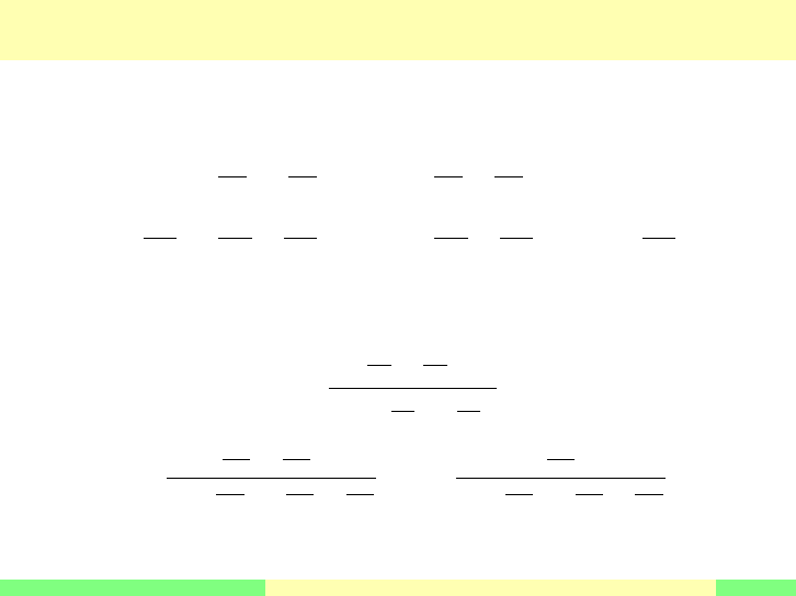
Constructing the Transfer Function: Suspension System
We isolate the z
1
and z
2
terms:
s
2
+
c
m
c
s +
K
1
m
c
ˆz
1
(s) =
K
1
m
c
+
c
m
c
s
ˆz
2
(s)
s
2
+
c
m
w
s +
K
1
m
w
+
K
2
m
w
ˆz
2
(s) =
K
1
m
w
+
c
m
w
s
ˆz
1
(s) −
K
2
m
w
ˆu(s)
ˆy(s) = ˆz
2
(s)
Which yields
ˆz
1
(s) =
K
1
m
c
+
c
m
c
s
s
2
+
c
m
c
s +
K
1
m
c
ˆz
2
(s)
ˆz
2
(s) =
K
1
m
w
+
c
m
w
s
s
2
+
c
m
w
s +
K
1
m
w
+
K
2
m
w
ˆz
1
(s) −
K
2
m
w
s
2
+
c
m
w
s +
K
1
m
w
+
K
2
m
w
ˆu(s)
M. Peet Lecture 6: Control Systems 11 / 23

Constructing the Transfer Function: Suspension System
Now we can plug in for ˆz
1
and solve for ˆz
2
:
ˆz
2
(s) =
K
2
(m
c
s
2
+ cs + K
1
)
m
c
m
w
s
4
+ c(m
w
+ m
c
)s
3
+ (K
1
m
c
+ K
1
m
w
+ K
2
m
c
)s
2
+ cK
2
s + K
1
K
2
ˆu(s)
Compare to the State-Space Representation:
d
dt
z
1
z
2
z
3
z
4
(t) =
0 1 0 0
−
K
1
m
c
−
c
m
c
K
1
m
c
c
m
c
0 0 0 1
K
1
m
w
c
m
w
−
K
1
m
w
+
K
2
m
w
−
c
m
w
z
1
z
2
z
3
z
4
(t) +
0
0
0
−
K
2
m
w
u(t)
y(t) =
1 0 0 0
0 0 1 0
z
1
z
2
z
3
z
4
(t) +
0
0
u(t)
M. Peet Lecture 6: Control Systems 12 / 23

Block Diagram Algebra
Series (Cascade) Interconnection
The interconnection of systems can be represent by block diagrams.
G
H
u
yy
1
Cascade of Systems: Suppose we have two systems: G and H.
Definition 2.
The Cascade or Series interconnection of two systems is
y
1
= Gu y = Hy
1
or
y = H(G(u))
M. Peet Lecture 6: Control Systems 13 / 23

Block Diagram Algebra
Series Connection (Cascade)
G(s)
H(s)
u(s)
y(s)y
1
(s)
H(s)G(s)
u(s)
y(s)
Series Interconnection:
•
The output of G is the input to H.
•
Let
ˆ
G(s) and
ˆ
H(s) be the transfer functions for G and H.
•
Then
ˆy
1
(s) =
ˆ
G
1
(s)ˆu(s) ˆy(s) =
ˆ
H(s)ˆy
1
(s) =
ˆ
H(s)
ˆ
G(s)ˆu(s)
•
The Transfer Function,
ˆ
T (s) for the combination of G and H is
ˆ
T (s) =
ˆ
H(s)
ˆ
G(s)
Note: The order of the
ˆ
G and
ˆ
H!
M. Peet Lecture 6: Control Systems 14 / 23


Block Diagrams
Parallel Connection
G(s)
H(s)
u(s)
y(s)
y
1
(s)
+
+
H(s)+G(s)
u(s)
y(s)
The Transfer function of a Parallel interconnection:
•
Laplace transform:
ˆy(s) = ˆy
1
(s) + ˆy
2
(s) =
ˆ
G(s)ˆu(s) +
ˆ
H(s)ˆu(s) =
ˆ
H(s) +
ˆ
G(s)
ˆu(s)
•
The Transfer Function,
ˆ
T (s) for the parallel interconnection of G and H is
ˆ
T (s) =
ˆ
H(s) +
ˆ
G(s)
M. Peet Lecture 6: Control Systems 16 / 23

Block Diagrams
Lower Feedback Interconnection
G(s)
K(s)
+
-
y(s)
u(s)
Feedback:
•
Controller: z = K(u − y) Plant: y = Gz
In the Frequency Domain:
ˆz(s) = −
ˆ
K(s)ˆy(s) +
ˆ
K(s)ˆu(s) ˆy(s) =
ˆ
G(s)ˆz(s)
so
ˆy(s) =
ˆ
G(s)ˆz(s) = −
ˆ
G(s)
ˆ
K(s)ˆy(s) +
ˆ
G(s)
ˆ
K(s)ˆu(s)
Solving for ˆy(s),
ˆy(s) =
ˆ
G(s)
ˆ
K(s)
1 +
ˆ
G(s)
ˆ
K(s)
ˆu(s)
M. Peet Lecture 6: Control Systems 17 / 23
Block Diagrams
Upper Feedback Interconnection (Regulators)
There is another Feedback
interconnection
•
u is the input
•
y is the output
ˆy(s) =
ˆ
G(s)ˆz(s)
ˆz(s) = u(s) −
ˆ
K(s)ˆy(s)
G(s)
K(s)
+
-
y(s)
u(s)
Which yields
ˆy(s) =
ˆ
G(s)
u(s) −
ˆ
K(s)ˆy(s)
=
ˆ
G(s)ˆu(s) −
ˆ
G(s)
ˆ
K(s)ˆy(s)
hence the Transfer Function is:
ˆy(s) =
ˆ
G(s)
1 +
ˆ
G(s)
ˆ
K(s)
ˆu(s).
M. Peet Lecture 6: Control Systems 18 / 23

The Effect of Feedback: Impulse Response
Inverted Pendulum Model
Transfer Function
ˆ
G(s) =
1
Js
2
−
Mgl
2
Controller: Static Gain:
ˆ
K(s) = K
Input: Impulse: ˆu(s) = 1.
Closed Loop: Lower Feedback
ˆy(s) =
ˆ
G(s)
ˆ
K(s)
1 +
ˆ
G(s)
ˆ
K(s)
ˆu(s) =
K
Js
2
−
Mgl
2
1 +
K
Js
2
−
Mgl
2
=
K
Js
2
−
Mgl
2
+ K
First Case:
•
If K >
Mgl
2
, then K −
Mgl
2
> 0, so
ˆy(s) =
K/J
s
2
+
K/J −
Mgl
2J
y(t) =
K
J
q
K/J −
Mgl
2J
sin
r
K/J −
Mgl
2J
t
!
0 2 4 6 8 10 12
−2.5
−2
−1.5
−1
−0.5
0
0.5
1
1.5
2
2.5
Impulse Response
Time (sec)
Amplitude
M. Peet Lecture 6: Control Systems 19 / 23

The Effect of Feedback: Impulse Response
Inverted Pendulum Model
0 5 10 15 20 25
0
2
4
6
8
10
12
14
16
18
x 10
6
Impulse Response
Time (sec)
Amplitude
Second Case:
•
If K <
Mgl
2
, then K −
Mgl
2
< 0, so
ˆy(s) =
K
J
1
s −
q
K/J −
Mgl
2J
+
1
s +
q
K/J −
Mgl
2J
y(t) =
K
J
e
√
K/J−
Mgl
2J
t
+ e
−
√
K/J−
Mgl
2J
t
Important: Value of K determines stability vs. instability
M. Peet Lecture 6: Control Systems 20 / 23

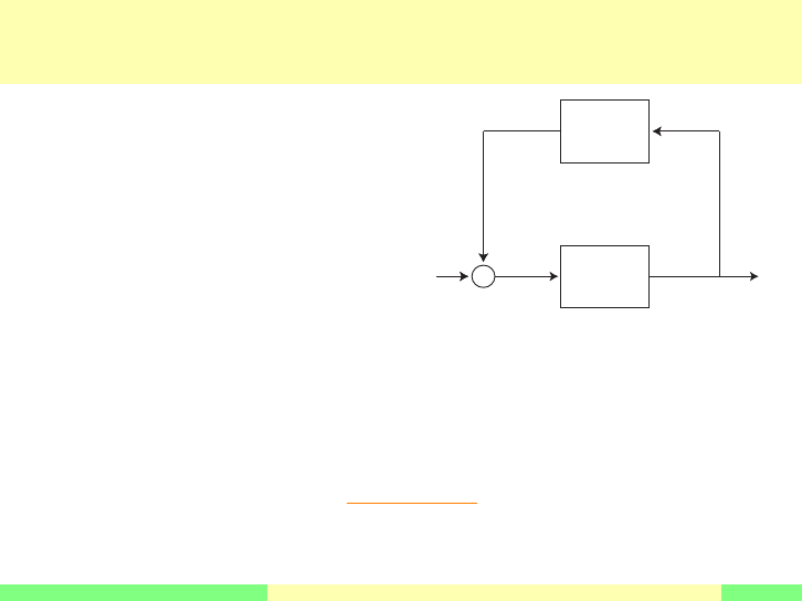
Block Diagrams
Reduction
Now lets look at how to reduce a more complicated interconnections
u(s)
y(s)
e(s)
-
+
-
+
1/s
1/s
K1
Label
•
The output from the inner loop z
•
The input to the inner loop u
First Close the Inner Loop using the Lower Feedback Interconnection.
ˆz(s) =
K
1
s
K
1
s
+ 1
ˆu(s) =
K
1
K
1
+ s
ˆu(s)
M. Peet Lecture 6: Control Systems 21 / 23


Summary
What have we learned today?
Transfer Functions
•
Transfer Function Representation of a System
•
State-Space to Transfer Function
•
Direct Calculation of Transfer Functions
Block Diagram Algebra
•
Modeling in the Frequency Domain
•
Reducing Block Diagrams
Next Lecture: Partial Fraction Expansion
M. Peet Lecture 6: Control Systems 23 / 23
