
Electrical Engineering Department
Dr. Ahmed Mustafa Hussein
Benha University
Faculty of Engineering at Shubra
1
Chapter Three: Block Diagram Dr. Ahmed Mustafa Hussein
Chapter # 3 Block Diagram
After completing this chapter, the students will be able to:
• Find the transfer function of electrical circuits,
• Reduce a block diagram of multiple subsystems to a single block representing
the transfer function from input to output (Block diagram algebra).
• Apply block-diagram algebra to Single Input Single Output (SISO), Multi
Input Single Output (MISO) and Multi Input Multi Output (MIMO) systems.
1. Introduction
In the previous chapter, we defined the Laplace transform and its inverse. We
presented the idea of the partial-fraction expansion and applied the concepts to the
solution of differential equations.
Consider a control system that shown in Fig. 1:
Fig. 1 Single, or multiple, block diagram representation

Electrical Engineering Department
Dr. Ahmed Mustafa Hussein
Benha University
Faculty of Engineering at Shubra
2
Chapter Three: Block Diagram Dr. Ahmed Mustafa Hussein
Now, we are ready to formulate the above system by establishing a viable definition
for a function that algebraically relates a system’s output to its input. Unlike the
differential equation, the function allows us to algebraically combine mathematical
representations of subsystems to yield a total system representation.
The transfer function can be represented as a block diagram, as shown in Fig. 2, with
the input R(s) to the left, the output C(s) to the right, and the system transfer function
G(s) inside the block.
Fig. 2 Single block diagram representation
Example (1):
Find the system Transfer function given by the following D.E.:
Taking the Laplace transform of both sides, assuming zero initial conditions, we have
Then the system Transfer Function G(s) is:
To obtain the system response C(s) at unit-step input R(s), then:
Expanding by partial fractions, we get
Finally, taking the inverse Laplace transform of each term yields
Transfer Function
G(s)
Input
R(s)
Output
C(s)

Electrical Engineering Department
Dr. Ahmed Mustafa Hussein
Benha University
Faculty of Engineering at Shubra
3
Chapter Three: Block Diagram Dr. Ahmed Mustafa Hussein
2. Transfer Function of Electric Circuits:
Consider the RLC circuit given in Fig. 3, find T.F. assuming the voltage V
c
is the
circuit output.
Fig. 3, RLC circuit
Using mesh analysis:
The circuit output V
c
(t) is given by
Then the circuit T.F. is given by:
Please refer to the table given below to simulate simple electric circuits

Electrical Engineering Department
Dr. Ahmed Mustafa Hussein
Benha University
Faculty of Engineering at Shubra
4
Chapter Three: Block Diagram Dr. Ahmed Mustafa Hussein
Example (2):
Consider a more complicated circuit as shown in Fig. 4. Find the T.F. I
2
(s)/V(s)
Fig. 4, RLC circuit
For Mech (1):
For Mech (2):
Using Cramer’s rule:

Electrical Engineering Department
Dr. Ahmed Mustafa Hussein
Benha University
Faculty of Engineering at Shubra
5
Chapter Three: Block Diagram Dr. Ahmed Mustafa Hussein
3. Operational Amplifiers (Op. Amp.)
For the operational amplifier, shown in Fig. 5, the differential input is v
2
-v
1
,
If v
2
is grounded, the amplifier is called inverting op. amp.
In circuit (a), the output V
o
is given by:
In circuit (b), the T.F. is given by:
Fig. 5, Inverting Op. Amp.
Example (3):
Find the T.F. for the Op. Amp. Circuit shown in Fig. 6.
Fig. 6, Op. Amp. circuit

Electrical Engineering Department
Dr. Ahmed Mustafa Hussein
Benha University
Faculty of Engineering at Shubra
6
Chapter Three: Block Diagram Dr. Ahmed Mustafa Hussein
For Non-inverting op. amp., shown in Fig. 7, the T.F. is given by:
Fig. 7, Non-Inverting Op. Amp.
Example (4):
For the non-inverting Op. Amp. given in Fig. 8, find the circuit T.F.
Fig. 8, Non-Inverting Op. Amp.

Electrical Engineering Department
Dr. Ahmed Mustafa Hussein
Benha University
Faculty of Engineering at Shubra
7
Chapter Three: Block Diagram Dr. Ahmed Mustafa Hussein
In general, the block diagram consists of blocks, arrows, take (pick) off points and/or
summing points. Fig. 9 shows these elements of the block diagram.
Fig. 9, Basic elements of block diagram
4. Terminology
Fig. 9, Block diagram components
Regarding the closed-loop control system shown in Fig. 9, we can define the
following terms;
Plant: A physical object to be controlled. The Plant G
3
(s), is the controlled system,
of which a particular quantity or condition is to be controlled.
Feedback Control System (Closed
loop Control System): A system which compares
output to some reference input and keeps output as close as possible to this reference.
Open
loop Control System: Output of the system is not feedback to the system.
Control Element G
2
(s), also called the controller, are the components required to
generate the appropriate control signal M (s) applied to the plant

Electrical Engineering Department
Dr. Ahmed Mustafa Hussein
Benha University
Faculty of Engineering at Shubra
8
Chapter Three: Block Diagram Dr. Ahmed Mustafa Hussein
Feedback Element H(s) is the component required to establish the functional
relationship between the primary feedback signal B (s) and the controlled output C(s).
Reference Input R (s) is an external signal applied to a feedback control system in
order to command a specified action of the plant. It often represents ideal plant output
behavior.
Controlled Output C(s) is that quantity or condition of the plant which is controlled
Actuating Signal E(s), also called the error or control action, is the algebraic sum
consisting of the reference input R (s) plus or minus (usually minus) the primary
feedback B (s).
Manipulated Variable M (s) (control signal) is that quantity or condition which the
control elements G
2
(s) apply to the plant G
3
(s).
Forward Path is the path from the actuating signal E(s) to the output C(s).
Feedback Path is the path from the output C(s) to the feedback signal B(s).
Summing Point: A circle with a cross is the symbol that indicates a summing point.
The (+) or (−) sign at each arrowhead indicates whether that signal is to be added or
subtracted.
Branch (pick/take off) Point: A branch point is a point from which the signal from a
block goes concurrently to other blocks or summing points.
We can conclude the above information by the following definitions:
According to the control system shown in Fig 10;
Fig. 10, Block diagram of a closedloop system with a feedback element.
Electrical Engineering Department
Dr. Ahmed Mustafa Hussein
Benha University
Faculty of Engineering at Shubra
9
Chapter Three: Block Diagram Dr. Ahmed Mustafa Hussein
5. Block Diagrams & Their Simplification
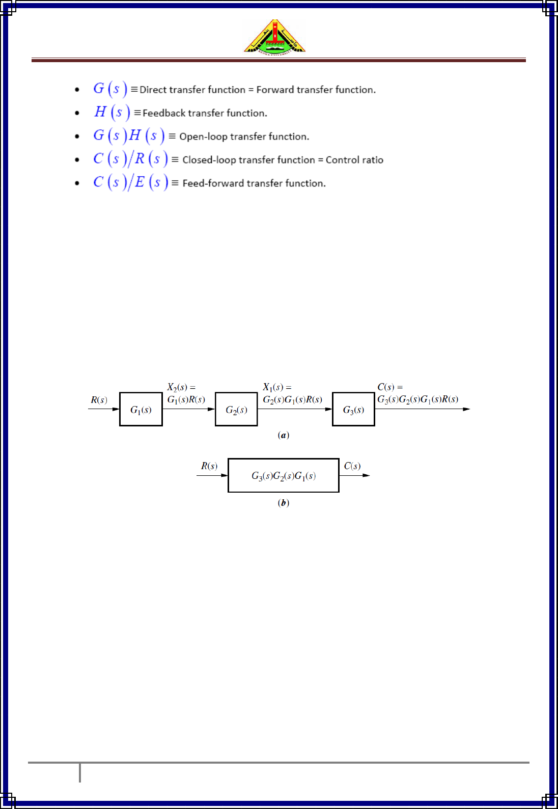
5.1 Cascade (Series) Connection
Figure 11(a) shows an example of cascaded subsystems. Intermediate signal values
are shown at the output of each subsystem. Each signal is derived from the product of
the input times the transfer function. The equivalent transfer function shown in Fig.
11(b), is the output Laplace transform divided by the input Laplace which is the
product of the subsystems’ transfer functions.
Fig. 11, (a) Original Block Diagram (b) Equivalent Block Diagram
5.2 Parallel Connection
Figure 12 (a) shows an example of parallel subsystems. Again, by writing the
output of each subsystem, we can find the equivalent transfer function. Parallel
subsystems have a common input and an output formed by the algebraic sum of
the outputs from all of the subsystems. The equivalent transfer function is given in
Fig. 12(b):

Electrical Engineering Department
Dr. Ahmed Mustafa Hussein
Benha University
Faculty of Engineering at Shubra
10
Chapter Three: Block Diagram Dr. Ahmed Mustafa Hussein
Fig. 12, (a) Original Block Diagram (b) Equivalent Block Diagram
5.3 Feedback Connections
The third connection is the feedback form as shown in Fig. 13 (a). The feedback
forms the basis for our study of control systems engineering.
We know that C(s) =G(s) E(s) & B(s) = H(s)C(s)
Where E (s) =R(s) B(s) = R(s) H(s)C(s)
Eliminating E(s) from these equations gives
C(s) = G(s) [R(s) H(s)C(s)] This can be written in the form
[1± G(s) H (s)] C(s) = G(s) R(s)
The equivalent transfer function is given in Fig. 13(b):
Fig. 13, (a) Feedback connection (b) Equivalent block
The Characteristic equation of the system is defined as an equation obtained by
setting the denominator polynomial of the transfer function to zero. The
Characteristic equation for the above system is:

Electrical Engineering Department
Dr. Ahmed Mustafa Hussein
Benha University
Faculty of Engineering at Shubra
11
Chapter Three: Block Diagram Dr. Ahmed Mustafa Hussein
5.4 Moving Summing point to get known connection
Moving summing point and jump over a block in the direction of the forward path,
we must multiply with the jumped block.
Moving summing point and jump over a block in the direction of the feedback path,
we must divide by the jumped block.
5.5 Moving Pick/take off point to get known connection
Moving take off point and jump over a block in the direction of the forward path, we
must divide by the jumped block.
Moving take off point and jump over a block in the direction of the feedback path, we
must multiply with the jumped block.

Electrical Engineering Department
Dr. Ahmed Mustafa Hussein
Benha University
Faculty of Engineering at Shubra
12
Chapter Three: Block Diagram Dr. Ahmed Mustafa Hussein
6. Block Diagram Reduction Rules
In many practical situations, the block diagram of a Single InputSingle Output
(SISO), feedback control system may involve several feedback loops, summing
points and/or take off points. In principle, the block diagram of (SISO) closed loop
system, no matter how complicated it is, it can be reduced to the standard single loop
form (Canonical form) shown in Fig. 13. The basic approach to simplify a block
diagram can be summarized in the following Table;
1.
Combine all cascade blocks
2.
Combine all parallel blocks
3.
Eliminate all minor (interior) feedback loops
4.
Shift summing points to left
5.
Shift take off points to the right
6.
Repeat Steps 1 to 5 until the canonical form is obtained
6.1. Some Basic Rules with Block Diagram Transformation

Electrical Engineering Department
Dr. Ahmed Mustafa Hussein
Benha University
Faculty of Engineering at Shubra
13
Chapter Three: Block Diagram Dr. Ahmed Mustafa Hussein
Example (5):
Example (6):
Reduce the given block diagram to a single block form.

Electrical Engineering Department
Dr. Ahmed Mustafa Hussein
Benha University
Faculty of Engineering at Shubra
14
Chapter Three: Block Diagram Dr. Ahmed Mustafa Hussein
Example (7):
The main problem here is the feedforward of V3(s). Solution is to move this pickoff
point forward.

Electrical Engineering Department
Dr. Ahmed Mustafa Hussein
Benha University
Faculty of Engineering at Shubra
15
Chapter Three: Block Diagram Dr. Ahmed Mustafa Hussein
Example (8):
Electrical Engineering Department
Dr. Ahmed Mustafa Hussein
Benha University
Faculty of Engineering at Shubra
16
Chapter Three: Block Diagram Dr. Ahmed Mustafa Hussein
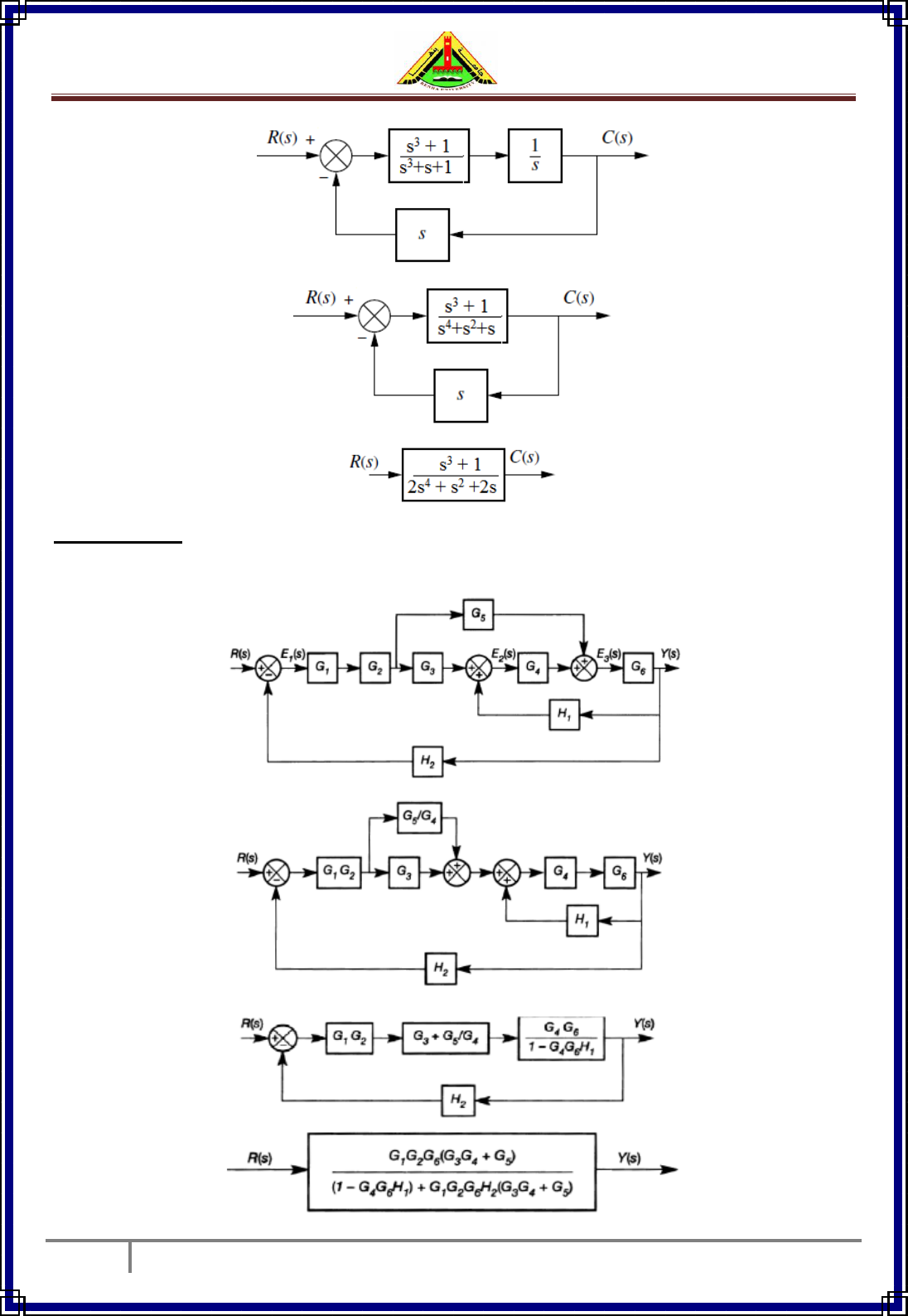
Example (9):
Use block diagram reduction to simplify the block diagram below into a single block
relating Y(s) to R(s).

Electrical Engineering Department
Dr. Ahmed Mustafa Hussein
Benha University
Faculty of Engineering at Shubra
17
Chapter Three: Block Diagram Dr. Ahmed Mustafa Hussein
7. MultipleInputs cases
In feedback control system, we often encounter multiple inputs to represent a
disturbance or something else. For a linear system, we can apply the superposition
principle to solve this type of problems, i.e. to treat each input one at a time while
setting all other inputs to zeros, and then algebraically add all the outputs as follows:
1.
Set all inputs to zero except one
2.
Transform the block diagram to solvable form
3.
Find the output response due to the chosen input action alone
4.
Repeat Steps 1 to 3 for each of the remaining inputs
5.
Algebraically sum all the output responses obtained in Step 3
Example (10): Determine the output C(S) of the following system
Using the superposition principle, the procedure is illustrated in the following steps:
Step1: Put D(s) ≡ 0 as shown in Fig. (a).
Step2: Reduce The block diagrams to the
block shown in Fig. (b)
Step 3: The output C
R
due to input R(s) is
shown in Fig. (c) and is given by the
relationship

Electrical Engineering Department
Dr. Ahmed Mustafa Hussein
Benha University
Faculty of Engineering at Shubra
18
Chapter Three: Block Diagram Dr. Ahmed Mustafa Hussein
Step 4: Put R(s) ≡ 0 as shown in Fig. (d).
Step 5: Put 1 into a block, representing the
negative feedback effect as shown in Fig. (d)
Step 6: Rearrange the block diagrams as
shown in Fig. (e).
Step 7: Let the 1 block be absorbed into the
summing point as shown in Fig. (f).
Step 8: The output C
D
due to input D(S) is :
The total output is C:
C(s) = C
R
+ C
D
Example (11):
Find the output C(S) of the control system shown below.
For Input R
1
:
For input R
2
:

Electrical Engineering Department
Dr. Ahmed Mustafa Hussein
Benha University
Faculty of Engineering at Shubra
19
Chapter Three: Block Diagram Dr. Ahmed Mustafa Hussein
Example (12):

Electrical Engineering Department
Dr. Ahmed Mustafa Hussein
Benha University
Faculty of Engineering at Shubra
20
Chapter Three: Block Diagram Dr. Ahmed Mustafa Hussein
Example (13):
For the closed-loop control system shown below,
a) Using block diagram algebra, find the system transfer function C(S)/R(S).
b) Obtain the system characteristic equation.
The blocks 12 & 5/(S+8) are cascade
The blocks 60/(S+8) & 3/20 are canonical
R(S)
+
C(S)
+
_
12
+
+
+
R(S)
+
C(S)
_
+
_

Electrical Engineering Department
Dr. Ahmed Mustafa Hussein
Benha University
Faculty of Engineering at Shubra
21
Chapter Three: Block Diagram Dr. Ahmed Mustafa Hussein
The blocks 60/(S+17) cascaded with 2/(S+T) and the result is canonical with 3/40
The system characteristic equation is
Rearrange the above equation to be:
R(S)
+
C(S)
_
_
R(S)
+
C(S)
_
R(S)
+
C(S)
_

Electrical Engineering Department
Dr. Ahmed Mustafa Hussein
Benha University
Faculty of Engineering at Shubra
22
Chapter Three: Block Diagram Dr. Ahmed Mustafa Hussein
Example (14):
If the control systems shown in Fig. A and B are equivalent, Find G
eq
.
Rearrange the block diagram as follows:
0.3
R(S)
C(S)
+
+
_
+
+
+
R(S)
_
+
C(S)
Fig. A
Fig. B
0.3
R(S)
C(S)
+
_
+
+
S
_
R(S)
C(S)
_
+
S+1
_

Electrical Engineering Department
Dr. Ahmed Mustafa Hussein
Benha University
Faculty of Engineering at Shubra
23
Chapter Three: Block Diagram Dr. Ahmed Mustafa Hussein
Add unity feedback with negative and positive sign
By comparing with the equivalent block diagram:
R(S)
C(S)
_
+
S+1
R(S)
C(S)
_
+
S+1
_
+
R(S)
C(S)
_
+
S
_
R(S)
C(S)
_
+
R(S)
_
+
C(S)

Electrical Engineering Department
Dr. Ahmed Mustafa Hussein
Benha University
Faculty of Engineering at Shubra
24
Chapter Three: Block Diagram Dr. Ahmed Mustafa Hussein
We get that
Example (15):
For the control system shown below, Calculate the transfer function C(s)/R(s)
The block diagram can be rearranged as:
K
0.3
R(S)
C(S)
_
+
0.4
_
_
R(S)
C(S)
_
+
_
0.4
R(S)
C(S)
_
+
K
0.3
R(S)
C(S)
+
+
_
+
0.4
+
+

Electrical Engineering Department
Dr. Ahmed Mustafa Hussein
Benha University
Faculty of Engineering at Shubra
25
Chapter Three: Block Diagram Dr. Ahmed Mustafa Hussein
Therefore, the closed loop T.F. is:
The system characteristic equation is given as:
Example (16):
For the control system shown below, Obtain the transfer function C(s)/R(s).
The blocks H1(S) and H2(S) are canonical and can be simplified as
The blocks G1(S) and G2(S) are cascaded and the result is canonical with
Example (17):
For the control system shown below, Obtain the transfer function C(s)/R(s) and
C(s)/D(s), then find an expression for the system response C(s).
R(S)
_
G1(S)
G2(S)
H1(S)
+
C(S)
+
H2(S)
_
R(S)
G1(S)
G2(S)
C(S)
+
_
G1(S)
R(S)
+
C(S)
+
_
G4(S)
G2(S)
G3(S)
H(S)
+
D(S)
+
+

Electrical Engineering Department
Dr. Ahmed Mustafa Hussein
Benha University
Faculty of Engineering at Shubra
26
Chapter Three: Block Diagram Dr. Ahmed Mustafa Hussein
Using super position
Assume R(S) = 0, and rearrange the block diagram as follows:
Now, assume D(S) = 0, rearrange the block diagram as follows
After moving the summing point as shown by the arrow indicated, the T.F. will be
From both T.F's we can obtain the expression for the system response C(s) as:
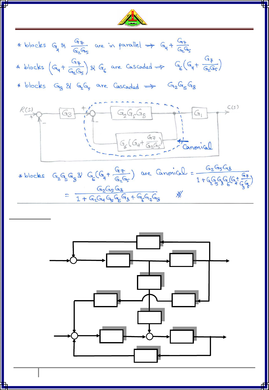
Example (18):
Simplify the block diagram shown below and then obtain the closed–loop transfer
function C(s)/R(s).
D(S)
+
C(S)
_
G2(S)
G3(S)
H(S)
G1(S)
G1(S)
R(S)
+
C(S)
_
G4(S)
G2(S)
G3(S)
H(S)
+
+

Electrical Engineering Department
Dr. Ahmed Mustafa Hussein
Benha University
Faculty of Engineering at Shubra
27
Chapter Three: Block Diagram Dr. Ahmed Mustafa Hussein
G7
G1
G6
G3
G2
G5
R(S)
C(S)
+
+
_
_
+
+
G4
G8
Electrical Engineering Department
Dr. Ahmed Mustafa Hussein
Benha University
Faculty of Engineering at Shubra
28
Chapter Three: Block Diagram Dr. Ahmed Mustafa Hussein
Example (19): For the Multi Input Multi Output (MIMO) control system shown below,
find the total value of C(S) and Y(S).
G1
(S)
R(S)
+
C(S)
+
_
+
+
G2
(S)
G3
(S)
H1
(S)
G5
(S)
G6
(S)
G7
(S)
G8
(S)
D(S)
_
Y(S)
H2
(S)
_
G4
(S)

Electrical Engineering Department
Dr. Ahmed Mustafa Hussein
Benha University
Faculty of Engineering at Shubra
29
Chapter Three: Block Diagram Dr. Ahmed Mustafa Hussein
Moving the take off point in the forward direction (divide by G2)
Also move the summing point in the feedback direction (divide by G7)
The obtained branch (G3G4/G2G7) is in parallel with G5G6
G1
(S)
R(S)
+
C(S)
+
_
+
+
G2
(S)
G3
(S)
H1
(S)
G5
(S)
G6
(S)
G7
(S)
G8
(S)
D(S)
_
Y(S)
H2
(S)
_
G4
(S)
G1 (S)
R(S)
+
C(S)
+
_
G2 (S)
H1 (S)
G7 (S)
G8 (S)
D(S)
_
Y(S)
H2 (S)
_

Electrical Engineering Department
Dr. Ahmed Mustafa Hussein
Benha University
Faculty of Engineering at Shubra
30
Chapter Three: Block Diagram Dr. Ahmed Mustafa Hussein
If Y(S) = 0
1) Let the input R(S) = 0
2) Let the input D(S) = 0
If C(S) = 0
3) Let the input R(S) = 0
4) Let the input D(S) = 0
Example (20):
For the control system shown below, find the value of K
1
, K
2
and K
3
if the system
transfer function is
R(S)
+
D(S)
+
Y(S)
C(S)
K
3
R(S)
C(S)
+
+
_
+
+
+
K
3

Electrical Engineering Department
Dr. Ahmed Mustafa Hussein
Benha University
Faculty of Engineering at Shubra
31
Chapter Three: Block Diagram Dr. Ahmed Mustafa Hussein
By Comparing:
As Check:
K
3
R(S)
C(S)
+
_
_
+
+
+
K
3
S
R(S)
C(S)
_
+
S+1

Electrical Engineering Department
Dr. Ahmed Mustafa Hussein
Benha University
Faculty of Engineering at Shubra
32
Chapter Three: Block Diagram Dr. Ahmed Mustafa Hussein
Example (21):
Find the system T.F.

Electrical Engineering Department
Dr. Ahmed Mustafa Hussein
Benha University
Faculty of Engineering at Shubra
33
Chapter Three: Block Diagram Dr. Ahmed Mustafa Hussein
Example (22):
Find the Transfer Function of the control system described by the block diagram
given below.
0.3
R(S)
Y(S)
+
+
_
+
_
+
+
+

Electrical Engineering Department
Dr. Ahmed Mustafa Hussein
Benha University
Faculty of Engineering at Shubra
34
Chapter Three: Block Diagram Dr. Ahmed Mustafa Hussein
Moving the summing point over the 1/S block
0.3
R(S)
Y(S)
+
+
_
+
+
+
Parallel
Feedback
_
+
0.3
R(S)
Y(S)
_
+
_
Cascade
Feedback
R(S)
Y(S)
_
+
Cascade
R(S)
Y(S)
_
+

Electrical Engineering Department
Dr. Ahmed Mustafa Hussein
Benha University
Faculty of Engineering at Shubra
35
Chapter Three: Block Diagram Dr. Ahmed Mustafa Hussein
Example (23):
Example (24):
Find the transfer function for the control system given below.

Electrical Engineering Department
Dr. Ahmed Mustafa Hussein
Benha University
Faculty of Engineering at Shubra
36
Chapter Three: Block Diagram Dr. Ahmed Mustafa Hussein

Electrical Engineering Department
Dr. Ahmed Mustafa Hussein
Benha University
Faculty of Engineering at Shubra
37
Chapter Three: Block Diagram Dr. Ahmed Mustafa Hussein
Example (25)
Consider the control system shown below, find the system transfer function.

Electrical Engineering Department
Dr. Ahmed Mustafa Hussein
Benha University
Faculty of Engineering at Shubra
38
Chapter Three: Block Diagram Dr. Ahmed Mustafa Hussein

Electrical Engineering Department
Dr. Ahmed Mustafa Hussein
Benha University
Faculty of Engineering at Shubra
39
Chapter Three: Block Diagram Dr. Ahmed Mustafa Hussein
Sheet 2 (Block Diagram)
Problem #1
Simplify the following control systems using block diagram algebra, and then find
the transfer function C(s) / R(s).
(a) (b)
c)
Problem #2
For the control system shown in Fig. (b) below,
a) Determine G(s) and H(s) that are equivalent to the block diagram of fig. (a)
b) Determine the transfer function C(s)/R(s)
R(S)
_
+
C(S)
+
_
G(s)
_
H(s)
R(S)
+
C(S)
(a)
(b)
Electrical Engineering Department
Dr. Ahmed Mustafa Hussein
Benha University
Faculty of Engineering at Shubra
40
Chapter Three: Block Diagram Dr. Ahmed Mustafa Hussein
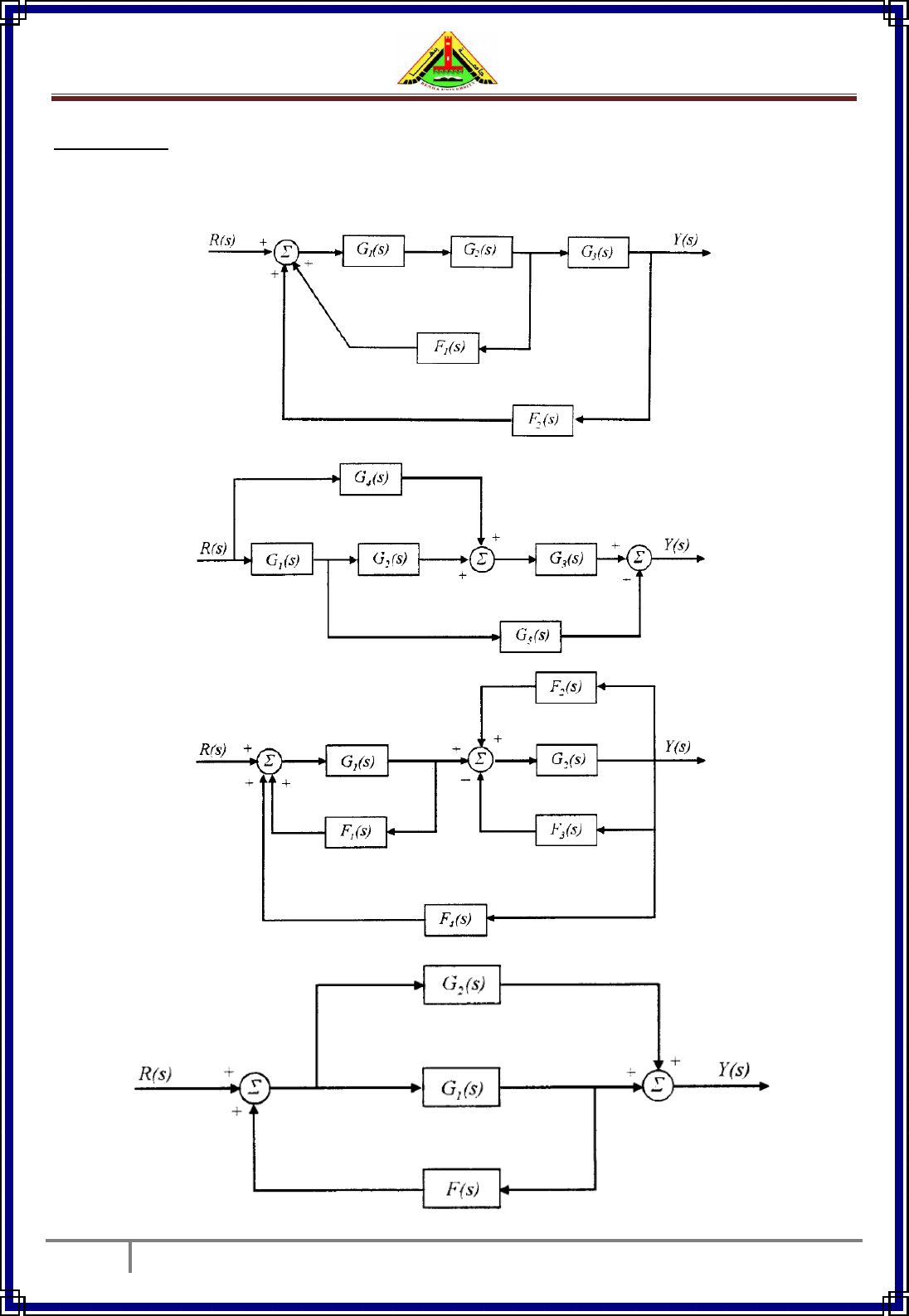
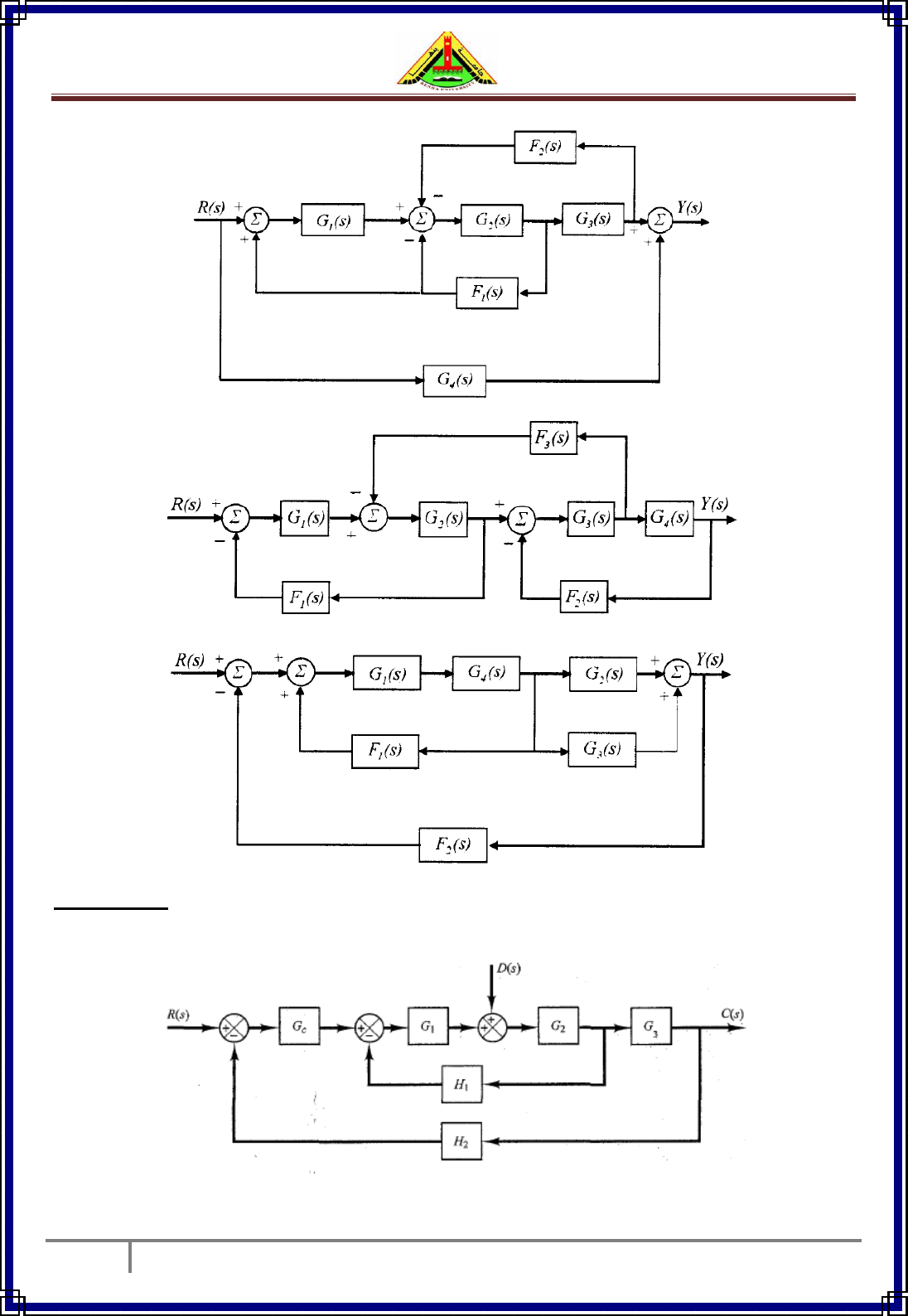
Problem #3
Simplify the following control systems using block diagram algebra, and then find
the transfer function Y(s) / R(s).
(a)
(b)
(c)
(d)
Electrical Engineering Department
Dr. Ahmed Mustafa Hussein
Benha University
Faculty of Engineering at Shubra
41
Chapter Three: Block Diagram Dr. Ahmed Mustafa Hussein
Problem #4
Obtain the transfer functions C(s)/R(s) and C(s)/D(s) of the systems shown below
(e)
(f)
(g)

Electrical Engineering Department
Dr. Ahmed Mustafa Hussein
Benha University
Faculty of Engineering at Shubra
42
Chapter Three: Block Diagram Dr. Ahmed Mustafa Hussein
Obtain the transfer functions Y(s)/R1(s) and Y(s)/R2(s) of the system shown below
Problem #5
The control system, shown in Fig. below, has two inputs and two outputs. Find
C
1
(s)/R
1
(s), C
1
(s)/R
2
(s), C
2
(s)/R
1
(s) and C
2
(s)/R
2
(s).
Problem #6
For the control system, shown in figure below, obtain the system transfer function.
R(S)
_
G1(S)
G2(S)
H1(S)
+
C(S)
+
H2(S)
_

Electrical Engineering Department
Dr. Ahmed Mustafa Hussein
Benha University
Faculty of Engineering at Shubra
43
Chapter Three: Block Diagram Dr. Ahmed Mustafa Hussein
Problem #7
For the control system shown below, find α, K, K1, K2 and K3 if Known that
Problem #8
Simplify the block diagram shown below and then obtain the closed–loop transfer
function C(s)/R(s).
K
K3
K2
K1
α
R(S)
C(S)
+
+
_
_
_
+
G7
G1
G6
G3
G2
G5
R(S)
C(S)
+
+
_
_
+
+
G4
G8

Electrical Engineering Department
Dr. Ahmed Mustafa Hussein
Benha University
Faculty of Engineering at Shubra
44
Chapter Three: Block Diagram Dr. Ahmed Mustafa Hussein
Problem #9
For the MIMO control system shown below, find the transfer matrix.
Problem #10
For the control systems shown below, find the transfer function.
R(s)
C(s)
G
1
(s)
G
2
(s)
G
3
(s)
G
4
(s)
H
1
(s)
H
2
(s)
+
+
+
+
_
_

Electrical Engineering Department
Dr. Ahmed Mustafa Hussein
Benha University
Faculty of Engineering at Shubra
45
Chapter Three: Block Diagram Dr. Ahmed Mustafa Hussein
References:
[1] Bosch, R. GmbH. Automotive Electrics and Automotive Electronics, 5th ed. John Wiley & Sons
Ltd., UK, 2007.
[2] Franklin, G. F., Powell, J. D., and Emami-Naeini, A. Feedback Control of Dynamic Systems.
Addison-Wesley, Reading, MA, 1986.
[3] Dorf, R. C. Modern Control Systems, 5th ed. Addison-Wesley, Reading, MA, 1989.
[4] Nise, N. S. Control System Engineering, 6th ed. John Wiley & Sons Ltd., UK, 2011.
[5] Ogata, K. Modern Control Engineering, 5th ed ed. Prentice Hall, Upper Saddle River, NJ, 2010.
[6] Kuo, B. C. Automatic Control Systems, 5th ed. Prentice Hall, Upper Saddle River, NJ, 1987.
