
Does Fiscal Policy Affect Interest Rates?
Evidence From A Factor-Augmented Panel
Salvatore Dell'Erba and Sergio Sola
WP/13/159

© 2013 International Monetary Fund WP/
IMF Working Paper
Fiscal Affairs Department
Does Fiscal Policy Affect Interest Rates? Evidence From A Factor-Augmented Panel
Prepared by Salvatore Dell’Erba and Sergio Sola
Authorized for distribution by Bernardin Akitoby
JuO\ 2013
Abstract
This paper reconsiders the effects of fiscal policy on long-term interest rates employing a
Factor Augmented Panel (FAP
) to control for the presence of common unobservable factors.
We construct a real-time dataset of macroeconomic and fiscal variables for a panel of OECD
countries for the period 1989-2012. We find that two global factors—the global monetary and
fiscal policy
stances—explain more than 60 percent of the variance in the long-term interest
rates. Compared to the estimates from models which do not account for global factors, we find
that the importance of domestic variables in explaining long-term interest rates is weakened.
Moreover, the propagation of global fiscal shocks is larger in economies characterized by
macroeconomic and institutional weaknesses.
JEL Classification Numbers: C10, E43, E62, F42, F62, H68.
Keywords:
Fiscal Policy; Interest rates; Real time data; Cross-sectional dependence;
Heterogeneous panels
Author’s E-Mail Address: [email protected]; [email protected]
This Working Paper should not be reported as representing the views of the IMF.
The views expressed in this Working Paper are those of the author(s) and do not necessarily
represent those of the IMF or IMF policy. Working Papers describe research in progress by the
author(s) and are published to elicit comments and to further debate.
2
Contents Page
I. Introduction ............................................................................................................................4
II. Literature Review ..................................................................................................................5
III. Data Description and Properties ..........................................................................................7
A. Data ...........................................................................................................................7
B. Properties ...................................................................................................................8
IV. Econometric Specification and Estimation Strategy ...........................................................8
A. The Econometric Model ............................................................................................9
B. Estimation Strategy .................................................................................................10
V. Estimation Results...............................................................................................................12
A. Baseline Model .......................................................................................................12
B. Time Variation in the Idiosyncratic Components ...................................................13
C. Discussion ...............................................................................................................13
VI. Effects of Global Shocks ...................................................................................................14
VII. Results From Different Specifications .............................................................................17
VIII. Robustness Checks ..........................................................................................................18
IX. Concluding Remarks .........................................................................................................20
Tables
1. Summary Statistics...............................................................................................................25
2. Cross Sectional Dependence Test ........................................................................................25
3. Panel Unit Root Tests ..........................................................................................................26
4. Principal Component Analysis ............................................................................................26
5. Baseline Estimation - Long-term Interest Rates ..................................................................27
6: Effects of Global Deficit Shock - Long-term Interest Rates ...............................................28
7. Baseline Estimation - Real Interest Rates and Sovereign Spreads ......................................29
8. Factors’ Interpretation - Long-Term Interest Rates .............................................................30
9. Cross Validation - Long-Term Interest Rates ......................................................................31
10. Baseline Estimation - Alternative Estimation Techniques: CCE-MG ...............................32
11. Non-Linearity with Crises - Long-Term Interest Rates .....................................................33
12. Non-Linearity with Public Debt - Long-Term Interest Rates ............................................34
13. Interpretation of the Global Factors - Long-term Interest Rates ........................................35
Figures
1. Long-Term Interest Rates 1989-2012 ..................................................................................36
2. Rolling Window Estimates – Long-Term Interest Rates .....................................................36
3. Country Specific Effects of an Increase in Global Deficit ..................................................37
4. Determinants of the Cross-Country Dispersion of the Effects of Global Deficit ................38
5. Global Factors and their Macroeconomic Interpretation .....................................................39
3
Appendices
A. Extraction of the Factors .....................................................................................................22
B. Variables..............................................................................................................................24
C. Tables and Figures ...............................................................................................................25
References ................................................................................................................................40

4
I. INTRODUCTION
1
The global financial crisis and its adverse effects on the budget deficits of advanced
economies have revived the debate on the link between fiscal policy and interest rates. The
strong convergence observed among advanced countries’ interest rates before the crisis came
to a halt when the global recession provoked a substantial deterioration of sovereigns’ fiscal
positions. Financial markets then suddenly started to discriminate between borrowers. These
developments seem to suggest that: (1) under increased capital market integration, interest
rates and risk premia tend to follow global factors rather than domestic variables; (2)
nonetheless, the effects stemming from fiscal policy can be large and substantial when
sovereigns face a common adverse budgetary shock. The objective of this paper is thus to
analyze the impact of fiscal policy on sovereign interest rates in a broad panel of OECD
countries, using a framework which can accommodate both the existence of common sources
of fluctuations as well as heterogeneous responses to global shocks. In particular, we want to
answer the following questions: In a context of high financial integration, do global factors
matter more than domestic factors? And how do global factors affect the cost of borrowing?
In this paper we consider the effects of fiscal policy on long-term interest rates. We follow
and expand the existing literature along two dimensions. Starting from the result according to
which the relationship between fiscal policy and interest rates becomes statistically
significant when using fiscal projections rather than actual data (Reinhart and Sack, 2000;
Canzoneri et al., 2002; Gale and Orszag, 2004; Laubach, 2009; Afonso, 2010) we construct a
real-time dataset based on macroeconomic projections collected from several vintages of the
OECD economic outlook. The use of real time data serves two different purposes: (i) it takes
into account the forward looking behavior of financial markets; (ii) it avoids the possible
reverse causality problem from interest rates to fiscal policy decisions which arise from the
use of actual data. Collecting fiscal projections from an independent agency like the OECD
rather than official government plans presents also a further advantage. As shown by
Beetsma and Giuliodori (2010) and Cimadomo (2008) governments’ released budget plans
tend to be overly optimistic in terms of expected fiscal outcome; on the other hand, the
forecasts released by an independent body such as the OECD are less prone to this
‘optimistic bias’.
Given the evidence of strong cross-country correlation in interest rates, we implement an
estimation method called Factor Augmented Panel (FAP)—originally developed by
Giannone and Lenza (2008)—which explicitly accounts for the presence of unobserved
global factors that affect interest rates simultaneously in all countries. By controlling for the
presence of global factors this method allows us to estimate the effects of the idiosyncratic
components of fiscal policy on interest rates. Moreover, it ensures unbiased estimates in case
the effects of global shocks are heterogeneous across countries. Finally, it has the desirable
property of allowing us to identify the global factors with observable data, and analyze the
1
The authors would like to thank, without implicating, Charles Wyplosz, Domenico Giannone, Alessan-
dro Missale and Ugo Panizza. We are also extremely grateful to Mark Watson, Manuel Arellano, Thomas Laubach,
Michele Lenza, Cedric Tille, Signe Krogstrup,Tommaso Trani, Lorenzo Forni, Emre Alper, Lone Christiansen,
Bernardin Akitoby, Adbelhak Senhadji and Carlo Cottarelli for helpful comments and suggestions. All remaining
errors are ours.
5
determinants of the cross-country differences of their effects on interest rates. Overall, we
find that using standard panel techniques provides results that are similar to those found in
previous literature. However, once we implement the FAP method to account for the
presence of global factors, we find that the estimated effect of budget deficits on long-term
interest rates becomes smaller in magnitude and insignificant, while the effect of public debt
remains significant and of about 1 basis points for a 1 percent increase in the debt to GDP
ratio.
The FAP technique also allows us to analyze in more detail the nature and the quantitative
importance of the common factors. Our results show that long-term interest rates are mainly
driven by two global factors, which explain more than 60 percent of their variance and can be
interpreted as the aggregate fiscal and monetary policy stances of the countries in the sample.
This suggests that the fiscal consolidations and the reductions of monetary policy rates which
took place almost simultaneously across advanced economies in the nineties can explain the
observed decline and convergence of long-term interest rates. However we also show that
long-term interest rates respond heterogeneously to the aggregate fiscal stance. In particular,
after an increase in the aggregate deficit long-term interest rates increase more in small
peripheral countries or countries characterized by a low initial level of financial integration,
and macroeconomic or institutional weaknesses.
The paper proceeds as follows. In Section II, we provide a brief review of the literature. In
Section III we discuss our dataset and its properties, which justify our estimation technique.
In Section IV we derive the estimating equations and explain the FAP methodology. In
Section V we present and discuss results. In Section VI we analyze the heterogeneity in the
country specific responses to global shocks, while in Section VII we report results from using
different specification. In Section VIII we do some robustness checks. Section IX concludes.
II. LITERATURE REVIEW
There is a vast empirical literature on the effects of fiscal policy on long-term interest rates
and sovereign spreads but, despite the large production, the results are still mixed. In spite of
the mixed results, we can identify few areas of consensus: (1) studies that employ measures
of expected rather than actual budget deficits as explanatory variables tend to find a
significant effect of fiscal policy on long-term interest rates (Feldstein, 1986; Reinhart and
Sack, 2000; Canzoneri et al. 2002; Thomas and Wu 2006; Laubach, 2009); (2) the effect of
public debt appears to be non-linear (Faini, 2006; Ardagna et al. 2007); (3) the effects of
public debt are quantitatively smaller than those of public deficit (Faini, 2006; Laubach,
2009); (4) the effects of global shocks and in particular “global fiscal policy” seem larger
than the effects of domestic shocks (Faini, 2006; Ardagna et al. 2007; Baldacci and Kumar
2010; Alper and Forni 2011); (5) as for sovereign spreads, they are found to respond strongly
to “global risk aversion” both in advanced countries (Codogno et al., 2003, Geyer et al.,
2004; Bernoth et al., 2004 and Favero et al., 2009) and in emerging markets (Gonzalez-
Rosada and Levy-Yeyati, 2008; Ciarlone et al., 2009).
This paper estimates the effects of fiscal policy on interest rates in panel of 17 OECD
countries. The papers more closely related to our work are Reinhart and Sack (2000), Chinn
and Frankel (2007), Ardagna et al. (2007). As Reinhart and Sack (2000) and Chinn and

6
Frankel (2007) we use fiscal projections instead of actual data. The choice of the regressors,
instead, closely follows Ardagna et al. (2007).
Reinhart and Sack (2000) estimate the effects of fiscal policy in a panel of 19 OECD
countries using annual fiscal projections from the OECD. They find that a one percentage
increase in the budget deficit to GDP increases interest rates by 9 basis points in the OECD
and by 12 basis points in the G7. The authors, however, do not consider the level of debt and
do not control for global factors. Chinn and Frankel (2007) focus on Germany, France, Italy
and Spain, while also considering evidence for UK, U.S. and Japan. They focus on the effect
of public debt and also use fiscal projections from the OECD. They find that the effect of
public debt is significant only when they include the US interest rate as a proxy for the
“world” interest rate. Ardagna et al. (2007) estimate the effects of fiscal policy in a panel of
16 OECD countries using yearly data, from 1960 to 2002, but do not use fiscal projections.
They find that a one percentage increase in the primary fiscal deficit to GDP increases long-
term interest rates by 10 basis points, a result similar to the one in Reinhart and Sack (2000).
Contrary to Reinhart and Sack (2000), Ardagna et al. (2007) also control for the level of debt,
finding evidence of non-linearity: interest rates increase if the level of debt to GDP is higher
than 60 percent. They also include cross-sectional averages of the fiscal variables to control
for the presence of global factors. They find that average debt and average deficit have
statistically significant effects on long-term interest rates, with magnitudes between 20 and
60 basis points.
Our main difference from the literature lies in the empirical strategy. We argue that to
properly identify the effects of fiscal policy we need a robust framework that allows us to
isolate idiosyncratic effects from common factors. While the previous literature has
acknowledged the relevance of global shocks as a driver of national interest rates, they have
constrained their effects to be homogeneous across countries. We show that this assumption
might lead to biased and inconsistent estimates. Our empirical model follows the insights of
recent literature that analyzes cross-sectional dependence in large panel. Cross-sectional
dependence
2
arises whenever the units of observations are simultaneously and
heterogeneously affected by common unobserved shocks. The recent econometric literature
provides different methodologies to deal with this type of structure in the data (Bai, 2009;
Pesaran, 2006). In this paper, we follow the methodology proposed originally by Giannone
and Lenza (2008) in their study of the Feldstein-Horioka puzzle. They show that the high
correlation between domestic savings and investments found in previous studies vanishes
once the panel takes into account global shocks with heterogeneous transmission. In Section
IV we provide a more detailed explanation of the methodology.
2
Following the terminology of Chudik, Pesaran and Tosetti (2011), we deal with strong instead of weak cross-
sectional dependence.

7
III. DATA DESCRIPTION AND PROPERTIES
A. Data
Our database contains real-time semi-annual forecasts of macroeconomic and fiscal variables
taken from the December and June issues of the OECD’s Economic Outlook, (EO), and
covering the period from 1989 to 2012. The countries included are 17: Australia, Austria,
Belgium, Canada, Denmark, Finland, France, Germany, Ireland, Italy, Japan, Norway,
Netherlands, Spain, Sweden, United Kingdom and United States.
In our dataset, the projected horizon of the forecast is always one year ahead. So for example,
for the June and the December issue of each year , we collect the projections for year 1.
3
The June and the December issues of the EO release forecasts with different information sets.
Following the terminology of Beetsma and Giuliodori (2008), the December issue contains a
forecast related to the planning phase of the budget law, while the June issue contains a
forecast related to its implementation phase. In spite of this difference, we pool them together
to achieve higher degrees of freedom. However we checked that splitting the sample
according to the June or December issue does not affect our main results.
4
As for the dependent variable we use the realized ten years yield on sovereign bonds
.
We construct this variable using the value of the interest rates observed in the month after the
release of the forecast: January for the December issue and July for the June issue. This
approach is useful because the forecasts on fiscal variables are likely to take into account
current market conditions and the level of interest rates. Under the assumption that financial
markets are forward looking and are able to incorporate rapidly all the available information,
sampling interest rates after the release of the forecasts reduces the issue of reverse causality.
Data on interest rates are taken from Datastream (Appendix B).
As indicators of fiscal stance, we use the expected primary deficit and the expected
public debt all measured as shares of previous period GDP.
5
We use primary the
deficit instead of total deficit to avoid the problem of reverse causality (since total deficit
contains also the total interest payments), while debt is measured as the total gross financial
liabilities of the general government.
6
Table 1 reports the descriptive statistics of the
variables of interest.
3
Starting from 1996, the OECD publishes also projections for year 2 in the December issue; for internal
consistency, we only keep the one year ahead projection.
4
Results are available upon request.
5
We also used current period GDP and trend GDP measured with a Hodrick-Prescott filter as a scaling variable
obtaining similar results.
6
A better measure could be the Net Financial Liabilities of the General Government. However, this measure is still
subject to substantial harmonization problems since it is not yet established how to compare the value of
governments’ assets across countries. An even better measure would include contingent liabilities. However, there is
an ever bigger issue on how to compare these items across countries. This is though an interesting area of future
research.

8
B. Properties
The importance of the cross-sectional correlation among our variables of interest can be
observed when looking at the behavior of long-term interest rates in our sample (Figure 1).
We have grouped the countries from the right in the following way: first are the
Scandinavian countries (Norway, Sweden, Denmark); then the EMU countries (Finland,
Ireland, Italy, Spain, Austria, Belgium, Netherlands, France, Germany); then the Anglo-
Saxon countries (Australia, Canada, the UK) and finally Japan and the U.S. Long-term
interest rates are higher at the beginning of the sample in all countries. Starting from 1994,
there appears to be a strong convergence, with an especially marked reduction of the interest
rates in the peripheral EMU countries (Ireland, Italy, Spain). Nevertheless, the convergence
is observed also outside the EMU. Interest rates remain low throughout the 2000 particularly
so in Japan, and they begin to diverge only during the crisis.
This evidence is in line with the hypothesis that countries might be subject to the same
shocks causing a co-movement in interest rates. To verify the importance of common factors,
we test for the presence of cross-sectional dependence in long-term interest rates and the
macroeconomic variables of interest using Pesaran's (2004) test. For a panel of N
countries, the test statistic is constructed from the combinations of estimated correlation
coefficients. Under the null of cross-sectional independence the statistic is distributed as a
standard Normal. For all the variables in our sample we find strong evidence of cross-
sectional dependence (Table 2).
7
We also conducted standard stationarity tests (Table 3). We first implement the Pesaran's
(2007) test for panel unit root and we find indication that almost all the variables can be
treated as stationary. There is mixed evidence with respect to the fiscal variables. We
therefore implement the Moon and Perron's test (2004) which accounts for multifactor
structure, which gives evidence of stationarity for all the variables.
8
We thus conclude that all
the variables in our panel can be treated as stationary.
IV. ECONOMETRIC SPECIFICATION AND ESTIMATION STRATEGY
In this section we describe the FAP technique and discuss its properties and estimation
procedure. We derive the estimating equation starting from a data generating process in
which a set of global unobservable factors simultaneously determine interest rates and
macroeconomic variables. This feature generates the pattern of cross-sectional dependence
7
This test is based on the following set of hypotheses:
:
,
0for
:
0forsome
Given the
estimated pairwise correlation coefficients of the residuals:
∑
∑
/
∑
/
Pesaran (2006) showed
that the following statistic:
∑∑
is distributed as a Standard Normal. The asymptotic
distribution of the test statistic is however developed for .
8
We were unable to implement the Pesaran, Smith and Yamagata (2008) test, given that our time series is too small.
9
observed in the data (see Section III). In the next section we discuss the econometric model
and show—as in Giannone and Lenza (2008)—that standard estimation techniques are likely
to yield biased estimates whenever the effects of global factors are truly heterogeneous
across countries. In Section IV.B we discuss the estimation of the unobserved factors and
refer the reader to Appendix A for more details.
A. The Econometric Model
Let
and
be respectively the long-term interest rate and a set of observable variables,
with 1,…,;1,…,. When looking for the determinants of interest rates the
natural starting point is a linear model of thetype:
(1)
where the country intercepts
capture time invariant heterogeneity across countries. This is
the equation estimated for example by Reinhart and Sack (2000) in a panel of 20 OECD
countries. The estimates of the coefficients are however unlikely to be informative of the
effect of
on
if these are simultaneously determined by a set of unobserved global
factors. This is the case for open and integrated economies where there exist common
sources of fluctuations - such as common business cycle shocks. A common shock would in
fact jointly determine the reaction of monetary and fiscal authorities across countries and
hence the level of interest rates. Following Giannone and Lenza (2008) we therefore assume
a factor structure of the type:
(2)
in which observable quantities
,
are a function of a set of unobservable global
factors
with heterogeneous impact in each country
,
, :1,...,.
Given this data generating process, an accurate estimate of the effect of macroeconomic and
fiscal policy variables on interest rates should be based on the idiosyncratic components
only:
(3)
Equation (3) cannot be estimated because the idiosyncratic components
,
are
unobservable, but we can use (2) to substitute the idiosyncratic component in (3) and rewrite
the equation in terms of observable quantities and global factors:
10
(4)
By taking explicitly into account the global factors
, (4) allows us to estimate the
relationship between the idiosyncratic components of the variables of interest.
Consistent estimates of the common factors, allow an estimation of the by standard panel
techniques. In Section 4.2 we show that these can be obtained extracting principal
components from the set of observable variables of equation
4
,
,
,...,;,...,
. This
estimation technique goes under the name of Factor Augmented Panel (FAP).
When the data generating process is represented by the system in (2), we can obtain unbiased
estimates of the coefficients only if we allow the factors to have heterogeneous impact
across countries (
). This aspect has been often ignored in previous studies. In fact,
when tackling the issue of common unobserved factors the literature has mainly pursued
different paths. The first approach (Chinn and Frankel, 2007) consists of finding an a priori
observable variable (or a subset of variables) which might affect contemporaneously the
interest rates across countries, and introduce it directly in the panel:
(5)
where the variable (
) is the vector (or matrix) of identified common factors. Alternatively,
unobserved factors have been accounted for by introducing time effects. This would lead to
the estimation of the following model (Ardagna et al. 2007):
(6)
This is equivalent to assuming that in each time period there is a common shock which
affects homogeneously countries’ interest rates.
Differently from the FAP specification in (4), equations (5) and (6) impose homogeneous
effects of the global factors, represented either by the common regressors
or by the time
effects
. If however the unobserved factors have truly a heterogeneous effect across
countries, then the country specific components will become part of the error terms of (5) and
(6). Therefore, if the factors are correlated with the observable variables—as implied by
(2)—equations (5) and (6) will suffer from endogeneity and produce biased estimates.
B. Estimation Strategy
To obtain consistent estimates of the sets of unobservable factors we follow Giannone and
Lenza (2008) and use principal components. This is a general procedure that can be applied
whenever in a linear regression the variables have a factor structure. It consists of taking the

11
entire set of dependent and independent variables for all the cross sections and, after
stacking them together in a single matrix, apply principal components.
Hence to estimate the unobserved factors of equation (4), we collect all the variables
,
,..,;,...
in a matrix
:
,...,
;
,...,
If the elements
have dimension , the matrix
will be of dimension
1
.
9
The Principal Component Analysis
of
produces set of
1
orthogonal
vectors which are the eigenvectors obtained from the eigenvalue-eigenvector decomposition
of the covariance matrix of
. The eigenvectors are linear combinations of the columns of
. However, under the assumptions that common factors are pervasive and that
idiosyncratic shocks are not pervasive, the eigenvectors are a consistent estimate of the
common factors, with consistency achieved as the dimensions of
increase. Of all the
1
eigenvectors extracted from
we keep the first , which are the ones associated
with the highest proportion of explained variance. This procedure ensures that the factors
are indeed those elements which explain the bulk of the correlation among all of our data
series and are therefore responsible for their observed co-movements.
The first two eigenvectors explain 68 percent of the panel variance with the third one
contributing for less than 10 percent (see Table 4).
Following Giannone and Lenza (2008), we therefore take into consideration only the first
two factors. Using these two estimated vectors we can rewrite equation (4) as:
(7)
Notice that, while we allow the response to the common factors
to vary across country,
we impose the coefficients to be common to keep the results consistent with those obtained
in previous studies. The economic interpretation of the estimated factors
and
is
important for the scope of our analysis. In Appendix A we show that these two elements can
be interpreted as the average monetary policy and the average fiscal policy stances of the
countries in our sample.
Although having estimated elements in the regression introduces a further source of
uncertainty, which normally requires to bootstrap the standard errors, we rely on the result by
Giannone and Lenza (2008), Bai (2004) and Bai and Ng (2006) who show that with a
relatively large number of countries there is no generated regressor problem.
10
9
See Appendix A for more details on the elements of
.
10
Bai (2003) and Bai and Ng (2006) show that factors can be treated as known if the number of countries is larger
than the square root of the sample size
.

12
The FAP is however not the only methodology proposed in the literature. Other types of
estimator developed to tackle the issue of common unobservable factors and cross-sectional
dependence are e Pesaran's (2006) Common Correlated Effect CCE, and Bai's (2009)
Interactive Fixed Effects (IFE). In Section VIII we show that our main results are preserved
if we employ these two alternative estimation techniques.
V. ESTIMATION RESULTS
A. Baseline Model
In this section we present the results from the estimation of equation (7). The set of
regressors
contains the OECD forecasts of public debt, primary deficit, real GDP growth.
We also include the expected short term interest rate
11
and the expected inflation rate - to net
out of the long-term interest rate the expectations on future monetary policy stance and the
inflation premium.
The results are reported in Table 5. In the table, columns 1 and 2 use standard panel
techniques, while column 3 presents the results of the FAP estimation. In particular, we first
estimate equation (7) using only country fixed effects
(column 1-FE), then we include also
time fixed effects
(column 2-2FE) and finally we include both fixed effects and estimated
factors (column 3-FAP).
12
At the bottom of each table we include, as a further specification test, the value of the CSD
statistic, which is Pesaran's (2006) test for cross-sectional dependence
13
applied to the
residuals of the estimated equation.
Our results show that the positive correlation between fiscal variables and long-term interest
rates previously found in the literature is not robust to the introduction of general equilibrium
effects. A standard FE estimator shows that a one percentage point increase in the expected
primary deficit to GDP ratio increases interest rates by around 9.8 basis points, while a 1
percent increase in the expected debt to GDP ratio increases interest rates by around 1.3 basis
points (column 1). However, the large value of the CSD statistic (43.51) for the residual,
indicates that the regression is misspecified.
Looking at columns 2 and 3 we first notice the importance of accounting for common factors.
For both estimators, the CSD statistic falls markedly compared to the FE, but the FAP
performs better against the 2FE (-1.80 vs. -0.87). The response of long-term interest rates to
11
We also tried using the actual 3 months interest rate from Datastream obtaining very similar results.
12
The country and time fixed effects are eliminated by means of a standard within transformation applied to the left
hand side and observable right hand side variables - See Bai (2009).
13
We report the value of the statistic instead of the p-value because the asymptotic for this test is developed for
and to our knowledge there is no test of residual cross-sectional dependence which does not rely on this assumption.
Hence, because in our panel we have we prefer to report the value of the statistic and interpret the changes in
its values across different specifications as the marginal impact of the introduction of common factors in correcting
cross-sectional dependence.

13
idiosyncratic factors diminishes in both cases. When we allow for heterogeneous response to
global shocks with the FAP (column 3) primary deficit becomes statistically insignificant,
while the effect of public debt becomes significant. As for the magnitude, the effect is similar
to the standard FE estimator (column 1): a 1 percent increase in public debt increases long-
term interest rates by 1.3 basis points. The coefficient on the short-term interest rate also
decreases significantly when using the FAP, indicating that, accounting for general
equilibrium effects, long-term interest rates are less responsive to domestic monetary policy.
The coefficient on GDP growth is negatively signed but the effect is insignificant. Finally,
we find a positive but not significant relation with expected inflation.
B. Time Variation in the Idiosyncratic Components
In this section we check whether the importance of the idiosyncratic components has been
changing over time. We expect that, with the progressive financial and economic integration
among advanced economies, global factors become more important and thus reduce the
impact of idiosyncratic policies. We are primarily interested in the time varying effect of
public debt and primary deficits. However we also analyze the coefficient on the short term
interest rate, to assess whether financial integration affects the sensitivity to own monetary
policy as suggested by the results presented in the previous section. We re-estimate (7) using
rolling regressions with a window of 24 periods.
14
We can therefore follow the evolution
over time of the coefficients on primary deficit, public debt and short-term interest rates
(Figure 2).
As expected, there is a clear downward trend in the coefficients, indicating a progressive loss
of importance of domestic policy variables. This is the case for both fiscal and monetary
policy. The coefficient on the short term interest rate shows that central banks have been
progressively losing effectiveness in stirring long-term rates. This evidence is consistent with
that presented by Giannone et al (2009), who show how in the recent decades long-term
interest rates have become more disconnected from country-specific monetary policy stances.
The importance of idiosyncratic fiscal factors stays flat for most of the sample and then
increases for the last period. While fiscal deficits do not have any impact through the more
recent period, the coefficient on public debt increases but the uncertainties around its
estimates also increases due to the large variation observed in debt during this period. This
evidence suggests a possible repricing of risk in the aftermath of the global financial crisis
(see Sgherri and Zoli (2009) and Poghosyan (2012) for evidence on the EMU).
15
C. Discussion
The results so far indicate that, when we account for heterogeneous response to global
shocks: (1) long-term interest rates remain positively related only to public debt; (2) there is
14
Having 49 time periods, the size of the window is determined by having an equal split of the sample in the first
regression.
15
A stronger evidence of increase in the importance of the idiosyncratic components of debt and deficit is visible
when looking at sovereign risk rather than long-term interest rates. See Dell’Erba and Sola (2013).

14
mild evidence of increased importance of idiosyncratic fiscal policy in the last crisis. Our
results stand partly in contrast with previous literature. In particular, past studies have found
a significant effect of public deficits on long-term interest rates (Ardagna et al. (2007)). The
effect of public debt on long-term interest rates is also smaller compared to previous
estimates. Laubach (2009) for example, finds that a 1 percent increase in public debt to GDP
leads to an increase in long-term interest rates by 3 to 4 basis points, while we find that the
effects are less than 1 basis point. While our results cannot be strictly comparable due to
differences in the sample and in the data, we argue that our results are consistent with the
implications of standard neoclassical models if we change the assumption on the degree of
crowding-out. Laubach (2009) shows that, within the neoclassical growth model, under the
assumption that roughly two-thirds of the increase in public debt is offset by domestic
savings, a 1 percent increase in public debt to GDP leads to an increase in real interest rates
by 2.1 basis points.
16
However, recent evidence on the Feldstein-Horioka regression by
Giannone and Lenza (2008), show that less than one-fifth of savings in developed countries
are retained for domestic investment. This evidence on the lower degree of crowding-out
reconcile our estimates with theory, and generate effects of public debt on real interest rates
in the range of 1 basis points (Table 5, Column 3).
17
VI. EFFECTS OF GLOBAL SHOCKS
The fact that, after accounting for global factors, the idiosyncratic component of fiscal policy
plays a smaller role compared with earlier literature does not necessarily mean that fiscal
policy is unimportant. We have seen so far that nominal interest rates are driven by factors
which closely resemble global monetary and global fiscal policy stances. In this section we
use the FAP estimator to focus on how shocks to the aggregate fiscal stance transmit to
domestic long-term rates. In terms of our estimating equations, we analyze the magnitude
and the cross-country differences in the coefficients
in equation (7).
This exercise can help to shed some light on the dynamics of the interest rates observed
during the recent crisis, which was characterized by a simultaneous increase in advanced
countries’ budget deficits. From a theoretical point of view, in a group of financially
integrated economies a shock in the global fiscal stance will affect countries’ interest rates
through its effect on the ‘world interest rate.’ If all governments increase spending together,
this affects the aggregate savings schedule whenever governments’ actions are not perfectly
compensated by an equal and opposite reaction from the private sector. Therefore the
equilibrium ‘world interest rate’ increases and, because of capital markets integration,
interest rates in all countries adjust accordingly.
The existing literature has already recognized the importance of these global effects. Faini
(2006) for example, analyzes the effect of a ‘global fiscal expansion’ for EMU countries;
Ardagna et al. (2007) extend their sample to the OECD while Claeys et al. (2008) used a
16
Following the discussion in Laubach (2009) , the effect of 1 percent increase in public debt to GDP on interest rates
is given by the formula: 1/
where s=0.33 is the capital share on national income; k=2.5 is the capital-
output ration; c=0.6 is the degree of crowding out.
17
Assuming the parameter is c=0.2 the estimated effect is 0.7 basis points.

15
panel of 100 countries. Similarly, Alper and Forni (2011) used a panel of advanced and
emerging countries. In all cases, the effects are found to be statistically significant and much
larger than those of domestic fiscal shocks.
18
One important advantage of our approach is that
we can analyze not only the relative magnitudes of the effects of idiosyncratic versus global
shocks, but we can also study how the effects of global shocks differ across the countries in
our sample. For instance, when global deficits increase we would expect interest rates to
respond more in countries with relatively closer capital account, as they can only draw from
the smaller pool of national savings instead that from the world market. Alternatively,
interest rates might increase more in countries with large macroeconomic or fiscal
vulnerabilities.
To estimate the effects of these global factors we re-estimate equations (7) replacing the
estimated factors with their economic interpretation. As discussed in Appendix A we use the
average expected primary deficit
19
and the average expected short term rate of the countries
in our sample. The estimated effects of a fiscal increase in global deficit are indeed
quantitatively important and highly heterogeneous across countries (see Table 6 and Figure
3).
There seems to be a clustering of countries, with Ireland, Italy and Spain displaying the
highest coefficients. For them, a one percentage point increase in average deficit increases
nominal interest rates between 43 and 51 basis points. Positive effects are also observed for
the group of the core EMU members (Austria, Belgium, Netherlands, France), the Nordic
countries (Finland, Denmark, Sweden), and the Anglo-Saxons (UK and Australia). For these
groups, however, the coefficients are about 50 percent smaller, ranging between 10 and 25
basis points, with Finland displaying the highest coefficient. The group of countries for
which the estimated coefficients are the lowest is composed of the U.S., Norway and
Germany, for which they are also not statistically significant. These are countries that are
either relatively “large” (U.S., and Germany) and – at least in the case of the U.S. - more
likely to behave as closed economies; or for which availability of capital is more driven by
the exogenous variation in the price of oil and natural gas (Norway). Quantitatively, average
deficit is by far more important than the idiosyncratic fiscal components. Its average effect is
in fact around 20 basis points, which is more than ten times larger than the effect of an
increase in idiosyncratic primary deficit. A one standard deviation in the increase in global
fiscal stance can have effects as large as 1 percentage point.
18
Faini (2006) finds that the effects on interest rates of domestic fiscal policy shocks are rather small compared to
those caused by a global fiscal expansion: a change in domestic surplus leads to a 5 basis points reduction of interest
rates, while a change in the EMU surplus leads to a 41 basis points decrease in interest rates. Ardagna et al. (2007)
obtain similar results for the OECD. They analyze the world fiscal stance as both the aggregate primary deficit and
the aggregate debt. They find that, depending on the specification, the world deficit leads to increase in interest rates
between 28 and 66 basis points, while world debt increases interest rates between 3 and 21 basis points. In both
papers, the effects of global shocks are supposed to be homogeneous across countries.
19
The theory would suggest to use the world fiscal stance as control. Here, we use instead the average fiscal stance in
17 advanced economies. We believe this provides a reasonable approximation (see also Ardagne et al. (2007) on the
point).

16
Besides recognizing the quantitative importance of the effects of global fiscal stance, our
framework allows us to investigate the driving factors behind their cross-sectional dispersion.
Our evidence shows that there exists a relationship between the estimated coefficients and:
(i) the initial level of capital markets integration, measured by the initial level of the long-
term interest rate, or the initial level of the Chinn and Ito Index
20
(top left and bottom left
panels of Figure 4); (ii) the size of the current account imbalances (top right panel of Figure
4) and (iii) an indicator of fiscal and political risk (bottom right panel of Figure 4).
This descriptive evidence provides an interesting explanation of the behavior of long-term
interest rates in the recent decades. The progressive fiscal retrenchment which took place
among industrialized countries at the beginning of the nineties, by increasing aggregate
savings, has caused long-term interest rates to decline. This movement has been facilitated by
the progressive economic and especially financial integration which, consistently with
theoretical models, has induced interest rates to converge to the “world interest rate.” The
convergence forces have obviously influenced more those countries which were
characterized by low initial financial integration.
21
In these countries, however, the
compression of long-term interest rates went hand in hand with the build-up of large external
imbalances, which eventually caused larger increases in interest rates as soon as the global
deficit started expanding. The drain of savings caused by the global fiscal expansion
experienced since the onset of the crisis has in fact put upward pressure to the “world interest
rate,” and as a result of higher need for savings, investors have repatriate capital from abroad,
making capital scarcer in countries with large current account deficits (see Arslanap and
Tsuda 2012).
22
Finally, the increase in long-term interest rates can also be associated with an increase in risk
premia. Hence, we would expect that, as capital becomes scarcer due to the expansion in
global deficit, countries with weak institutions or weak fiscal positions would suffer
proportionately more. In the bottom panel of Figure 4 we show that the dispersion in the
country-specific effect global fiscal policy is positively related with an indicator of fiscal and
political vulnerability. This indicator has been constructed as the simple average of the
20
Chinn and Ito (2009).
21
While the Chinn and Ito (2009) index measures de Jure financial integration, the level of long-term nominal interest
rates can be interpreted as a measure of de Facto financial integration.
22
In terms of our theoretical model - equation (4) - the responsiveness of the domestic interest rates to the global
factors are given by
. This means that they are directly proportional to the responsiveness of the
domestic interest rates to the global factors and inversely related to the responsiveness of the regressors
. A close
capital account translates into a higher value of the coefficients
because an expansion of aggregate budget deficits
would mean relatively higher excess demand of capital for countries that can only access their domestic capital
markets. A large share of foreign capital, instead, can translate again into high values of the
coefficients. If in fact
global fiscal expansions take place in periods of recessions when investors also pull out capital from abroad, then
running a high current account deficit might aggravate capital scarcity and induce higher increase in interest rates.

17
countries’ debt to GDP ratio and the index of political risk constructed by the International
Country Risk Guide.
23
Overall, these results give us a key of interpretation for the observed behavior of interest
rates in the recent decades. The common move of the governments of most advanced
countries towards fiscal discipline has played a major role in explaining the convergence of
long-term interest rates. The excess savings generated by fiscal retrenchment, however, in
some countries contributed to create macroeconomic and fiscal vulnerabilities which
eventually stroke back as the global deficit began to increase during the financial crisis
(Giavazzi and Spaventa 2010).
VII. RESULTS FROM DIFFERENT SPECIFICATIONS
In this section we report the results from using different left-hand side variables. We first
measure the impact of fiscal policy on the real interest rate. Since the ex-ante real long term
yield is unobservable, as in Ardagna et al. (2007) we construct it from the data. Since the
Outlook provides forecast only for inflation in period t+1, we proxy inflation expectations in
t+10 with the “trend inflation” calculated with the help of a Kalman Filter applied recursively
on the series of inflation expectations for the year t+1. As a second exercise, we measure the
impact of fiscal policy on the yield spreads measured as the difference between the ten years
yield and the yield on a risk-free asset of the same maturity
).
24
To correct for the
presence of exchange rate risk, we follow Codogno et al. (2003) and before computing the
spreads we subtract from the long-term interest rates the yield on the interest rate swaps of
the same maturity. However, because of the availability of data on interest rate swaps, the
sample covers the period 1997-2012.
Before estimating the FAP equations for the real interest rate and the spreads equation we
have to re-estimate the global factors for each of these two specifications. In the first case the
results are very similar to the ones obtained for the equation for long-term nominal rates: two
global factors account for more than two thirds of the variance and they can be interpreted as
the global monetary and the global fiscal policy stances. For the spreads equation, instead,
the relevant factors seem to be three: besides global monetary and fiscal policy stances a
third factor which mimics global risk aversion is very relevant.
25
More details on the
23
To make the debt to GDP ratio and the political instability index comparable with each other, they have been first
standardized to have zero mean and unit variance.
24
To measure the yield spreads we need to define a benchmark. In general the literature on EMU countries uses the
interest rate on German government Bunds as a benchmark. After the introduction of the common currency, the
exchange rate risk among EMU countries has disappeared and Germany has acquired the “status” of safe haven (see
von Hagen et al. (20011)). Outside the EMU area, instead, it is generally the U.S. Treasury which is considered the
risk free asset.
25
This third factor tracks very closely the Chicago Board Options Exchange Market Volatility Index (VIX), which is
commonly considered an indicator of global risk aversion
.

18
extraction of the common factors are available in Appendix A. The results are reported in
Table 7.
If we look at the FAP, we see that the effect of domestic deficits on the real interest rate is
still statistically insignificant and the value of the coefficient is of 3 basis points. As for the
level of public debt, instead its effect stays significant and it is about one and a half basis
points. The expected short term interest rate is positive and significant, with a magnitude
comparable to what found when examining the effect on long-term nominal rates (Table 5).
The coefficient on GDP growth is negatively signed but not statistically significant. Finally,
we find a negative relation with the expected inflation. This is a direct consequence of
allowing for an open economy setting. In open economies, in fact, nominal rates are
equalized on the world capital markets and therefore higher expected inflation rate reduces
the measured ex-ante real interest rate (the “Mundell-effect”, Mundell (1963)).
When estimating the equation for sovereign yield spreads, we include also a measure of
liquidity (the ratio of the stock of public debt over the total debt of OECD countries)
26
and a
dummy variable for the introduction of the Euro to control for the flattening of sovereign
spreads after the introduction of the single currency (as in von Hagen et al. (2011)). The
fiscal variables turn out to be correctly signed but only the coefficient on public debt is
statistically significant. Its effect is however very small and lower than a basis point. The
sign and significance of the EMU dummy variable are consistent with the empirical evidence
of a strong convergence of sovereign spreads in the Euro area after the introduction of the
single currency. Although not statistically significant, the negative sign of the interest rate of
the benchmark country shows the safe haven status of the U.S. and German bonds and is
consistent with the evidence in von Hagen et al. (2011). The results differ from the ones
using the nominal rates but the two cannot be directly compared since the estimation is
performed over different sample periods.
VIII. ROBUSTNESS CHECKS
In this section we present the results of a series of robustness checks. As a first check we re-
estimated equation (7) replacing the factors estimated from principal components with what
we found to be their economic interpretation. That is, we replicate the results of the third
column in Table 5 but instead of the estimated factors we use the average expected deficit
and the average expected short term interest rate. The results (column 2, Table 8) are
remarkably similar to those obtained with the estimated factors (column 1, Table 8). The test
statistic of cross-sectional dependence on the residuals is also remarkably similar. We
interpret these results as a further validation of our interpretation for the estimated factors.
The second robustness check we perform is a cross-validation. We check whether the results
from our baseline specifications are confirmed if we exclude from the estimation one country
at a time. We notice that the results are remarkably stable, with the expected short-term
interest rate and the debt to GDP ratio being consistently significant and of similar
magnitude. Expected inflation becomes marginally significant when Spain is excluded from
the sample (Table 9).
26
See Gomez-Puig (2006).

19
As a third robustness check we re-estimate our baseline equation using different techniques:
Pesaran's (2006) Common Correlated Effect (CCE) and Mean Group (MG) estimators and
Bai's (2009) Interactive Fixed Effects (IFE) estimator. The (CCE) estimator consists of
introducing cross-sectional averages of the dependent and the independent variables in the
equation. Since cross-country aggregates average out idiosyncratic components, for large
cross-sectional dimensions they tend to approximate the common factors. Contrary to the
FAP this method does not provide us with a direct estimate of the unobserved factors, which
is something we are interested in. Bai (2009) instead, has recently suggested the use of an
estimator called Interactive Fixed Effects (IFE) which combines standard OLS and principal
components, and allows to specify the number of unobservable factors which one wants to
control for. Results are reported in Table 10.
When using the MG estimator both the coefficients of debt and deficit are statistically
significant and larger than those obtained with other techniques (including the FAP). When
the MG estimator is applied to the spreads equation only the deficit to GDP turns out
significant but with the wrong sign. The high values of the test statistic for cross-sectional
dependence however show that the MG estimator does not help in correcting for cross-
sectional dependence, with the possibility that these results might suffer from model mis-
specification. The results obtained with the IFE estimator seem more in line with the results
from the FAP. The results obtained with the CCE are very similar but the debt to GDP ratio
turns out statistically significant only in the equation for sovereign spreads.
The existing literature (see Sgherri and Zoli (2009) among others) have pointed out that
countries’ fiscal variables might have stronger impact in determining interest rates during
crisis periods. We have found some mild evidence that this might be the case when
performing the estimates with rolling windows (see Section 5.2). Here we implement a more
formal test by re-estimating equation (7) and checking for structural breaks in the
coefficients. In the first three columns of Table 11 we interact the coefficients of deficit and
debt with two dummy variables: one which takes value 1 before the second half of 2008 and
another which takes value 1 from that moment onwards. The results show only mild evidence
that the coefficient on the debt to GDP ratio might have increased during the crisis period.
The last column of Table 11 includes a new variable, the deficit gap which is computed as in
Faini (2006)
27
to check whether the structural break could be pertinent to variables which are
more directly linked to expected fiscal sustainability. The results in column 4 of Table 11
support this hypothesis as the value of the coefficient on the deficit gap more than doubles
after 2007.
28
We also check whether, as suggested by Ardagna et al. (2007), the effect of public debt is
non-linear carrying stronger effects after a given level. We re-estimate equation (7) including
27
The deficit gap is the product between the debt to GDP ratio and the difference between expected deficit and the
deficit which would stabilize the debt to GDP ratio (see Appendix B).
28
Non-linear effects of crisis periods are stronger when looking at sovereign spreads rather than long-term interest
rates. See Dell’Erba and Sola (2013).
20
first a quadratic term for the debt to GDP ratio and then including a spline for the coefficient
on public debt at 50 percent and 75 percent of GDP. Our results show that the coefficient on
the debt is statistically different when it is higher than 75 percent of GDP. However the
difference in the effect is of about 0.3 basis points only and therefore not economically
significant.
We conducted several other robustness checks. We repeated the estimations splitting the
sample to consider separately data belonging to the June and to the December issues of the
OECD forecasts and obtained similar results. We also repeated the estimation for long-term
interest rates checking for the presence of structural breaks after the introduction of the Euro.
We used a spline regression where all the regressors entered the equation also interacted with
a dummy variable for the introduction of the Euro. We found evidence of a break in the
coefficient on the inflation rate, which is positive and significant only for countries and
periods not belonging to the EMU. We interpret this result as the “credibility effect” due to
the presence of an inflation averse Central Bank.
IX. CONCLUDING REMARKS
In this paper we tackled the issue of identifying the effects of fiscal policy on long-term
interest rates for a panel of OECD countries. We use real time data on forecasts to limit
issues of reverse causality and to better take into account the forward looking nature of the
responses of financial markets. The strong correlation observed across interest rates in
different countries justifies the use of an estimator which takes into account the presence of
unobservable global factors. We use a Factor Augmented Panel (FAP), an estimation
procedure originally developed by Giannone and Lenza (2008). This methodology allows us
to obtain consistent estimates of the parameters and to study the heterogeneity of the cross-
country propagation of global shocks. We show that in general two unobserved factors can
explain almost 70 percent of the variance in the data. We identified these factors to be the
aggregate monetary policy and the aggregate fiscal policy stances. Our results show that
global factors are not only quantitatively relevant determinants of long-term interest rates,
but once introduced in the analysis, they also affect the importance of the idiosyncratic
components. When using the FAP estimation method, the role of domestic fiscal policy
variables is largely reduced: public debt is still significant, but contributes by only 1 basis
point.
We show that the importance of the idiosyncratic factors is time-varying. We show that the
role of idiosyncratic factors has been declining over time, as it would be expected due to the
increase in financial and economic integration. However, the results point also to an increase
in the sensitivity of interest rates to idiosyncratic factors after the global crisis. As for the role
played by global factors we find that global supply of funds, represented by global monetary
and fiscal policy stances plays a relevant role in affecting long-term interest rates. In
particular the effects of a global fiscal expansion are by far quantitatively more important
than domestic fiscal policy alone, and are significantly heterogeneous across countries. The
magnitude of these effects ranges between 5 and 51 basis points with stronger effects for
countries that were relatively less financially integrated at the beginning of the sample, and
that are characterized by external, fiscal or institutional fragilities.
21
Our results provide an interpretation of the recent behavior of interest rates in advanced
economies. While during the nineties the general movement towards fiscal consolidation and
low monetary policy rates has contributed to low long-term interest rates and low sovereign
spreads, during these last years the increase in countries’ budget deficits have reversed this
process. These shocks have triggered a heterogeneous increase in borrowing costs with larger
effects for those countries which, while benefiting from the capital markets integration, had
also accumulated larger imbalances. Countries’ fiscal and macroeconomic policies therefore,
affect interest rates not so much directly, but rather indirectly by influencing the magnitude
of the spillover effects from global factors. Hence, even if on one hand financial integration
reduces the impact of national policies on borrowing costs, on the other hand changes in
global conditions expose more vulnerable countries to a sudden reversal of fortunes.

22
APPENDIX A. EXTRACTION OF THE FACTORS
The aim of this appendix is to provide more details on the extraction of the factors and present
the evidence for their economic interpretation. As mentioned in Section IV.B we follow
Giannone and Lenza (2010) and we estimate the unobserved factors of equation (7) by means of
principal components. The principal components are extracted from the variance covariance
matrix of
, which contains the observable left-hand side and right-hand side variables of
equation (7):
where r is the (T x N) matrix of long-term interest rates, stnr the matrix of expected short-term
rates, inf l is the matrix of expected inflation rates, g that of expected real GDP growth rates and
pdef and debt those of expected primary deficits and public debts respectively.
A first important decision in our analysis is the determination of the number of factors to include
in the regression. In the empirical literature on factor models, the determination of the number of
factors has been a subject of intense research. For example, Forni and Reichlin (1998) propose a
rule of thumb according to which one should retain the number of principal components that
explains more than a certain fraction of the variance, while Bai and Ng (2006) present a formal
test based on information criteria. In our case Table 4 shows that the first two components
extracted from
explain about 68 percent of the total variance, with third factor contributing
for about 7.8 percent. Following the rule of thumb proposed by Giannone and Lenza (2010) we
decide therefore to include two factors in the estimating equation.
A second important point is the economic interpretation of the common factors. To find it we
follow economic intuition. It is plausible to think that in integrated capital markets the global
factors driving the interest rates must be related to the global availability of funds. Aggregate
supply of savings is in turn affected by the aggregate fiscal stance - which is the “public”
component of savings – and by aggregate monetary policy stance, which drives the availability of
liquidity in the market. This intuition is well supported by the data. In fact the first two factors
extracted from
are very much correlated with the average expected short term interest rate
and with the average expected primary deficit (Figure 5).
29
To give quantitative support to our interpretation, we then try to regress our estimated factors on
the average short term rate and on the average deficit respectively. Table 13 reports the results of
this exercise. In both cases the constant term is close to zero and never significant, while the
coefficient on the estimated factor is close to one and strongly significant. The R
2
also indicates a
good fit. Given that the extracted factors are standardized, we also standardize the short term
interest rates and the deficits before computing the averages across countries.
The extraction of the factors is done in an analogous manner for the specifications for the real
interest rate and the sovereign spreads (see Section VII and Table 7). In particular, for the
29
Given that the extracted factors are standardized, we also standardize the short term interest rates and the deficits
before computing the averages across countries.

23
specification with the real interest rates, we extract the factors from the variance covariance
matrix of
, which contains:
where r(real) is our measure of long-term real interest rate (see Appendix B). When we estimate
the specification for the sovereign spreads, instead, we extract the factors from a matrix
which is constructed as:
The long-term interest rates r have been replaced by the sovereign spreads and the expected long-
term interest rate of the benchmark country
. The VIX is the Chicago Board Options Exchange
Market Volatility Index. Additionally we introduced a measure of liquidity (the ratio of
government debt over the total debt of the OECD countries as in Gomez-Puig (2006)), which is
usually included as a control in an equation for the spreads.
In terms of the importance of the global factors, in the first case the results are very similar to
those for the long-term nominal rate: two factors explain more than two thirds of the panel
variance and are interpretable as global fiscal and monetary policy stance as they track very
closely the average expected deficit and the average expected short-term interest rate. In the
second case, a third factor becomes relevant and it tracks very closely the dynamics of the VIX
index. We interpret this factor as the “global risk aversion” factor (as in Sgherri and Zoli
(2009)).
30
30
Results available upon request.

24
APPENDIX B. VARIABLES
Variable Description Source
r
Long-term Nominal rate Datastream
r(real)
Difference between r and the
trend of expected inflation
(infl)
Datastream
(
Interest rate spread minus the
difference in interest rate
swaps over the same maturity
Datastream
stnr
One year ahead short-term (3-
Month) interest rate
OECD
One year ahead long-term
nominal interest rate of the
benchmark country
OECD
infl
One year ahead GDP deflator
inflation rate
(ln(PGDP_t+1/PGDP_t))
OECD
g
One year ahead Growth rate of
Real GDP
OECD
pdef
Government lending net of
interest payments
(NLG+YPEPG)
OECD
debt
Gross Government Financial
Liabilities (GGFL)
OECD
liq
Ratio of government debt over
the total government debt of
OECD countries
OECD
VIX
Chicago Board Options
Exchange Market Volatility
Index
Datastream
def gap
(
with:
= (rltr-g)debt, and
gbal = -pde f
and rltr = ltr-inf , and ltr is the
one year ahead forecast for
long-term rate
OECD

25
APPENDIX C. TABLES AND FIGURES
Table 1. Summary Statistics
Note: The table reports the summary statistics of the dependent variables and the regressors used in
the analysis.
Table 2. Cross Sectional Dependence Test
Note: Cross sectional correlation test. Under the null hypothesis of cross-section independence the
statistic 0,1. The table shows the value of the test statistic, the p-value associated to the test
and the value and absolute value of the estimated cross-sectional correlation.
Variable mean sd min max
Long-term Int Rates 5.72 2.56 0.78 14.25
Exp Int Rates - Short 4.72 3.05 0.01 8.41
Exp Inflation 2.22 1.23 -1.85 17.73
Exp Growth 2.54 1.04 -1.46 7.73
Exp Def/GDP(-1) -2.4 4.23 -21.36 11.09
Exp Debr/GDP(-1) 72.62 33.76 3.25 222.64
Variable CD-test P-value Corr Abs(corr)
Long-term Int Rates 72.95 0 0.918 0.918
Exp Int Rates - Short 71.19 0 0.896 0.896
Exp Inflation 46.03 0 0.581 0.581
Exp Growth 37.25 0 0.473 0.491
Exp Def/GDP(-1) 47.77 0 0.601 0.614
Exp Debr/GDP(-1) 21.44 0 0.271 0.391

26
Table 3. Panel Unit Root Tests
Note: CIPS is the t-test for unit roots in heterogeneous panels with cross-section dependence,
proposed by Pesaran (2007). The lag refers to the order of the ADF regression. Null hypothesis
assumes that all series are non-stationary. MP is the Moon and Perron (2004) panel unit root test
based on two extracted factors from the variable. The lag order is selected automatically. Null
hypothesis assumes all series are non-stationary.
Table 4. Principal Component Analysis
Note: The table reports the marginal and cumulative proportions of the explained variance by the first
5 principal components. The principal components are extracted from the matrix
- see Appendix A
for details.
0 lag 1 lag 2 lag
CIP S p-val CIP S p-val CIP S p-val MP p-val
Long-term Int Rates -5.31 0 -3.4 0 -2.94 0 -3.515 0
Int Rate - Short -5.12 0 -2.72 0 -2.21 0.01 -3.137 0
Inflation -5.4 0 -3.52 0 -1.98 0.02 -4.878 0
GDP Growth -9.81 0 -4.59 0 -4.21 0 -14.49 0
Def/GDP(-1) -1.16 0.12 0.97 0.83 1.28 0.9 -1.81 0.03
Debt/GDP(-1) 0.6 0.72 1.6 0.94 1.96 0.97 -1.867 0.03
1st 2nd 3rd 4th 5th
Marginal 0.5097 0.1706 0.0784 0.0564 0.0314
Cumulative 0.5097 0.6803 0.7506 0.8151 0.8465
Long-term Interest Rate

27
Table 5. Baseline Estimation - Long-term Interest Rates
Note: The dependent variable is the long-term nominal interest rate. The independent variables are:
expected short term interest rate; expected inflation; expected GDP growth; expected deficit as a
share of previous period GDP; expected gross debt as a share of previous period GDP. CSD is the
Pesaran’s (2004) statistic to detect cross-sectional dependence; the statistic is distributed as a
normal under the null of cross-sectional independence. Column 1 reports the results from the FE;
Column 2 reports the results from the 2FE and Column 3 reports the results from the FAP.
(1) (2) (3)
VARIABLES FE 2FE FAP
Int Rate - Short 0.784*** 0.544*** 0.368***
[0.023] [0.055] [0.035]
Inflation 0.098 0.094 0.06
[0.072] [0.066] [0.050]
GDP Growth 0.041 -0.185*** -0.041
[0.082] [0.059] [0.089]
Def/GDP(-1) 0.098*** 0.046* -0.003
[0.020] [0.024] [0.021]
Debt/GDP(-1) 0.013 0.005** 0.013**
[0.009] [0.002] [0.005]
Observations 794 794 794
R-squared 0.83 0.934 0.961
Number of id 17 17 17
CSD 43.51 -1.8 -0.87
Country FE Yes Yes Yes
Time FE No Yes Yes
Factors No No Yes

28
Table 6. Effects of Global Deficit Shock - Long-term Interest Rates
Note: The table reports the country specific coefficients on the global deficit factor obtained from the
estimation of equation (7). The factor is proxied by the average expected budget deficit of the
countries in the sample. “F-test” is the value of the F-statistic for the test of equality of coefficients.
COUNTRIES Global Def
AUS 0.183***
-0.062
AUT 0.096*
-0.05
BEL 0.164***
-0.054
CAN 0.09
-0.059
DNK 0.106**
-0.053
FIN 0.251***
-0.061
FRA 0.135***
-0.05
DEU 0.048
-0.051
ESP 0.471***
-0.084
GBR 0.212***
-0.058
IRE 0.434***
-0.104
ITA 0.516***
-0.079
JPN 0.120**
-0.058
NLD 0.079
-0.051
NOR 0.06
-0.059
SWE 0.176***
-0.066
USA 0.071
-0.06
Observations 794
F-Test 177.5***

29
Table 7. Baseline Estimation - Real Interest Rates and Sovereign Spreads
Note: the table shows the results of estimating equation (7) using the real interest rate (Column 1)
and sovereign spreads (Column 2) as dependent variables. The real interest rate is computed as the
long-term interest rate minus the trend component of expected inflation which is computed applying a
Kalman filter to the expected inflation. Spreads are computed with respect to the German long-term
interest rate for EMU countries and to the US long-term interest rate for the other countries. They are
adjusted for the exchange rate risk following Codogno et al. (2003). The independent variables from
top to bottom are: expected short term interest rate; expected inflation; the expected long-term
interest rate of the benchmark country (Germany for EMU countries and US for the rest); liquidity,
measured as the ratio between the stock of sovereign debt and the total debt of OECD countries;
expected GDP growth; expected deficit as a share of previous period GDP; expected gross debt as a
share of previous period GDP; a dummy variable for the introduction of the EURO. CSD is the
Pesaran’s (2004) statistic to detect cross-sectional dependence; the statistic is distributed as a
normal under the null of cross-sectional independence.
(1) (2)
VARIABLES Real Rates Spreads
Int Rate - Short 0.314***
[0.042]
Inflation -0.441***
[0.077]
Int Rate - Benchmark -0.005
[0.141]
Liquidity 0.002
[0.005]
GDP Growth -0.01 -0.02
[0.090] [0.048]
Def/GDP(-1) 0.028 0.01
[0.027] [0.009]
Debt/GDP(-1) 0.014** 0.003***
[0.006] [0.001]
D(EMU) -1.100**
[0.428]
Observations 794 434
R-squared 0.923 0.511
Number of id 17 15
CSD -1.48 -1.98
Country FE Yes Yes
Time FE Yes Yes
Factors Yes Yes

30
Table 8. Factors’ Interpretation - Long-term Interest Rates
Note: The dependent variable is the long-term nominal interest rate. The independent variables from
top to bottom are: expected short term interest rate; expected short-term interest rate; expected
Inflation; expected GDP growth; expected deficit as a share of previous period GDP; expected gross
debt as a share of previous period GDP. Column 1 repeats the results from the baseline specification.
In Column 2 the common factors have been replaced by their interpretation: average short term
interest rate and average deficit. CSD is the Pesaran’s (2004) statistic to detect cross-sectional
dependence; the statistic is distributed as a normal under the null of cross-sectional independence.
(1) (2)
VARIABLES FAP Macro F
Int Rate - Short 0.368*** 0.389***
[0.035] [0.035]
Inflation 0.06 0.046
[0.050] [0.052]
GDP Growth -0.041 -0.058
[0.089] [0.092]
Def/GDP(-1) -0.003 -0.001
[0.021] [0.022]
Debt/GDP(-1) 0.013** 0.012**
[0.005] [0.005]
Observations 794 794
R-squared 0.961 0.96
Number of id 17 17
CSD -0.87 -0.95
Country FE Yes Yes
Time FE Yes Yes
Factors Yes Yes

31
Table 9. Cross Validation - Long-Term Interest Rates
Note: In this exercise we repeat the estimation of the FAP for the baseline model (equation 7)
excluding one country at the time.
The dependent variable is the long-term nominal interest rate. The results are obtained with the FAP.
(1) (2) (3) (4) (5) (6) (7) (8) (9)
VARIABLES All Sampl
e
No AUS No AUT No BEL No CAN No DNK No FIN No FRA No DEU
Int Rate - Short 0.368*** 0.339*** 0.367*** 0.369*** 0.385*** 0.374*** 0.357*** 0.368*** 0.370***
[0.035] [0.026] [0.037] [0.037] [0.033] [0.035] [0.035] [0.036] [0.036]
Inflation 0.06 0.053 0.061 0.062 0.071 0.054 0.082 0.059 0.061
[0.050] [0.054] [0.052] [0.050] [0.050] [0.054] [0.048] [0.050] [0.052]
GDP Growth -0.041 -0.036 -0.038 -0.051 -0.045 -0.035 -0.093 -0.044 -0.032
[0.089] [0.090] [0.093] [0.091] [0.095] [0.093] [0.084] [0.091] [0.090]
Def/GDP(-1) -0.003 -0.005 -0.004 -0.006 0.007 0 -0.007 -0.004 -0.006
[0.021] [0.020] [0.021] [0.021] [0.018] [0.020] [0.023] [0.021] [0.022]
Debt/GDP(-1) 0.013** 0.013** 0.012** 0.013** 0.012** 0.013** 0.013** 0.013** 0.013**
[0.005] [0.005] [0.005] [0.005] [0.006] [0.005] [0.006] [0.005] [0.005]
Observations 794 747 748 747 747 747 747 747 747
R-squared 0.961 0.961 0.96 0.96 0.96 0.959 0.958 0.959 0.96
CSD -0.87 -0.47 -1.64 -0.8 -0.89 -1.35 -0.75 -1.78 -1.51
Number of id 17 16 16 16 16 16 16 16 16
Country FE Yes Yes Yes Yes Yes Yes Yes Yes Yes
Time FE Yes Yes Yes Yes Yes Yes Yes Yes Yes
Factors Yes Yes Yes Yes Yes Yes Yes Yes Yes
Table 10 (continued)
(10) (11) (12) (13) (14) (15) (16) (17) (18)
VARIABLES No IRE No ITA No JPN No NLD No NOR No ESP No SWE No GBR No USA
Int Rate - Short 0.357*** 0.366*** 0.368*** 0.367*** 0.374*** 0.371*** 0.378*** 0.365*** 0.375***
[0.033] [0.036] [0.039] [0.037] [0.039] [0.035] [0.035] [0.038] [0.038]
Inflation 0.071 0.056 0.042 0.061 0.041 0.081* 0.028 0.073 0.063
[0.054] [0.049] [0.048] [0.054] [0.057] [0.045] [0.048] [0.050] [0.050]
GDP Growth -0.049 -0.013 -0.059 -0.047 -0.039 0.025 -0.041 -0.061 -0.047
[0.111] [0.093] [0.093] [0.095] [0.097] [0.065] [0.094] [0.093] [0.098]
Def/GDP(-1) 0 0.006 0.005 -0.004 -0.018 0.004 -0.012 -0.007 -0.001
[0.021] [0.019] [0.021] [0.021] [0.030] [0.019] [0.022] [0.022] [0.021]
Debt/GDP(-1) 0.008** 0.013** 0.017** 0.013** 0.013** 0.012* 0.011* 0.013** 0.013**
[0.003] [0.006] [0.007] [0.005] [0.006] [0.006] [0.005] [0.005] [0.005]
Observations 747 751 747 747 747 747 747 747 747
R-squared 0.97 0.963 0.962 0.96 0.961 0.962 0.959 0.96 0.962
CSD -2.04 -1.37 -1.19 -1.49 -0.92 -1.62 -0.46 -0.96 -0.81
Number of id 16 16 16 16 16 16 16 16 16
Country FE Yes Yes Yes Yes Yes Yes Yes Yes Yes
Time FE Yes Yes Yes Yes Yes Yes Yes Yes Yes
Factors Yes Yes Yes Yes Yes Yes Yes Yes Yes

32
Table 10. Baseline Estimation - Alternative Estimation Techniques: CCE-MG-IFE
Note: Columns 1 to 3 report the results obtained with Pesaran’s (2006) CCE estimator; Columns 3 to
6 report the results obtained with Pesaran’s MG estimator; Columns 7 to 9 report the results obtained
with Bai’s (2009) IFE. The dependent variables are: the long-term nominal interest rate (Columns 1, 4
and 7); the long-term real interest rate (Columns 2, 5 and 8) and sovereign spreads (Columns 3, 6
and 9). The real interest rate is computed as long-term interest rate minus the trend component of
expected inflation, which is obtained applying a Kalman filter to the expected inflation. Spreads are
computed with respect to the German long-term interest rate for EMU countries and with respect to
the US long-term interest rate for the other countries. They are adjusted for the exchange rate risk
following Codogno et al. (2003). The independent variables from top to bottom are: expected short
term interest rate; expected inflation; the expected long-term interest rate of the benchmark country
(Germany for EMU countries and US for the rest); liquidity, measured as the ratio between the stock
of sovereign debt and the total debt of OECD countries; expected GDP growth; expected deficit as a
share of previous period GDP; expected gross debt as a share of previous period GDP; a dummy
variable for the introduction of the EURO. CSD is the Pesaran’s (2004) statistic to detect cross-
sectional dependence; the statistic is distributed as a normal under the null of cross-sectional
independence.
(1) (2) (3) (4) (5) (6) (7) (8) (9)
VARIABLES LTR RINT SPREAD LTR RINT SPREAD LTR RINT SPREAD
Int Rate - Short 0.313*** 0.233*** 0.482*** 0.433*** 0.342*** 0.289
[0.044] [0.049] [0.033] [0.025] [0.126] [0.157]
Inflation 0.131** -0.331*** 0.059 -0.489*** 0.222 -0.412
[0.047] [0.063] [0.037] [0.064] [0.311] [0.386]
Int Rate - Benchmark -0.517*** 0.039*** -0.219
[0.178] [0.012] [1.212]
Liquidity 0.003 -0.006 0.009***
[0.005] [0.008] [0.002]
GDP Growth -0.07 -0.049 -0.02 -0.088 -0.021 -0.036 0.041 0.016 0.052
[0.086] [0.100] [0.043] [0.061] [0.063] [0.045] [0.255] [0.316] [0.117]
Def/GDP(-1) 0.008 0.042 0.013* 0.096*** 0.085*** -0.069** 0.012 0.039 -0.002
[0.022] [0.029] [0.007] [0.020] [0.022] [0.034] [0.019] [0.024] [0.013]
Debt/GDP(-1) 0.004 0.007 0.002*** 0.018*** 0.019*** 0.007 0.006*** 0.008*** 0.003***
[0.006] [0.006] [0.001] [0.005] [0.005] [0.008] [0.000] [0.000] [0.000]
Emu -1.691*** -0.03 -0.957
[0.644] [0.023] [1.633]
Observations 794 794 434 794 794 434 794 794 434
Number of ID 17 17 15 17 17 15 17 17 15
CSD -1.49 -2.35 -2.82 44.06 44.22 12.42 16.13 13.77 -1.2
CCE MG IFE

33
Table 11: Non-Linearity with Crises - Long-term Interest Rates
Note: The dependent variable is the long-term interest rate. The independent variables from top to
bottom are: expected short term interest rate; expected short-term interest rate; expected inflation;
expected GDP growth; expected deficit as a share of previous period GDP; expected gross debt as a
share of previous period GDP. In Columns 1, 2 and 3 we test a specification with a spline on the fiscal
variables according to weather or not they are measured after the second half of 2008. In Columns 4
we test a spline on the deficit gap (as defined in Appendix B) according to weather or not they are
measured after the second half of 2008. CSD is the Pesaran’s (2004) statistic to detect cross-
sectional dependence; the statistic is distributed as a normal under the null of cross-sectional
independence. All results are obtained using the FAP.
(1) (2) (3) (4)
VARIABLES FAP FAP FAP FAP
Int Rate -Short 0.366*** 0.369*** 0.367*** 0.379***
[0.036] [0.036] [0.037] [0.043]
Inflation 0.063 0.059 0.062 0.142**
[0.049] [0.051] [0.051] [0.051]
GDP Growth -0.042 -0.040 -0.041 0.043
[0.090] [0.089] [0.090] [0.082]
Def/GDP(-1)
-0.003
[0.021]
time>2008*(Def/GDP(-1)) -0.011
-0.012
[0.040]
[0.040]
time<2008*(Def/GDP(-1)) -0.000
0.000
[0.018]
[0.018]
Debt/GDP(-1) 0.013**
0.011**
[0.005]
[0.005]
time<2008*(Debt/GDP(-1))
0.012** 0.012**
[0.004] [0.004]
time>2008*(Debt/GDP(-1))
0.013* 0.014*
[0.007] [0.007]
time<2008*(Def Gap)
0.053**
[0.020]
time>2008*(Def Gap)
0.112*
[0.060]
Observations 794 794 794 794
R-squared 0.961 0.961 0.961 0.964
Number of id 17 17 17 17
CSD -0.87 -0.90 -0.91 -1.95
Country FE Yes Yes Yes Yes
Time FE Yes Yes Yes Yes
Factors Yes Yes Yes Yes

34
Table 12: Non-Linearity with Public Debt - Long-Term Interest Rates
Note: The dependent variable is the long-term nominal interest rate. The independent variables are:
expected short term interest rate; expected inflation; expected GDP growth; expected deficit as a
share of previous period GDP; expected gross debt as a share of previous period GDP. We test
different non linearities with respect to public debt: in Column 1 we introduced debt to GDP ratio
squared; in Column 3 and 4 we splined the debt to GDP ratio according to whether it is larger or
smaller than 50 percent and 75 percent. CSD is the Pesaran’s (2004) statistic to detect cross-
sectional dependence; the statistic is distributed as a normal under the null of cross-sectional
independence. All results are obtained using the FAP. “Test Debt” reports the p-value of the t-test on
the coefficients of the spline for the debt to GDP ratio.
(1) (2) (3)
VARIABLES FAP FAP FAP
Int Rate -Short 0.370*** 0.367*** 0.373***
[0.035] [0.034] [0.035]
GDP Growth -0.041 -0.04 -0.038
[0.089] [0.088] [0.090]
Inflation 0.063 0.061 0.057
[0.051] [0.051] [0.051]
Def/GDP(-1) -0.002 -0.003 -0.003
[0.020] [0.021] [0.019]
Debt/GDP(-1) 0.016
[0.010]
(Debt/(GDP(-1))2 0
[0.000]
Debt/(GDP(-1) < 50% 0.012*
[0.006]
Debt/(GDP(-1) > 50% 0.012**
[0.005]
Debt/(GDP(-1) < 75% 0.009*
[0.005]
Debt/(GDP(-1) > 75% 0.012**
[0.005]
Observations
794
794 794
R-squared 0.961 0.961 0.961
Number of id 17 17 17
CSD -0.97 -0.92 -0.78
Test Debt
0.77 0.03
Country FE Yes Yes Yes
Time FE Yes Yes Yes
Factors Yes Yes Yes

35
Table 13. Interpretation of the Global Factors - Long-term Interest Rates
Note: In Column 1, the dependent variable is the first principal component extracted from W
r
while the
independent variable is the average expected short term interest rate of the countries in the sample.
In Column 2, the dependent variable is the second principal component extracted from W
r
while the
independent variable is the average expected deficit of the countries in the sample.
(1) (2)
VARIABLES 1st PC 2nd PC
Average Int Rate 0.982***
-0.0278
Average Def 0.743***
-0.0998
Constant -4.94E-09 3.06E-09
-0.0275 -0.0987
Observations 47 47
R-squared 0.965 0.552

36
Figure 1: Long-Term Interest Rates 1989-2012
Note: Behavior of long-term nominal interest rates on 10 years government bonds for the countries in
our sample. The sample runs from 1989 to 2012.
Figure 2: Rolling Window Estimates – Long-Term Interest Rates
Note: The figures report the rolling window estimates for expected short term interest rate, expected
deficit and expected debt obtained from estimating equation 7 with a 24 period rolling window.
Dashed lines represent two standard deviation confidence bands.

37
Figure 3: Country Specific Effects of an Increase in Global Deficit
Note: The vertical bars represent the magnitude of the effects on each country’s long-term interest
rates of an increase in global deficit. They are obtained by estimating equation 7 and replacing the
unobserved factors with their macroeconomic interpretation.

38
Figure 4. Determinants of the Cross-Country Dispersion of the Effects of Global
Deficit
Note: The figures report the estimated country specific effect of global deficit. They are correlated with
measures of initial capital markets integration, current account imbalances and fiscal and institutional
fragility.
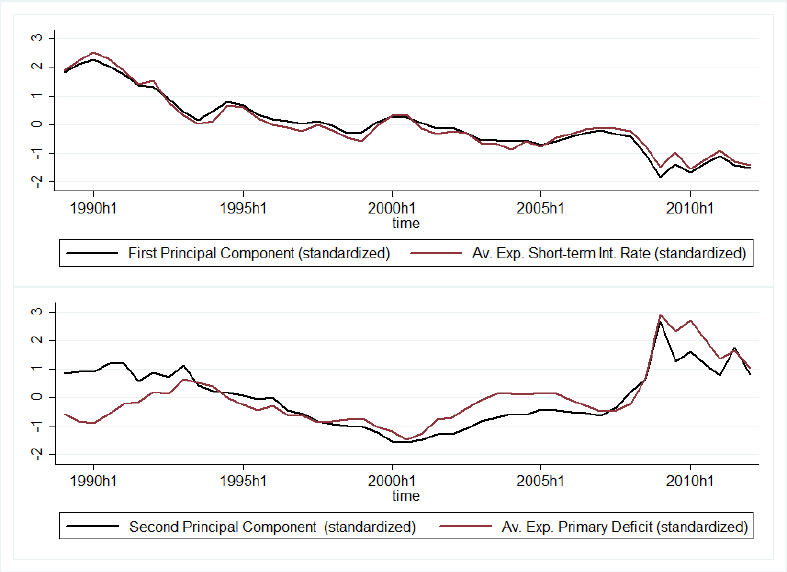
39
Figure 5. Global Factors and their Macroeconomic Interpretation
Note: The Figure shows the estimated unobserved factors plotted against their economic interpretation.
The top panel shows the first factor plotted against the average expected short-term interest rate of the
countries in the sample. The lower panel shows the second factor plotted against the average expected
deficit of the countries in the sample.
40
References
Alper, Emre C., Lorenzo Forni, 2011, “Public Debt in Advanced Economies and its Spillover
Effects on Long-Term Yields”, IMF Working Paper, No. 11/210 (Washington:
International Monetary Fund).
Afonso, Antonio, 2010, “Long-Term Government Bond Yields and Economic Forecasts:
Evidence for the EU” Applied Economics Letters, Taylor and Francis Journals, Vol.
17(15), pp. 1437–1441.
Ardagna, Silvia, and Francesco Caselli, and Timothy Lane, 2007, “Fiscal Discipline and the
Cost of Public Debt Service: Some Estimates for OECD Countries” The B.E. Journal
of Macroeconomics, Berkeley Electronic Press, Vol. 7(1).
Attinasi, Maria Grazia, and Cristina Checherita, and Christiane Nickel, 2009, “What Explains
the Surge in Euro Area Sovereign Spreads During the Financial Crisis of 2007–09?”,
ECB Working Paper Series, WP No 1131, December 2009.
Bai, Jushan, 2004, “Estimating Cross-Section Common Stochastic Trends in Nonstationary
Panel Data”, Journal of Econometrics, Elsevier, Vol. 122(1)
________, 2009, “Panel Data Models With Interactive Fixed Effects”, Econometrica,
Econometric Society, vol. 77(4), pp. 1229–1279, 07.
________, and Serena Ng, 2006, “Confidence Intervals for Diffusion Index Forecasts with a
Large Number of Predictors”, Econometrica, 74(4), pp. 1133–1150.
Baldacci, Emanuele and Sanjeev Gupta, and Amine Mati, 2008, “Is it (Still) Mostly Fiscal?
Determinants of Sovereign Spreads in Emerging Markets”, IMF Working Paper, No.
08/259 (Washington: International Monetary Fund).
________, and Manmohan, Kumar, 2010, “Fiscal Deficits, Public Debt and Sovereign Bond
Yields”, IMF Working Paper, No. 10/184 (Washington: International Monetary
Fund).
Barrios Salvador, and Per Iversen, and Magdalena Lewandowska and Ralph Setzer, 2009,
“Determinants of Intra-Ero Area Government Bond Spreads During the Financial
Crisis”, European Economy, Economic Papers 388.
Beber, Alessandro, Michael Brandt, and Kenneth Kavajecz, 2009, “Flight-to-Quality or
Flight-to-Liquidity? Evidence from the Euro-Area Bond Market”, Review of
Financial Studies, 22(3), pp. 925–957.
Beetsma, Roel and Massimo Giuliodori, 2010, “Fiscal Adjustment to Cyclical Developments
in the OECD: an Empirical Analysis Based on Real-Time Data”, Oxford Economic
Papers, Oxford University Press, vol. 62(3), pp. 419–441, July.
41
Bernoth, Kerstin, Jurgen Von Hagen, and Ludger Schuknecht, 2004, “Sovereign Risk Premia
in the European Government Bond Market,” Working Paper Series 369, European
Central Bank.
Buiter, Willem H., 2010, “The Limits to Fiscal Stimulus”, Oxford Review of Economic
Policy, Vol. 26, No 1, 2010, pp. 48–70.
Canzoneri, Matthew, and Robert Cumby, and Behzad Diba, 2002, “Should the European
Central Bank and the Federal Reserve be Concerned About Fiscal Policy?”,
Proceedings, Federal Reserve Bank of Kansas City, pp. 333–389.
Chinn, Menzie, and Jeffrey Frankel, 2007, “Debt and Interest Rates: The U.S. and the Euro
Area”, Economics Discussion Papers 2007-11, Kiel Institute for the World Economy.
________, and Hiro Ito, 2009, “A New Measure of Financial Openness”, Journal of
Comparative Policy Analysis, Volume 10, Issue 3 September 2008 , p. 309 - 322.
Chudik, Alexander, and Hashem Pesaran, and Elisa Tosetti, 2011, “Weak and Strong Cross-
Section Dependence and Estimation of Large Panels”, Econometrics Journal, Vol.
14, pp. C45–C90.
Ciarlone, Alessio, and Paolo Piselli, and Giorgio Trebeschi, 2009, “Emerging Markets”
Spreads and Global Financial Conditions”, International Financial Markets,
Institutions and Money, 19, pp. 222–239.
Cimadomo, Jacopo, 2008, “Fiscal Policy in Real Time”, ECB Working Paper Series, WP No.
919, 2008.
Claeys, Peter, and Moreno Rosina, and Jordi Suriñach, 2008, “Fiscal Policy and Interest
Rates: the Role of Financial and Economic Integration”, IREA Working Papers, 10,
University of Barcelona, Research Institute of Applied Economics.
Codogno, Lorenzo, and Carlo Favero, and Alessandro Missale, 2003, “Yield Spreads on
EMU Government Bonds”, Economic Policy, CEPR, CES, MSH, vol. 18(37), pp.
503–532, October.
Dell’Erba, Salvatore, and Sergio Sola, 2013,: “Fiscal Policy, Interest Rateds and Risk Premia
in Open Economy,” IHEID Working Papers 5-2013, Economics Section, The
Graduate Institute of International Studies.
Faini, Riccardo, 2006, “Fiscal Policy and Interest Rates in Europe”, Economic Policy, CEPR,
CES, MSH, vol. 21(47), pp. 443–489, 07.
42
Favero, Carlo, and Marco Pagano, and Ernst-Ludwig Von Thadden, 2009, “How Does
Liquidity Affect Bond Yields?”, Journal of Financial and Quantitative Analysis Vol.
45, No. 1, Feb. 2010, pp. 107.
Feldstein, Martin, 1986, “The Budget Deficit And The Dollar”, NBER Chapters, in: NBER
Macroeconomics Annual 1986, Volume 1, pp. 355–409 National Bureau of Economic
Research, Inc.
Forni, Mario, and Lucrezia Reichlin, 1998, “Let’s Get Real: A Factor Analytical Approach to
Disaggregated Business Cycle Dynamics”, Review of Economic Studies, 65, pp. 453–
473.
Gale, William, and Peter Orszag, 2002, “The Economic Effects of Long-Term Fiscal
Discipline”, Tax Policy Center Discussion Paper, December, Brookings Institutions.
________, and Peter Orszag, 2004, “Budget Deficits, National Savings, and Interest Rates”,
Brookings Papers on Economic Activity, (35)2004.
Geyer, Alois, Stephan Kossmeier and Stephan Pichler, 2004, “Measuring Systematic Risk in
EMU Government Yield Spreads”, Review of Finance, Vol. 8, pp. 171.
Giannone, Domenico, and Michele Lenza, 2008, “The Feldstein-Horioka Fact”, ECB
Working Paper Series, WP No. 873 (February).
________, and Michele Lenza, and Lucrezia Reichlin, 2009, Discussion of the paper “The
ECB and the Bond Market”, in Marco Buti, Servaas Deroose and Vito Gaspar editors,
The Euro, Cambridge University Press.
Giavazzi, Franceso, and Luigi Spaventa, 2010, “Why the Current Account Matters in a
Monetary Union: Lessons from the Financial Crisis in the Euro Area”, CEPR
Discussion Papers 8008, C.E.P.R. Discussion Papers.
Gomez-Puig, Marta, 2006, “Size Matters for Liquidity: Evidence from EMU Sovereign Yield
Spreads”, Economics Letters, Vol. 90(2), pp 156–162, February.
Gonzalez-Rozada, Martin and Eduardo Levy Yeiati, 2008, “Global Factors and Emerging
Market Spreads”, The Economic Journal, 118 (November), pp. 1917–1936.
Habib, Maurizio, and Livio Stracca, 2011, “Getting Beyond Carry Trade: What Makes a Safe
Haven Currency?”, ECB Working Paper Series, WP n. 1288, European Central Bank.
Laeven, Luc, and Fabian Valencia, 2008, “Systemic Banking Crises: A New Database”, IMF
Working Paper No. 08/224, (Washington: International Monetary Fund).
Laubach, Thomas, 2009, “New Evidence on the Interest Rate Effects of Budget Deficits and
Debt”, Journal of the European Economic Association, 7:4, pp. 858-885.
43
Manganelli, Simone and Guido Wolswijk, 2009, “Euro Bond Spreads”, Economic Policy,
Vol. 24, Issue 58, pp. 191-240, April 2009.
Mody, Ashoka, 2009, “From Bear Sterns to Anglo Irish: How Eurozone Sovereign Spreads
Related to Financial Sector Vulnerability”, IMF Working Paper, No. 09/108,
(Washington: International Monetary Fund).
Moon, Hyungsik R., and Benoit Perron, 2004, “Testing for a Unit Root in Panels with
Dynamic Factors”, Journal of Econometrics, Elsevier, vol. 122(1), pp. 81-126,
September.
Pesaran, Hashem, 2004, “General Diagnostic Tests for Cross Section Dependence in Panels”,
IZA Discussion Paper No. 1240.
________, 2006, “Estimation and Inference in Large Heterogenous Panels with Multifactor
Error Structure”, Econometrica, 74, 967-1012.
________, 2007, “A Simple Panel Unit Root Test in the Presence of Cross-Section
Dependence”, Journal of Applied Econometrics, John Wiley & Sons, Ltd., vol. 22(2),
pp. 265-312.
Poghosyan Tigran, 2012, “Long-run and Short-run Determinants of Sovereign Bond Yields
in Advanced Economies”, IMF Working Paper, No. 12/271 (Washington:
International Monetary Fund).
Reinhart, Vincent, and Brian Sack, 2000, “The Economic Consequences of Disappearing
Government Debt”, Brookings Papers on Economic Activity, Economic Studies
Program, The Brookings Institution, vol. 31, pp. 163- 220.
Sgherri, Silvia, and Edda Zoli, 2009, “Euro Area Sovereign Risk During the Crisis”, IMF
Working Paper No. 09/222, (Washington: International Monetary Fund).
Schuknecht, Ludger, and Jürgen von Hagen, and Guido Wolswijk, 2011, “Government Bond
Risk Premiums in the EU Rivisited: The Impact of the Financial Crisis”, European
Journal of Political Economy, Vol. 27, Issue 1, March 2011, pp. 36-43.
Thomas, Lloyd, and Danhua Wu, 2006, “Expected Future Budget Deficits and the U.S. Yield
Curve”, Business Economics, Palgrave Macmillan Journals, vol. 41(4), pp. 46-53,
October.
